Abstract
This paper introduces the concept of targeted field investigation on the reliability of earth-retaining structures in an active state, which is implemented in a random finite element method (RFEM) framework. The open source RFEM software REARTH2D was used and modified suitably in order to accommodate the purposes of the present research. Soil properties are modeled as random fields, and measurements are modeled by sampling from different points of the field domain. Failure is considered to have occurred when the “actual” resultant earth pressure force on the retaining wall (calculated using the friction angle random field) is greater than the respective “predicted” force (calculated using an homogenous friction angle field characterized by the mean of the values sampled from the respective random field). Two sampling strategies are investigated, namely, sampling from a single point and sampling from a domain, through an extensive parametric analysis. As shown, the statistical uncertainty related to soil properties may be significant and can only be minimized by performing targeted field investigation. Among the main findings is that the optimal sampling location in the active state is immediately adjacent to the wall face. In addition, it is advisable that the entire wall height be considered in sampling. Finally, it was observed that the benefit from a targeted field investigation is much greater as compared to the benefit gained using characteristic values in a Load and Resistance Factor Design framework.
1. Introduction
Uncertainties in soil properties arise from three main sources, namely, inherent variability, statistical uncertainty, and systematic uncertainties [1]. The inherent variability results from the fact that even in seemingly homogenous soil media, the soil properties exhibit variability by nature. Discrepancies between the laboratory and in situ conditions due to factors such as scale, anisotropy, and degree of saturation of soil are related to systematic uncertainties [1,2,3]. Statistical uncertainty (related to the mean and standard deviation of soil properties) is attributed to limited soil testing. Apparently, statistical uncertainty can be reduced by proper field investigation. Regarding the latter, it is mentioned that the current design codes are limited to some general recommendations (see Appendix A), focusing mainly on the extent of the subsurface exploration and aiming at identifying possible unfavorable geological conditions. In this respect, AASHTO [4] additionally recommends that samples be taken from locations alternating from in front of the wall to behind the wall. Apparently, this recommendation refers to structures such as sheet walls and pile walls, where undisturbed soil is retained and both active and passive states exist simultaneously. No recommendation is given for the sampling depth or distance from the wall.
The effect of soil sampling on the performance of geotechnical structures has been studied only by a few researchers. In this respect, Griffiths et al. [5] studied the effect of sampling on the reliability of passive earth pressure by using the random finite element method (RFEM). Considering a limited number of sampling locations (four in number), they concluded that a single sampling point located at horizontal distance equal to approximately one wall height from the wall results in a lower probability of failure independent of the spatial correlation length, and that the inclusion of additional sample points to characterize the soil properties reduces the probability of failure. Jaksa et al. [6] investigated the effect of soil variability and site investigation scope on the footing’s settlement of a three-story building and observed that the likelihood of under-designing or over-designing a footing decreases as the scope of the investigation increases. Yang et al. [7] used conditional random fields enabling the site investigation data to be incorporated directly in probabilistic analysis, and they found that the coefficient of variation of factor of safety can be reduced by incorporating more site investigation data. Ching and Phoon [8] addressed the statistical uncertainties associated with the estimation of a depth-dependent trend function and spatial variation about the trend function using limited site-specific geotechnical data. This study proposed a two-step approach to characterize the uncertainties in all parameters, including the functional form of the trend, within a consistent Bayesian framework. Yang et al. [9] studied the importance of sampling location on slope stability assessment based on statistical hypothesis testing, concluding that the slope crest is the optimal location to conduct geotechnical site exploration. Fenton et al. [10] studied the effect of the number of samples and type of trend removal on residual uncertainty. They found that removing the sample mean outperforms removing the best linear unbiased estimate (BLUE) when the actual field correlation length is small, but the BLUE is better to use if the actual correlation length is large relative to the domain size. In addition, they found that more samples reduce the uncertainty when the field correlation length is small but do not have much impact when the field correlation length is large. Li et al. [11] linked 3D conditional random fields with finite elements, within a Monte Carlo framework, to investigate optimum sampling locations and the cost-effective design of a slope. Their results clearly demonstrate the potential of 3D conditional simulation in directing exploration programs and designing cost-saving structures.
The present paper investigates numerically the effect of targeted field investigation on the reliability of earth-retaining structures. This involves sampling from a specific point or a set of points (i.e., adopting a sampling strategy) so that the statistical uncertainty in the design is minimized (the probability of failure is minimized). The specific sampling is called optimal. This study is based on the random finite element method (RFEM) [5], properly considering soil sampling in the analysis. The RFEM method combines elasto-plastic finite element analysis with the random field theory. The random fields are generated using the local average subdivision method [12] and mapped onto the finite element mesh, taking full account of element size in the local averaging process. Each random field is fully described by its mean, standard deviation, and spatial correlation length. The latter is defined as the distance within which the soil property shows relatively strong correlation or persistence from point to point [13].
Contrary to the common belief that statistical uncertainty decreases with an increasing number of samples [14,15,16,17], the present analysis will show that the statistical error in an active earth pressure analysis can be minimized only by targeted field investigation. Apparently, this study refers to structures such as sheet pile and bored pile walls retaining undisturbed soil and not to backfilled retaining structures.
2. Brief Description of the RFEM Program Used
The open source RFEM program REARTH2D (http://www.engmath.dal.ca/rfem; see also Fenton and Griffiths [18] and Griffiths et al. [5]) is used and modified suitably in order to accommodate the purposes of the present research. The program involves the generation and mapping of soil properties (cohesion, friction angle, and/or unit weight; at least one of these parameters is required to be random) onto a finite element mesh. For a specific set of material random fields, the program returns the wall reaction force and overturning moment caused by the self-weight of a spatially random soil. In addition, from the same set of random fields, the REARTH2D program is able to sample soil property values for calculating the respective wall reaction force and overturning moment based on Rankine’s [19] earth pressure theory, considering that the soil medium is homogenous and characterized by the sampled values (mean of the values sampled for each soil property). The procedure is repeated times; is the number of realizations, where each realization refers to a new set of random fields for , , and . Then, the failure probability of the wall against sliding or overturning is calculated. The “failure probability” is defined by the fraction of the number of realizations that result in a specific type of failure (sliding or overturning) over the total number of realizations. In each RFEM realization, “failure” is considered to have occurred when the “actual” wall reaction force (or overturning moment) referring to the spatially random soil (value calculated using the RFEM method) is greater than the respective (factored or unfactored) predicted value referring to soil having spatially uniform properties sampled from the RFEM random fields (value calculated based on Rankine’s earth pressure theory as mentioned above). That is, it stands that
where the symbol denotes either wall reaction force or overturning moment ( and respectively), the subscript denotes active state of failure, and is the user-defined safety factor. In the REARTH2D program, the active state is reached incrementally. However, in practice, retaining structures do not always work under large wall movements; thus, the active state may not be fully reached. Ni et al. highlighted the importance of the intermediate active (or passive) state in design [20]. Reducing the increments in the finite element analysis and thus not allowing the active state to be fully reached, the authors observed, as expected, greater wall reaction forces but no change in the optimal sampling location. Thus, avoiding any confusion, the analysis that follows refers to fully reached active states.
Favoring objectivity in the comparison between the “actual” and the respective “predicted” values, the original REARTH2D program has been modified by the authors so as to calculate the wall reaction force and overturning moment based on the finite element method instead of Rankine’s theory. That is, the failure probability is defined as follows:
The finite-element earth pressure analysis in REARTH2D uses an elastic, perfectly plastic Mohr–Coulomb constitutive model with stress redistribution achieved iteratively using an elasto-viscoplastic algorithm essentially similar to that described in the text by Smith and Griffiths [21]. The boundary conditions on the right side of the mesh (across the wall) are such that they allow vertical but not horizontal movement, while the base of the mesh is fully restrained. The top and left sides of the mesh are unrestrained, except for the nodes adjacent to the ‘wall’, which are as described immediately below.
The active state against sliding is modeled by translating the nodes of the mesh next to the wall horizontally and uniformly away from the soil. These nodes have fixed horizontal components of displacement. As active conditions are mobilized, the vertical components of these displaced nodes are either free to move down or restrained depending on whether a perfectly smooth or perfectly rough wall is modeled. Considering a rough, rigid wall, the active state against rotation is modeled by imposing the same angular displacement to the nodes next to the wall, having as a pivot point the lower point of wall; in this respect, the (cross-sectional) width of the wall is considered to be infinitesimally small. For smooth rotating walls, these nodes are allowed to slip downwards along the wall surface. The translation or rotation of the wall is performed incrementally. The finite element analysis is terminated when the incremental displacements have resulted in the active reaction force reaching its minimum limiting value.
3. Parametric Study for Determining the Optimal Sampling Strategy
This paper examines the case of a wall retaining a fully drained cohesionless soil against active failure in plane strain conditions. Different sampling strategies are examined, i.e., sampling from a single point and sampling from a domain, through a parametric analysis for defining the strategy that minimizes the probability of failure and thus the statistical error (i.e., the optimal sampling strategy).
The soil mass is discretised into a 48 × 34 mesh (number of elements at the horizontal and vertical direction respectively) consisting of eight-noded square elements with side lengths equal to 0.1 (Figure 1). Various wall heights are considered ranging from H = 1.4 m to 2.9 m (meaning that the wall extends to a depth ranging from 14 to 29 elements), while the mesh geometry has been kept the same for all cases. A 24-element wall will be generally considered in the analysis (hereafter called a “reference wall”); the other wall heights will be used for the investigation of the effect of wall height on the optimal sampling strategy. The 48-element mesh in the horizontal direction was chosen so that the failure mechanism in the RFEM analysis will not be affected by the proximity of the right boundary. In this respect, for the highest wall considered (29-element-high wall), as the value approaches zero (extreme case), according to Rankine’s theory, the failure mechanism in the active state will occupy a horizontal distance from the wall face equal to one wall height (that is, 29 elements; value 40% smaller as compared to the 48 horizontal elements of the geometry).
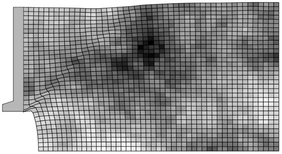
Figure 1.
Active earth failure of the “reference” wall. Graphical representation of a random field of (this is a typical random finite element method (RFEM) realization); light areas correspond to lower friction angles and vice versa. For the soil shown, and = 0.3.
In this study, both and are treated as log-normal random fields. The soil is assumed cohesionless with = 30° and = 20 kN/m3, while various standard deviation and values are examined. Moreover, since depends on (the initial horizontal stresses are defined by Jaky’s [22] equation), this is also treated as a random field. In addition, it is mentioned that although the elastic parameters of soil (ν and E) affect the required wall movement in order for the active state to be fully reached, preliminary parametric analysis carried out by the authors showed that they have no influence on the optimal sampling strategy. Thus, these values have been kept constant and equal to 0.3 and 105 kN/m2 respectively throughout the entire analysis presented herein. Furthermore, the random fields are assumed to have the same spatial correlation length and an exponentially decaying (Markovian) correlation structure (see [18]):
Finally, a safety factor FS equal to 1.3 is generally assumed in the analysis; the effect of FS on the sampling strategy is also investigated later.
As samples are taken from a material field (i.e., the ground), which simultaneously is a stress field (stresses caused by the self-weight of the soil and also any external load), the location of the optimal sampling points is affected by the coexistence of these two fields. Aiming at finding the optimal sampling strategy, the following parameters will be examined: the sampling depth and horizontal distance () for the case of sampling from a single point (measured from the soil surface and the wall face, respectively), the sampling domain length and horizontal distance () of the continuous probing test location for the case of sampling from a domain (measured as in the previous case), the spatial correlation length of soil , the wall roughness (perfectly smooth or perfectly rough wall), the wall height , the coefficient of variation () of and , the mean value of , and the safety factor value considered and the soil mass anisotropy . Hereafter, it is noted that the symbol (that is, without subscript) denotes isotropic conditions . Four sampling scenarios are indicatively shown in Figure 2 (scenarios A and B refer to a single sampling point, whilst scenarios C and D refer to continuous probing tests).
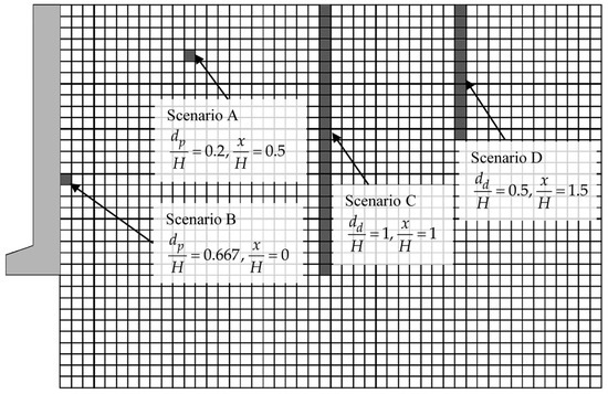
Figure 2.
Graphical representation of different sampling scenarios: Scenarios A and B refer to a single sampling point (each located at depth dp), whilst Scenarios C and D refer to sampling domains (each having length dd).
The optimal sampling point or domain will be identified by comparing the failure probability values derived by various sampling strategies. Apparently, when dealing with small differences in values, the stability of the results is very important. In this respect, the number of realizations was set equal to 3000; this number, as discussed in Appendix B, can be considered adequate for the needs of the present research. The effect of the element size is also examined in the same appendix.
3.1. Sampling from a Single Point
3.1.1. Effect of Spatial Correlation Length
Example charts showing the variation of with respect to for various values are given in Figure 3. From this figure, it is inferred that the optimal sampling location for the active case is clearly for zero horizontal distance from the wall, both for the case of translating and rotating wall and for any value. Isolating the curves for = 0 (see Figure 4), it seems that there is a “worst case spatial correlation length”—see also [23], where the failure probability becomes maximum. For example, for the various ratios shown in Figure 4 (ranging from = 0.04 to 8.3), the = 0.21 case gives the higher values. From Figure 4, it is also inferred that as tends to zero, the value tends to a single value for any depth (that is, is independent of the sampling depth). However, as increases, the value becomes more dependent on the sampling depth.
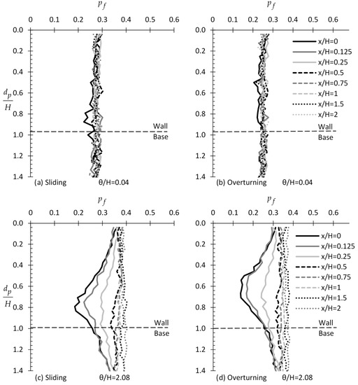
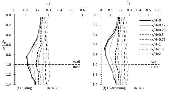
Figure 3.
versus example curves for various and values for the case of sliding (figure (a,c,e)) and overturning wall (figure (b,d,f)).
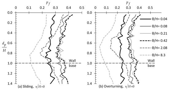
Figure 4.
versus example curves for various values and (smooth wall) for the case of (a) sliding and (b) overturning wall.
3.1.2. Effect of Wall Roughness
The effect of wall roughness on the location of the optimal sampling point is examined herein. The optimal sampling distance was also found to be at = 0; therefore, results are presented only for this case (see Figure 5). Comparing Figure 4 with Figure 5 (for a perfectly smooth and a perfectly rough wall, respectively), it is inferred that the statistical error is generally less sensitive to the sampling depth in the case of a rough wall. However, comparing similar soil–wall systems but with different wall roughness, it can be said that by choosing the proper sampling depth, smaller values can be obtained when the wall is smooth.
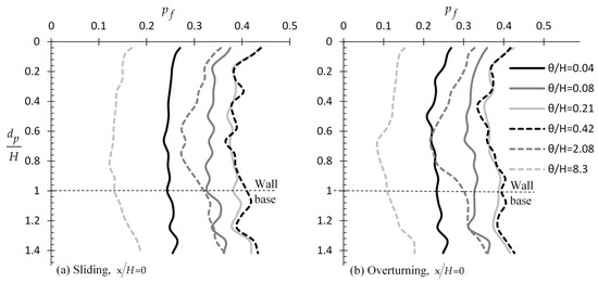
Figure 5.
versus example curves for various values and (perfectly rough wall) for the case of (a) sliding and (b) overturning wall; please compare with Figure 4 (perfectly smooth wall).
3.1.3. Effect of Wall Height
The variation of with for various wall height values, i.e., = 1.4, 1.9, 2.4, 2.9 m, is shown in Figure 6. From this figure, it is clear that the wall height has a minor influence on the location of the optimal sampling point.
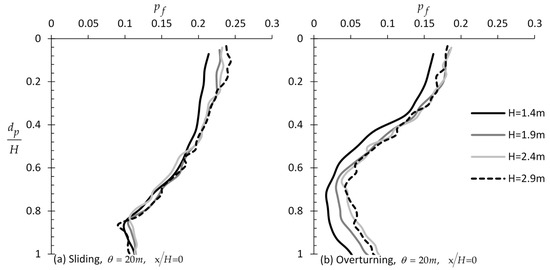
Figure 6.
versus example curves for different wall heights, H, and = 20 m for the case of (a) sliding and (b) overturning wall.
3.1.4. Effect of COV of and
In this paragraph, six values for and were considered, i.e., = 0.0, 0.1, 0.2, 0.3, 0.4, and 0.5. The optimal sampling distance from the wall was found not to be affected by the of and , where again the = 0 case leads to the smaller statistical error. Thus, only the = 0 case will be presented here. From Figure 7, it is generally inferred that the of and has no effect or a minor effect on the optimal sampling depth for the sliding and rotating case, respectively.
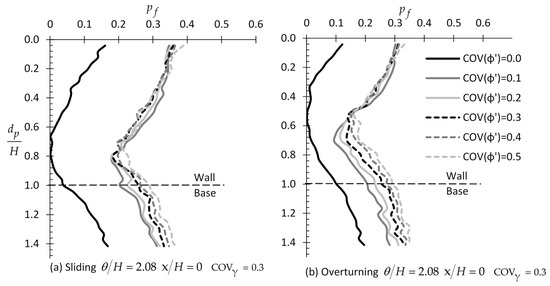
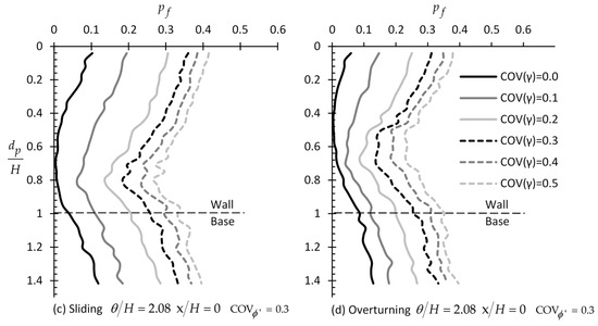
Figure 7.
versus example relationships by considering different values of COV of and γ; figure (a,b) refer to COV of , whilst figure (c,d) refer to COV of γ for the sliding and overturning moments, respectively.
3.1.5. Effect of and
So far, the mean value of was equal to 30° in all cases considered in the analysis. The influence of on the optimal sampling location is examined herein. In this respect, three values were considered, i.e., = 20°, 30°, and 40°. The of was set equal to 0.3, while the of was set to zero. The authors found that the optimal sampling distance was again at = 0 for any value (not shown here for space economy). In addition, from Figure 8, it is inferred that the of soil has no effect on the optimal sampling depth both in the case of translating and rotating wall. The same stands for .
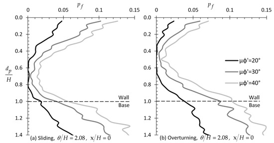
Figure 8.
versus example relationships for (a) sliding and (b) overturning wall considering different values.
3.1.6. Effect of the Factor of Safety
The variation of with respect to for different values is shown in Figure 9; the optimal sampling distance from the wall face was also found to be at = 0 for any value. Thus, only the = 0 case is presented here. From Figure 9, it is obvious that the failure probability decreases as increases, but what is not trivial is that the positive effect of targeted field investigation on the reduction of the statistical error is greater for greater values. For example, considering the case of the rotating wall, as shown in Figure 9, the value when = 1.1 is approximately 0.45 and independent of the ratio. For the same soil–wall system, if = 1.5, ranges from 0.18 for = 0 (and 1.4) to almost zero for = 0.6.
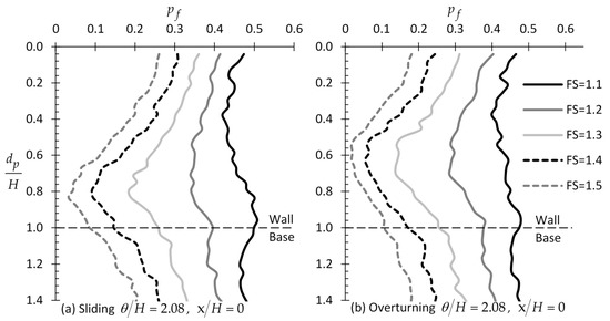
Figure 9.
versus example curves for different values for the case of (a) sliding and (b) overturning wall.
3.1.7. Effect of Soil Anisotropy
According to the literature, the spatial variability of soil in the horizontal direction is much greater than the respective one in the vertical direction due to natural deposition and soil formation processes. In this respect, these studies mention that the horizontal spatial correlation length is generally about 10 times the vertical one . For example, for Vanmarcke [24], for Soulie et al. [25] and Cherubini [26], for Popescu et al. [27], for Phoon and Kulhawy [28], and ≈ 2 to 7 times the value for Firouzianbandpey et al. [29].
Driven from these findings, the effect of soil anisotropy on the optimal sampling location will be investigated here by comparing the case with the case. The reference wall–soil system with = = 2.08 will be compared with a respective one having = 2.08 and = 20.8. The variation of with for various values is shown in Figure 10. From this figure, it is inferred that the statistical error practically remains the same for horizontal sampling distances less than one wall height for both the translating and rotating wall cases. Although for the difference in the values is very small, again, the optimal sampling location is at . Comparing Figure 10a with Figure 3c and Figure 10b with Figure 3d, it can be said that the effect of the horizontal sampling location is significantly higher in the isotropic case. Regarding the optimal sampling location, the soil anisotropy has no effect on the optimal sampling depth both in the case of the translating and rotating wall.
3.2. Sampling from a Domain
This sampling strategy refers to data referring to continuous probing tests (e.g., the Cone Penetration Test or Standard Penetration Test). The length of the sampling domain is always measured from the soil surface, whilst arithmetic mean values are used for the various soil properties in the Finite Element Method (FEM) analysis (see Section 2).
Since each (finite) element (see Figure 1) has edge 0.1 length units (in this respect, meters), sampling is considered to take place every 0.1 m (along the vertical direction). The minimum and maximum sampling domain length considered were 0.1 m (rather referring to a single point) and 3.4 m, respectively. It is noted that for all cases examined in this section, the optimal sampling distance was found again to be at = 0. Thus, for space economy, the analysis below generally refers to the = 0 case.
3.2.1. Effect of Spatial Correlation Length
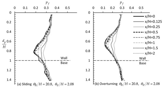
Example charts showing the variation of with respect to for various and values are given in Figure 11, both for the case of sliding and rotation of the wall; it is reminded that was set equal to 1.3 (recall Equation (2)). From this figure, it is inferred that the optimal horizontal sampling distance from the wall is again for = 0, although for very small theta values, the horizontal sampling distance makes no noticeable difference. However, as the theta value increases, the role of horizontal distance becomes more significant. Given now that soil samples will be taken from = 0, it is advisable, as it is inferred from Figure 11, that the entire domain length along the wall is considered, especially for the rotational mode of failure. This practice may significantly reduce the statistical error. It is also interesting that, extending the sampling domain beyond the maximum depth of wall (i.e., > 1), the statistical error remains constant. Finally, from Figure 11, it is inferred that a “worst case theta” exists. This is more obvious in Figure 12, showing the variation of with for various values and = 0.
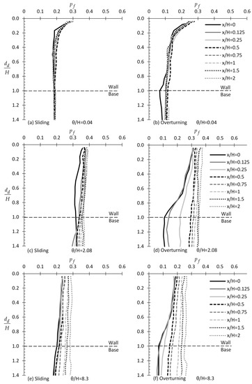
Figure 11.
versus example relationships for different values of scaled correlation length and lateral distance from the wall face (). Figure (a,c,e) refer to the case of sliding wall whilst figure (b,d,f) to the case of overturning wall.
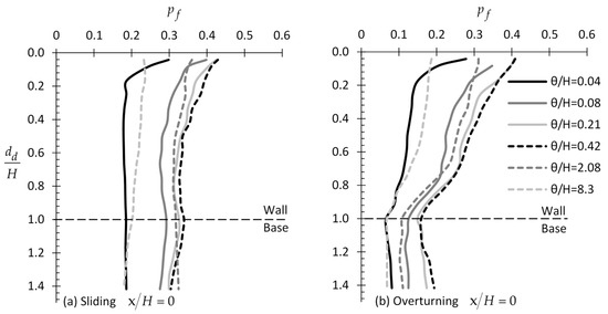
Figure 12.
versus example relationships for the case of (a) sliding and (b) overturning wall by considering different scaled values.
3.2.2. Effect of Wall Roughness
Generally, the wall roughness has a minor effect on the optimal sampling domain length, although, as expected (see Figure 13), it noticeably affects the failure probability. As shown in Figure 13, a great reduction in the statistical error can be achieved only in the case of a smooth rotating wall, with the optimal sampling domain length being the entire wall height. Characteristically, it is mentioned that the minimum failure probability is obtained for = 1 and that this probability remains constant for greater values.
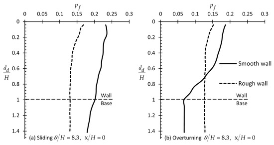
Figure 13.
versus example curves for = 8.3 and (rough and smooth wall) for the case of (a) sliding and (b) overturning wall.
3.2.3. Effect of Wall Height
In this paragraph, four wall heights were considered, i.e., = 1.4, 1.9, 2.4, and 2.9 m. Figure 14 presents the variation of with for these four cases. From this figure, it is clear that the wall height has only a minor influence on the sampling domain length (see also Section 3.1.3).
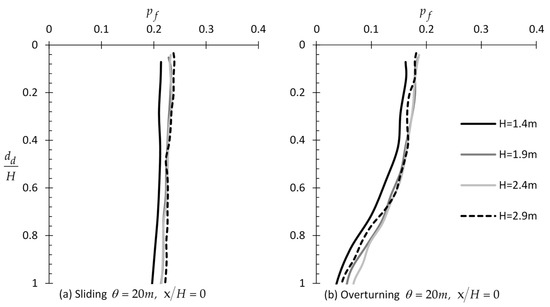
Figure 14.
versus example curves for different wall heights and for the case of (a) sliding and (b) overturning wall.
3.2.4. Effect of COV of and
In this paragraph, six values for and were considered, i.e., = 0.0, 0.1, 0.2, 0.3, 0.4, and 0.5. The optimal horizontal sampling distance from the wall was found not to be affected by the of or , where again the = 0 case leads to the smaller probabilities of failure. Thus, only the = 0 case will be presented here. From Figure 15, it is generally inferred that the of and has no or a minor effect on the optimal sampling length for the sliding and rotating case, respectively.
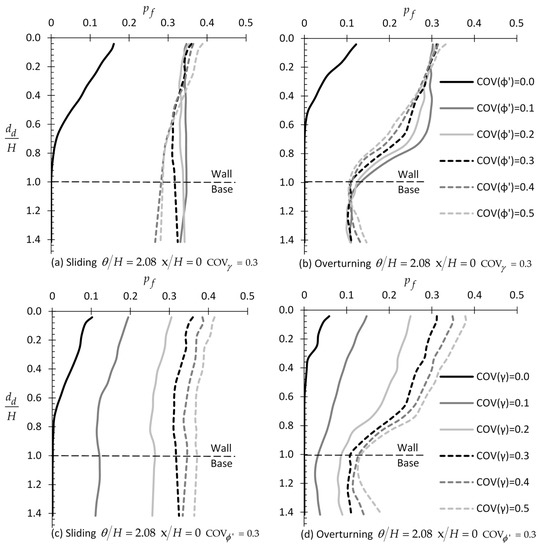
Figure 15.
versus example relationships by considering different values of COV of (figure (a,b)) and γ (figure (c,d)); figure (a,c) refer to the case of sliding wall, whilst figure (b,d) refer to the case of overturning wall.
3.2.5. Effect of the Factor of Safety
The variation of with respect to for different values is shown in Figure 16; the optimal sampling distance was also found to be at = 0 for any value. Thus, only this case is presented here. From Figure 16, it is obvious that the failure probability decreases as increases, but what it is not trivial is that the positive effect of targeted field investigation on (that is, decrease in ) is greater for greater values.
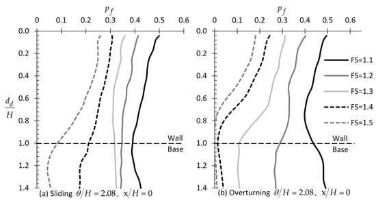
Figure 16.
versus example curves for different values for the case of (a) sliding and (b) overturning wall.
3.2.6. Effect of Soil Anisotropy
In this paragraph, the retaining soil is considered to be highly anisotropic having = 20.8 and = 2.08; for the isotropic case, it stands that = = = 2.08. The optimal horizontal sampling distance from the wall was found not to be affected by the anisotropy of soil, where again the = 0 case leads to the smallest probabilities of failure; thus, only the = 0 case is presented here. From Figure 17, it is generally inferred that the soil anisotropy has also no effect on the sampling domain length for sliding or rotating cases.
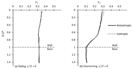
Figure 17.
versus example curves for the case of (a) sliding and (b) overturning wall considering anisotropic soil ( and ) and isotropic soil ().
4. Discussion
4.1. Optimal Sampling Locations
One of the main outcomes derived from the present analysis is that the optimal horizontal sampling location in the active state of stress is at = 0, that is, immediately adjacent to the wall face. This came as a surprise, as someone would expect the optimal location to lie on or in the close vicinity of Rankine’s 45° + /2 failure plane passing through the lower point of the wall. Actually, based on authors’ findings [30], this is the case for the passive state. Regarding Rankine’s earth pressure theory, it is reminded that there is not a single failure plane, but rather an infinite number of such planes, parallel to the one mentioned above encompassing all of the others [31]. A common characteristic of these planes is that their lower point is in contact with the wall. In this respect, it seems that the optimal sampling location in the active case shows preference to this array of points. Regarding now the depth of the optimal sampling point, it was found that this lies at a depth greater than the 2/3 or 1/2 of the wall height for the sliding and rotational mode of failure respectively; the exact depth depends on the spatial correlation length of the soil. For the optimal sampling domain length, it is advisable that the entire wall height be considered.
4.2. The Importance of Targeted Field Investigation in Practice
The importance of targeted field investigation, where samples are taken from a priory known optimal locations, is highlighted here. For a random material field referring to a specific RFEM realization (such as the one presented in Figure 1), it can be said that it convincingly represents a real field. For the three examples presented in this paragraph, the reference wall (and the finite element mesh) of Figure 1 will be used, whilst the material properties are given in Table 1. These materials differ from each other, in essence, in the spatial correlation length and only for the first material; in addition to the friction angle of the soil, the unit weight is a random field. Besides, as it is inferred from the present research, the mean and values of and have no effect on the optimal sampling location. The random field of used in each example is shown in Figure 1, Figure 18 and Figure 19, respectively. It is reminded that the light areas correspond to lower friction angles and vice versa. The FS value is assumed unity (recall Equation (2)); this factor is discussed in the next paragraph.

Table 1.
Summary of the characteristics of the soils used in the three examples (wall height H = 2.4 m).
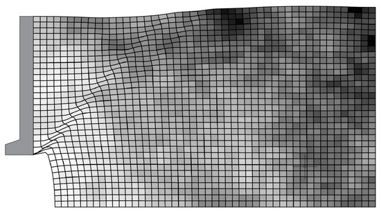
Figure 18.
Graphical representation of the random field of of Example #2 ( = 4.2; see Table 1). Light areas correspond to lower friction angles and vice versa.
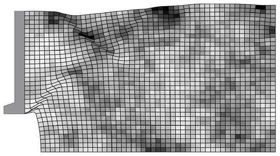
Figure 19.
Graphical representation of the random field of of Example #3 ( = 0.42; see Table 1). Light areas correspond to lower friction angles and vice versa.
The predicted resultant driving force (F) or moment (M) acting on the wall is compared against the respective “actual” ones. For each one of the examples presented herein, the latter derives from the respective random field of using the RFEM method (in Example #1, in addition to , γ is also a random field). The predicted F and M values derive from a homogenous soil field characterized by the mean of the values sampled from the original (random) field. The results are presented in Figure 20, Figure 21 and Figure 22 in Fpredicted/F“actual” or Mpredicted/M“actual” versus x/H form for various /H values. The relative difference Rd is also given in each chart (secondary vertical axis; a positive value indicates design on the safe side and vice versa; Rd is equal to Fpredicted/F“actual”-1 or Mpredicted/M“actual”-1 for the case of forces and moments respectively).
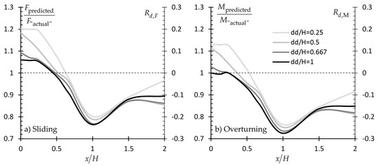
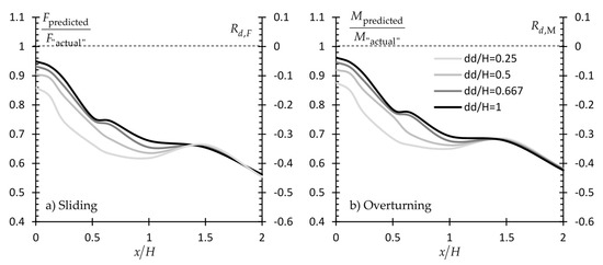
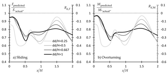
If the suggestions related to the horizontal distance from the wall and the domain length (x/H = 0 and dd/H = 1 respectively) are valid, the Fpredicted/F“actual” and Mpredicted/M“actual” ratios for this specific sampling scenario should logically be equal to unity or very close to this value. The readers should bear in their mind that a Fpredicted/F“actual” or Mpredicted/M“actual” value close to unity or equal to unity for a x/H value other than zero does not indicate that this x/H location is an optimal sampling location. As the soil retained by the wall is a spatially random field, a set of samples taken from points away from the wall face may also give (coincidentally) a mean value equal (or approximately equal) to the respective one obtained from a set of samples taken from the x/H = 0 location.
As shown in Figure 20, Figure 21 and Figure 22, the Fpredicted/F“actual” and Mpredicted/M“actual” ratio values for x/H = 0 are very close to unity or equal to unity, indicating the validity of authors’ suggestions. Indicatively, it is mentioned that the abrupt drop of the Fpredicted/F“actual” (or Mpredicted/M“actual”) versus x/H curves in Figure 20 between x/H = 0.5 and 1.5 is attributed to the “dark” (strong) area appearing at this particular location, as shown in Figure 1. From Figure 20, Figure 21 and Figure 22, it is also confirmed that a vertical sampling domain of length equal to the wall height gives better prediction for the destabilizing forces acting on the wall.
A comparison between the figures given in Section 3 with the respective ones given in Section 4 shows clearly that statistical uncertainty does not necessarily decrease with the increasing number of samples. Indeed, the opposite may easily happen. For example, comparing the pf ≈ 0.03 value for x/H = 0 shown in Figure 3f (single point case) with the pf ≈ 0.26 value for x/H = 2 (case of 24 sampling points) shown in Figure 11f, it is obvious that statistical uncertainty can only be minimized by targeted field investigation. Such examples can also be found in the present section; please compare the case of {x/H = 2, dd/H = 1} with the {x/H = 0, dd/H = 0.25} in Figure 21b giving Rd,M ≈ −0.42 and −0.12, respectively.
4.3. Designing with Load and Resistance Factor Design (LRFD) Codes
Recent geotechnical design codes (such as Eurocode 7 [32] and AASHTO [4]) aim to achieve geotechnical designs with an appropriate target reliability by applying partial factors to characteristic parameter values. In principle, the characteristic values of geotechnical parameters are selected so as to take account of the inherent variability of the ground, the uncertainty in the determination of the soil parameters and the extent of the relevant failure mechanism. “Partial factors” are also applied to actions, material properties, and/or resistances to provide safety and also to account for model uncertainties and dimensional variations [33]. Meanwhile, Eurocode 7 [32] defines the characteristic value of a geotechnical parameter as “a cautious estimate of … the mean of a range of values covering a large surface or volume of the ground”. In the various codes of North America, the mean value of the measurements is used [4,34,35,36]. Eurocode 7 further notes that “if statistical methods are used, the characteristic values should be derived such that the calculate probability of a worse value governing the occurrence of the limit state under consideration is not greater than 5%”. In this respect, the following statistical equation is often used for the calculation of the characteristic value [33,37]:
where is the sample mean, is the sample standard deviation, is the number of samples, is the Student factor for a confidence level of α% in the case of degrees of freedom, and is equal to , assuming a normal distribution. values for a confidence level of 95% and various degrees of freedom in tabular form can be found in any statistical book (e.g., [38]).EN 1997-1 [32] dictates that the design values of the geotechnical parameters be derived from the respective characteristic values using the following equation:
where is the characteristic value of a material property and the symbol denotes the partial material factor. When partial factors are not applied to the material properties (i.e., = 1), a model factor greater than 1 is applied to the resistances.
The discussion on the design of earth-retaining structures based on characteristic soil property values instead of the respective mean values is facilitated by the two example charts in Figure 23. These charts refer to Case #3 presented in the previous paragraph (see also Table 1). This specific case was chosen because of the relatively low θ value (i.e., θ/H = 0.42), which indicates a rather highly spatially variable soil; thus, the use of the characteristic value makes more sense. Two cases are presented, the dd/H = 1 and the dd/H = 0.25. The figure in question refers to the sliding mode of failure; however, the respective curves for the overturning mode of failure do not differ appreciably. It is also mentioned that, in the example presented here, the partial material factor for the friction angle = was set equal to unity.
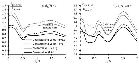
Figure 23.
Fpredicted/F“actual” vs. x/H curves using both mean and characteristic values (dashed and solid lines respectively) for FS = 1 and 1.3. Figure referring to the case of a sliding wall and to two sampling domain cases (dd/H = 1 (figure (a)) and to dd/H = 0.25 (figure (b))). The reference wall was used. Soil characteristics as shown in Table 1 (Example #3).
From Figure 23, it is clear that the benefit from a targeted field investigation is much greater as compared to the benefit gained using characteristic values. Moreover, despite the conservatism which is inserted in the analysis using the characteristic value concept, the characteristic values alone, as shown, cannot guaranty a conservative enough engineering study. The safety level can be increased by applying a statistical uncertainty partial factor (similar to the model factor γR used by Eurocode 7) or a unified and more conservative model factor to the resistances, which will absorb the statistical uncertainties related to the soil. In this respect, a partial factor equal to 1.3 has also been applied (FS = 1.3; recall Equation (2)) in the present example. As shown in Figure 23, the use of such a factor simply displaces upwards (that is, to the safe side) the Fpredicted/F“actual” (or Mpredicted/M“actual”) versus x/H curves. The inclusion of the “characteristic value” in the REARTH2D code has been done by the authors.
5. Conclusions
The present research clearly shows that statistical uncertainty related to soil properties may be significant and that it can only be minimized by performing targeted field investigation; the latter is defined by the number and location of sampling points. As samples are taken from a material field (i.e., the ground), which simultaneously is a stress field (stresses caused by the self-weight of the soil and any external load), the location of the optimal sampling points is affected by the coexistence of these two fields. Two main sampling strategies were investigated—namely, sampling from a single point and sampling from a domain—through an extensive parametric analysis.
One of the main findings of the present analysis is that the optimal horizontal sampling location in the active state is at = 0—that is, immediately adjacent to the wall face. Regarding the depth of the optimal sampling point, it was found that this lies at depth greater than two-thirds or one-half of the wall height for the sliding and rotational mode of failure respectively; the exact depth depends on the spatial correlation length of the soil. For the optimal sampling domain length, it is advisable that the entire wall height be considered.
In addition, it was observed that the benefit from a targeted field investigation is much greater as compared to the benefit gained using characteristic soil property values. Moreover, despite the conservatism which is inserted in the analysis using the characteristic value concept, the characteristic values alone, as shown, cannot guaranty a conservative enough engineering study. The safety level can be increased by applying a statistical uncertainty partial factor (similar to the model factor γR used by Eurocode 7) or a unified and more conservative model factor to the resistances, which will absorb the statistical uncertainties related to the soil.
Author Contributions
Conceptualization, L.P. and P.C; methodology, P.C. and L.P.; software, P.C.; validation, E.G.; formal analysis, P.C.; writing—original draft preparation, P.C.; writing—review and editing, P.C., L.P. and E.G.; visualization, P.C.; supervision, L.P. and E.G.
Funding
This research was funded by the Cyprus University of Technology, grant number EX-20081.
Conflicts of Interest
The authors declare no conflict of interest.
Notation List
| drained cohesion | |
| COV | coefficient of variation of a soil parameter e.g., COV() and COV() for drained friction angle and unit weight of soil respectively. |
| sampling domain length measured always from the uppermost point of the wall | |
| depth of sampling point | |
| modulus of elasticity of soil | |
| safety factor | |
| resultant wall reaction force | |
| excavation depth | |
| wall height | |
| coefficient of earth pressure at rest | |
| resultant wall reaction moment | |
| number of realizations | |
| number of samples | |
| probability of failure | |
| sample standard deviation | |
| embedded length of the support | |
| Student t factor for a confidence level of α% in the case of degrees of freedom | |
| horizontal distance from wall face | |
| design values of geotechnical parameters | |
| characteristic value | |
| sample mean | |
| investigation depth below the ground level | |
| unit weight of soil | |
| partial factor for the friction of soil | |
| partial material factor | |
| model factor | |
| spatial correlation length (also, it replaces the symbols and when = ) | |
| horizontal spatial correlation length | |
| vertical spatial correlation length | |
| mean unit weight of soil | |
| mean of drained friction angle | |
| Poisson’s ratio of soil | |
| Lag distance or separation distance between two measurements | |
| drained friction angle |
Appendix A. Subsurface Exploration by Various Design Codes
Subsurface explorations shall provide the information needed for the design and construction of structures. However, in this respect, the current design codes are limited to some general recommendations, not indicating specific sampling locations that may effectively reduce statistical uncertainty.
For example, for excavations in normal geological conditions protected by retaining structures, EN 1997-2:2007 [39] recommends that where the piezometric surface and the groundwater tables are below the excavation base, the investigation depth, , be greater than or equal to and where the piezometric surface and the groundwater tables are below the excavation base, , the recommendation is that it be greater than or equal to ; if no stratum of low permeability is encountered down to these depths, then .
In turn, AASHTO [4] recommends a minimum of one exploration point per retaining wall; for retaining walls more than 30 m in length, investigation points spaced every 30 to 60 m with locations alternating from in front of the wall to behind the wall are recommended. For the minimum depth of exploration, AASHTO suggests that the investigation be extended at least to a depth below the bottom of the wall where the stress increases due to the estimated foundation load being less than 10% of the existing effective overburden stress at the depth and between 1 and 2 times the wall height.
Appendix B. Stability of Numerical Results (Number of Realizations Considered in the RFEM Models) and Effect of Element Size
As shown in Figure A1, 3000 realizations can be deemed sufficient for the problem studied herein. Although the versus number of realizations curves of the figure in question refer to = 0.667 and (when not mentioned) to , the same results are taken for other sampling locations.
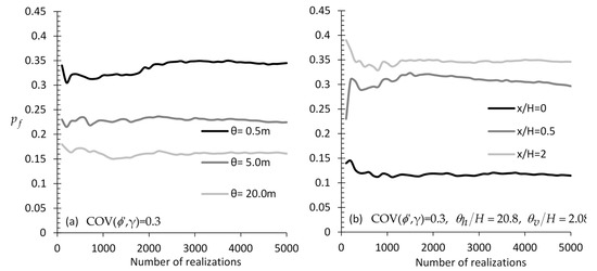
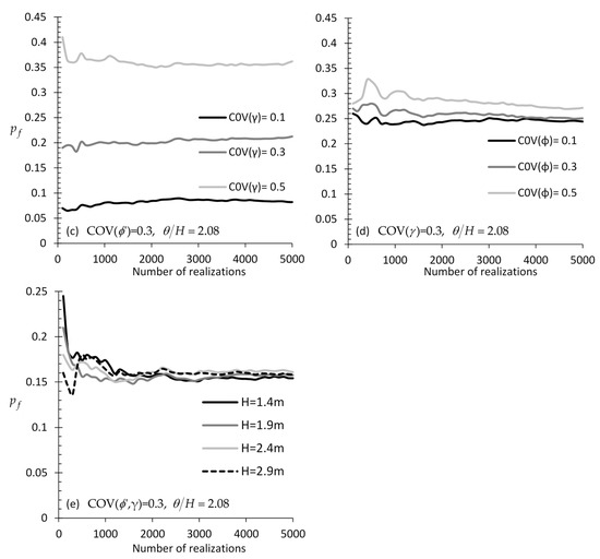
Figure A1.
versus number of realizations charts for different (a) correlation length values (case of isotropic field), (b) values (case of anisotropic field), (c) COV value of (isotropic field), (d) COV value of (isotropic field), and (e) wall heights; figures referring to sampling from and .
Regarding the element size, it is recommended that this be less than the half of the spatial correlation length, although an element size equal to the does not introduce great error in the analysis (e.g., see the comparison chart of Figure A2 where the reference wall has been used).
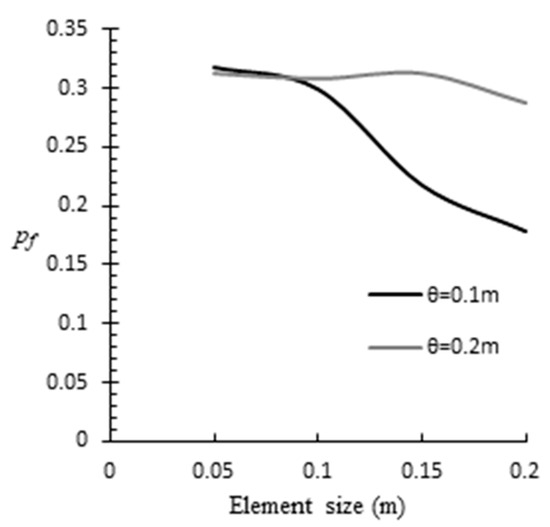
Figure A2.
Effect of element size on the failure probability.
References
- Duzgun, H.S.B.; Yucemen, M.S.; Karpuz, C. A probabilistic model for the assessment of uncertainties in the shear strength of rock discontinuities. Int. J. Rock Mech. Min. Sci. 2002, 39, 743–754. [Google Scholar] [CrossRef]
- Tang, W.H.; Zhang, L. Quality assurance and risk reduction in foundation engineering. In Frontier Technologies for Infrastructures Engineering: Structures and Infrastructures Book Series; Chen, S.-S., Ang, A.H.-S., Eds.; CRC Press: Boca Raton, FL, USA, 2009; Volume 4, pp. 123–142. [Google Scholar]
- Christian, J.T.; Ladd, C.C.; Baecher, G.B. Reliability applied to slope stability analysis. J. Geotech. Eng. 1994, 120, 2180–2207. [Google Scholar] [CrossRef]
- AASHTO. AASHTO LRFD Bridge Design Specifications; American Association of State Highway and Transportation Officials: Washington, DC, USA, 2010; ISBN 9781560514510. [Google Scholar]
- Griffiths, D.V.; Fenton, G.A.; Ziemann, H.R. Reliability of passive earth pressure. Georisk 2008, 2, 113–121. [Google Scholar] [CrossRef]
- Jaksa, M.B.; Goldsworthy, J.S.; Fenton, G.A.; Kaggwa, W.S.; Griffiths, D.V.; Kuo, Y.L.; Poulos, H.G. Towards reliable and effective site investigations. Géotechnique 2005, 55, 109–121. [Google Scholar] [CrossRef]
- Yang, R.; Huang, J.; Griffiths, D.V.; Sheng, D. Probabilistic Stability Analysis of Slopes by Conditional Random Fields. Geo-Risk 2017 2017, 450–459. [Google Scholar]
- Ching, J.; Phoon, K.-K. Characterizing uncertain site-specific trend function by sparse Bayesian learning. J. Eng. Mech. 2017, 143, 4017028. [Google Scholar] [CrossRef]
- Yang, R.; Huang, J.; Griffiths, D.V.; Li, J.; Sheng, D. Importance of soil property sampling location in slope stability assessment. Can. Geotech. J. 2019, 56, 335–346. [Google Scholar] [CrossRef]
- Fenton, G.A.; Naghibi, F.; Hicks, M.A. Effect of sampling plan and trend removal on residual uncertainty. Georisk Assess. Manag. Risk Eng. Syst. Geohazards 2018, 12, 253–264. [Google Scholar] [CrossRef]
- Li, Y.J.J.; Hicks, M.A.A.; Vardon, P.J.J. Uncertainty reduction and sampling efficiency in slope designs using 3D conditional random fields. Comput. Geotech. 2016, 79, 159–172. [Google Scholar] [CrossRef]
- Fenton, G.A.; Vanmarcke, E.H. Simulation of random fields via local average subdivision. J. Eng. Mech. 1990, 116, 1733–1749. [Google Scholar] [CrossRef]
- Vanmarcke, E.H. Probabilistic modeling of soil profiles. J. Geotech. Eng. Div. 1977, 103, 1227–1246. [Google Scholar]
- Orr, T.L.L. Managing risk and achieving reliable geotechnical designs using Eurocode 7. In Risk and Reliability in Geotechnical Engineering; Phoon, K.K., Ching, J., Eds.; CRC Press: Boca Raton, FL, USA, 2014; pp. 395–433. [Google Scholar]
- Ching, J.; Phoon, K.-K. Constructing multivariate distributions for soil parameters. Risk Reliab. Geotech. Eng. 2015, 3–76. [Google Scholar]
- Huang, X.C.; Zhou, X.P.; Ma, W.; Niu, Y.W.; Wang, Y.T. Two-dimensional stability assessment of rock slopes based on random field. Int. J. Geomech. 2016, 17, 4016155. [Google Scholar] [CrossRef]
- Imanzadeh, S.; Denis, A.; Marache, A. Settlement uncertainty analysis for continuous spread footing on elastic soil. Geotech. Geol. Eng. 2015, 33, 105–122. [Google Scholar] [CrossRef]
- Fenton, G.; Griffiths, D.V. Risk Assessment in Geotechnical Engineering; Wiley: Hoboken, NJ, USA, 2008; ISBN 9780470178201. [Google Scholar]
- Rankine, W.J.M., II. On the stability of loose earth. Philos. Trans. R. Soc. London 1857, 9–27. [Google Scholar]
- Ni, P.; Mangalathu, S.; Song, L.; Mei, G.; Zhao, Y. Displacement-dependent lateral earth pressure models. J. Eng. Mech. 2018, 144, 4018032. [Google Scholar] [CrossRef]
- Smith, I.M.; Griffiths, D.V. Programming the Finite Element Method, 4th ed.; Wiley: Hoboken, NJ, USA, 2004; ISBN 0470011246. [Google Scholar]
- Jaky, J. The coefficient of earth pressure at rest. J. Soc. Hungarian Archit. Eng. 1944, 355–388. [Google Scholar]
- Griffiths, D.V.; Zhu, D.; Huang, J.; Fenton, G.A. Observations on probabilistic slope stability analysis. In Proceedings of the 6th Asian-Pacific Symposium on Structural Reliability and Its Applications (APSSRA 2016); Huang, J.L., Zhang, J., Chen, J., Eds.; Tongji University: Shanghai, China, 2016. [Google Scholar]
- Vanmarcke, E.H. Reliability of earth slopes. J. Geotech. Eng. Div. 1977, 103, 1247–1265. [Google Scholar]
- Soulie, M.; Montes, P.; Silvestri, V. Modelling spatial variability of soil parameters. Can. Geotech. J. 1990, 27, 617–630. [Google Scholar] [CrossRef]
- Cherubini, C. Data and considerations on the variability of geotechnical properties of soils. In Proceedings of the International Conference on Safety and Reliability, ESREL, Lisbon, Portugal, 17–20 June 1997; Volume 97, pp. 1583–1591. [Google Scholar]
- Popescu, R.; Prévost, J.H.; Deodatis, G. Effects of spatial variability on soil liquefaction: Some design recommendations. Geotechnique 1997, 47, 1019–1036. [Google Scholar] [CrossRef]
- Phoon, K.; Kulhawy, F. Characterization of geotechnical variability. Can. Geotech. J. 1999, 36, 612–624. [Google Scholar] [CrossRef]
- Firouzianbandpey, S.; Griffiths, D.V.; Ibsen, L.B.; Andersen, L.V. Spatial correlation length of normalized cone data in sand: Case study in the north of Denmark. Can. Geotech. J. 2014, 51, 844–857. [Google Scholar] [CrossRef]
- Christodoulou, P.; Pantelidis, L.; Gravanis, E. The effect of targeted field investigation on the reliability of earth retaining structures in passive state. 2019; manuscript in preparation. [Google Scholar]
- Venkatramaiah, C. Geotechnical Engineering; Revised 3r.; New Age International: New Delhi, India, 2006; ISBN 812240829X. [Google Scholar]
- EN 1997-1. Eurocode 7 Geotechnical Design—Part 1: General Rules; CEN (European Committee for Standardization): Brussels, Belgium, 2004. [Google Scholar]
- Orr, T.L.L. Defining and selecting characteristic values of geotechnical parameters for designs to Eurocode 7. Georisk Assess. Manag. Risk Eng. Syst. Geohazards 2016, 11, 103–115. [Google Scholar] [CrossRef]
- Canadian Standards Association. Canadian Highway Bridge Design Code. CAN/CSA-S6-14; Canadian Standards Association: Mississauga, ON, Canada, 2014. [Google Scholar]
- Phoon, K.K.; Kulhawy, F.H.; Grigoriu, M.D. Development of a Reliability-Based Design Framework for Transmission Line Structure Foundations. J. Geotech. Geoenviron. Eng. 2003, 129, 798–806. [Google Scholar] [CrossRef]
- Fenton, G.A.; Naghibi, F.; Dundas, D.; Bathurst, R.J.; Griffiths, D.V. Reliability-based geotechnical design in 2014 Canadian Highway Bridge Design Code. Can. Geotech. J. 2015, 53, 236–251. [Google Scholar] [CrossRef]
- JGS. Principles for Foundation Design Grounded on a Performance-Based Design Concept (GeoGuide); Japanese Geotechnical Society: Tokyo, Japan, 2004. [Google Scholar]
- White, J.; Yeats, A.; Skipworth, G. Tables for Statisticians, 3rd ed.; Nelson Thornes: Cheltenham, UK, 1979; ISBN 085950462X. [Google Scholar]
- EN 1997-2. Eurocode 7-Geotechnical Design-Part 2: Ground Investigation and Testing; CEN (European Committee for Standardization): Brussels, Belgium, 2007. [Google Scholar]
© 2019 by the authors. Licensee MDPI, Basel, Switzerland. This article is an open access article distributed under the terms and conditions of the Creative Commons Attribution (CC BY) license (http://creativecommons.org/licenses/by/4.0/).