Article

Temperature Analysis of Obstacle Lighting Lamp Working under Various Ambient Conditions: Theoretical and Practical Experiments

1
Faculty of Electrical Engineering Automatic Control and Informatics, Opole University of Technology, Prószkowska 76, 45-758 Opole, Poland
2
BSSTC.PL Sp. z o.o., Technologiczna 2A, 45-839 Opole, Poland
*
Author to whom correspondence should be addressed.
Appl. Sci. 2019, 9(22), 4951; https://doi.org/10.3390/app9224951
Submission received: 1 October 2019 / Revised: 4 November 2019 / Accepted: 14 November 2019 / Published: 17 November 2019
(This article belongs to the Section Applied Industrial Technologies)

Abstract

:

Featured Application

Featured Application: The results of the experimental tests were carried out in the laboratory of BSSTC.PL Sp. z o.o. and OLATECH DR INZ. Andrzej Błachowicz using an obstacle lighting lamp that is currently in production. The developed simulation model, which has been verified experimentally, was used to determine the influence of changes in meteorological parameters on the temperature distributions on the surface of the lamp. It will be used in the future to optimize the geometry of the heat sink used in the lamp in terms of electricity consumption and thermal resistance. It is planned to extend the application of the lamp under difficult climatic conditions.

Abstract

The article presents the results of experimental and theoretical works aimed at determining the distribution of heat emitted by an obstacle lighting lamp. These kind of lamps are commonly applied as a warning for air traffic vehicles. There is a need for lighting devices with various intensities, whose application depends on the location and operating conditions. The overall aim of the author’s work is to develop a computer model that would enable us to conduct research aimed at determining the optimal parameters of lamp operation without the need to build many physical models. Measurements of heat emitted by a currently manufactured lamp were made, and based on these, a numerical model of the lamp operating under laboratory conditions was developed. The considered lamp has two heat sources, one of which is light-emitting diodes (LEDs), while the other heat source consists of stabilizers and other elements of the lamp power supply system. After positive experimental verification of the numerical model, theoretical analyses of heat emission under various meteorological conditions were carried out, while the values of ambient temperature and airflow velocity were changed; then, the influence of these parameters on the temperature distribution on the surface of the lamp was determined.

1. Introduction

The subject matter of the article is related to obstacle lighting lamps working in air traffic safety systems. Nowadays, such lamps are a crucial part of the warning system for air traffic vehicles due to the expansion of the world’s aerial navigation [1]. They are also subject to international standards and air traffic rules, as established by the International Civil Aviation Organization [2], which are applied worldwide by the National Civil Aviation of various countries. Particular technological parameters as colors, luminous intensity, patterns, and also the location of the warning lamp installation are defined by these standards. These kind of lamps are commonly attached to tall structures such as e.g., chimneys, towers, transmission lines, or wind power turbines to make them visible for air traffic vehicles, especially in the night. There exist lighting devices of various intensities on the market, whose application depends on the location and operating conditions, e.g., under high pollution or mist environment. Depending on the particular location, it may be a hot or cold climate; thus, there exists a need for the lamps to operate under different weather and environmental conditions.
Nowadays, it is a frequent procedure in the industry to perform computer simulations for complex systems instead of building numerous physical models of a device, which leads to savings in time and money [3]. For example, the subject of optimizing the size and shape of heat sinks for various lighting devices is now widely researched, especially in the field of numerical modeling, e.g., [4]. Frequently discussed in the literature is the cooling of light-emitting diode (LED) lamps with the use of natural and forced convection, e.g., [5,6,7]. Current trends in heat sink optimization in various constellations are described in detail in [8]. There are also published works of numerical analysis of the LED modules [9], but in our case, the whole model of the lamp is crucial. In [10], the authors consider a comparable subject matter, and a similar heating curve for a street lamp has been obtained, but their numerical model does not refer to the transient state but only to the steady state. Often, the published papers concern only theoretical analyses, without referring to a physical model, e.g., [7,11]. A lot of interesting information about the modeling and measuring of LED-based light sources can be found in [12].
The main goal of the authors is to develop a device with the ability to work in extremely difficult weather conditions. For example, the lamps currently being produced by BSSTC.PL Sp. z o.o. and OLATECH DR INZ. Andrzej Błachowicz are sold on the European market, but it is planned to develop a device that is able to operate in desert and equatorial conditions. An appropriate device, which is continuously illuminated, prior to its application in the industry needs to satisfy requirements according to national/international standards. Therefore, a computer model that enabled conducting research aimed at determining the optimal parameters of the lamp operation was developed. In particular, a simplified numerical model of the device was built using COMSOL Multiphysics and its Heat Transfer module, which applies the finite element method (FEM) for the calculation of integrated physics of heat propagation and airflow under the laminar regime. The model was validated using experimental data in a steady state. In subsequent sections, the numerical model, the measurement, and theoretical investigations results are presented.

2. Materials and Methods

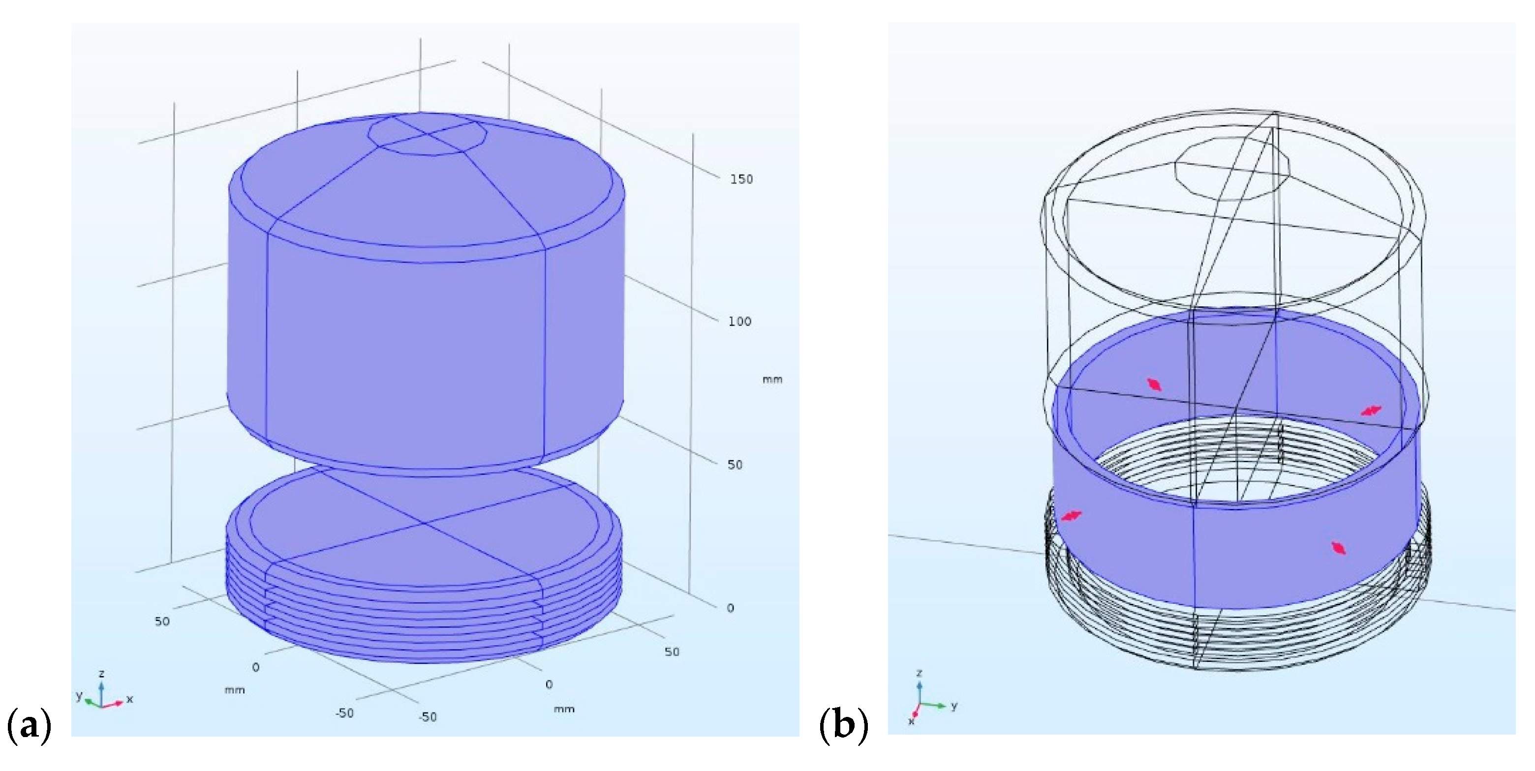
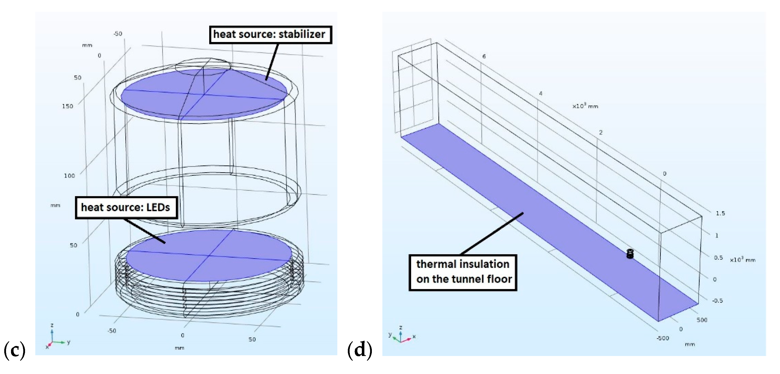
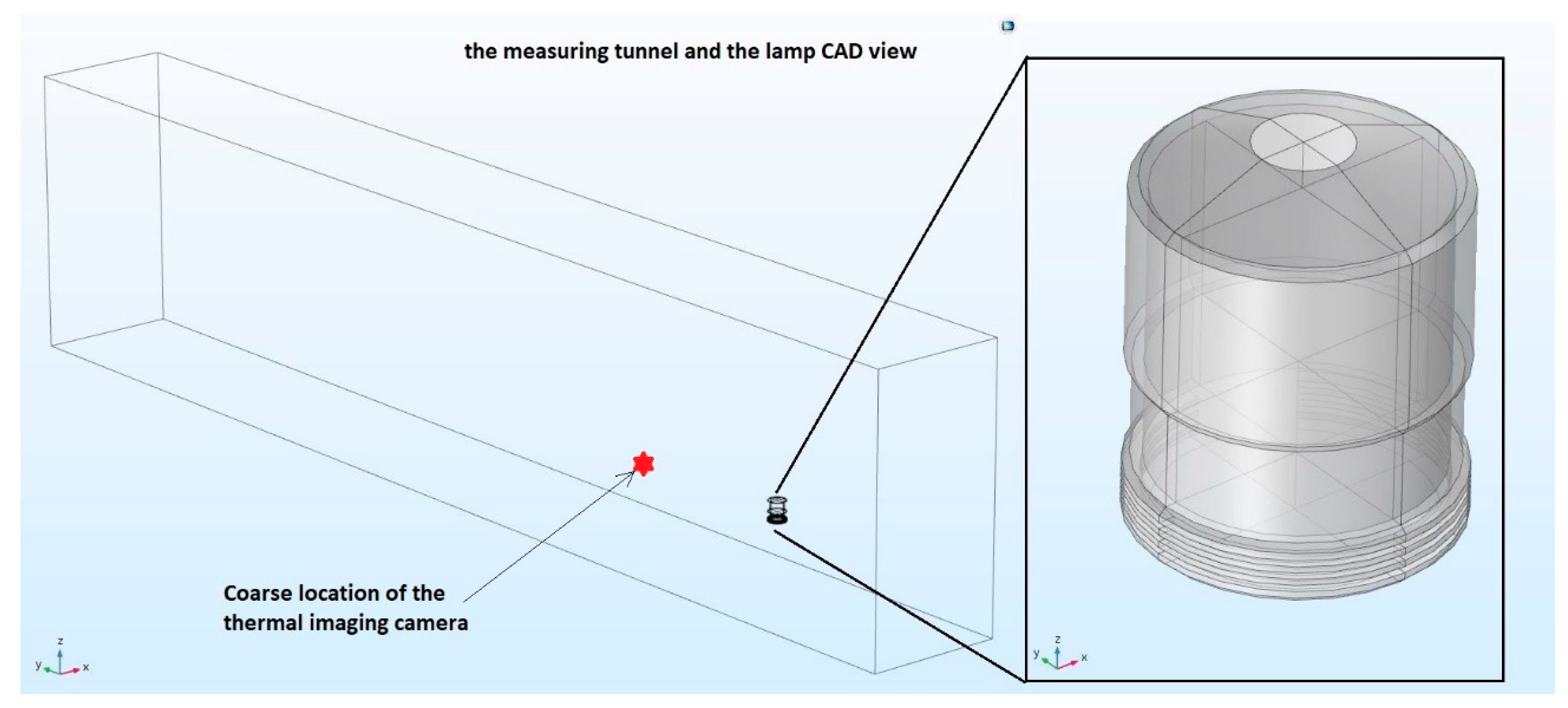
2.1. The Object under Study

The article considers experimental and theoretical works aimed at determining the distribution of heat emitted by an obstacle lighting lamp. The object under study has two heat sources, one of which is LEDs emitting light, and the other consists of stabilizers and other elements of the lamp power supply system. For the purpose of experimental tasks, the lamp was installed in the front part of a rectangular tunnel made of chipboard, with dimensions W × H × L = (1 × 2 × 8.8) m. For the measurement of heat emitted by the lamp, a thermal imaging camera type VIGOcam v5 from VIGO System S.A. was applied. This device is equipped with a bolometric matrix of a resolution 384 × 288 px, where pixel size equals 25 × 25 µm; the registered spectral range is 8–14 µm. The applied lens has a diameter of 35 mm with a spatial resolution of 0.7 × 10⁻³ rad. The emissivity was corrected to value relevant for red paint and equals 0.96. The camera was located in the tunnel at 1.75 m distance from the lamp at its hight, using a tripod rack. The measurement conditions were controlled in such a manner that the tunnel was closed, no forced airflow was present, and the ambient temperature was stable at 28 °C.
For the purpose of theoretical analysis, a simplified model of the lamp and the tunnel was implemented. The CAD (computer-aided design) drawing of the computational domain depicting the rectangular tunnel with the lamp and an enlarged view of the lamps is depicted in Figure 1, where also the coarse location of the thermal imaging camera is marked.
The lamp has a cylindrical shape of a maximal radius equal to 54.47 mm. The simplified numerical model of the lamp consists of two heat sinks made of aluminum covered with paint (see Figure 2a) and a transparent, light-transmittable cylinder made of acrylic plastic (plexiglass) of 5 mm width (see Figure 2b). The LEDs emitting light are installed on a printed circuit board at the surface of the bottom heat sink, while the stabilizers and other elements of the power supply system are mounted inside the top heat sink. The theoretical model assumes that the heat produced by the LEDs and stabilizers is evenly distributed over the area directly adjacent to the heat sink; therefore, we define a surface heat source for the LEDs and stabilizer, as depicted in Figure 2c. For the outer edge of the computational domain, we assume a constant ambient temperature, while the tunnel floor is assumed to be thermally insulated (see Figure 2d).
In the first step, measurements of the heat emitted by the lamp in the tunnel were registered from the moment the lamp was switched on until the temperature was stabilized, which under laboratory conditions lasted about 7 h. Based on the gathered results, the numerical model was verified in order to adjust all the model parameters, which are described in the next section. After the experimental verification process, theoretical analyses of heat emission under various meteorological conditions were carried out. Simulations in both the transient and stationary state were performed, while the value of ambient temperature and airflow velocity were changed; then, the influence of these parameters on the temperature distribution on the surface of the lamp was determined.
For theoretical calculations, we applied a PC computer featuring an Intel(R) Xeon(R) CPU E5-1650 v4 @ 3.60GHz with 12 cores. For the computational problem, which was connected with solving large linear equation systems resulting from discretized partial differential equations, as described in Section 2.3, we applied an efficient Geometric Multigrid Solver [13], which applies hierarchical algorithms. Furthermore, the PARDISO package was applied, which improves the efficiency and performance, especially on shared-memory multiprocessor systems [14,15].

2.2. Governing Equations and Model Parameters

The governing equation for heat transfer calculation in the transient state is given by Equation (1). For steady-state calculations, the terms with time and time derivatives are omitted.
ρ C p T t + ρ C p u · T + · q = Q + Q p + Q vd + Q ted ,
q = k T ,
where T is the dependent variable for temperature (K), t is time (s), ρ is the density (kg/m3), Cp is the specific heat capacity at constant stress (J/(kg·K)), q is the heat flux (W/m2), u is the velocity vector (m/s), k is thermal conductivity (W/m·K), Q contains other heat sources (W/m3), Q vd   =   τ : u is heat sources for viscous dissipation in fluid (W/m3), Q p = α T p t + u · p is total point heat sources resulting in pressure work (W/m3), Q ted = α T : d S d t is thermoelastic dumping in solids (W/m3), τ is viscous stress tensor (Pa), p is pressure (Pa), S is the second Piola–Kirchhoff stress tensor (Pa), and α = 1 ρ ρ T is the coefficient of thermal expansion (1/K).
The thermal insulation boundary condition for the tunnel floor (see Figure 2d) is defined by Equation (3), while the other tunnel boundaries are subject to changes defined by the ambient temperature, as defined in Equation (4).
n · q = 0 ,
T = T a m b ,
The theoretical model involves diffuse surface equations for the transparent part made of acrylic plastic, which are given by Equations (5)–(9). Equations defined for the aluminum surface are given by Equations (10) and (11).
n · q = ε u ( G u n 2 σ T 0 4 ) + ε d ( G d n 2 σ T 0 4 ) ,
( 1 ε u ) G u = j u ε u n 2 σ T 0 4 ,
( 1 ε d ) G d = j d ε d n 2 σ T 0 4 ,
G u = G m , u ( j ) + F amb , u n 2 σ T amb , u 4 + G extDir , u + G extDiff
G d = G m , d ( j ) + F amb , d n 2 σ T amb , d 4 + G extDir , d + G extDiff  
n · q = ε ( G m ( j ) + F amb n 2 σ T amb 4 + G extDir + G extDiff n 2 σ T 0 4 ) ,
( 1 ε ) ( G m ( j ) + F amb n 2 σ T amb 4 + G extDir + G extDiff ) = j ε n 2 σ T 0 4 ,
where T 0 is the external temperature (K), n is the normal vector (-), ε u ,   ε d represent the upside and downside for the surface emissivity for acrylic plastic, ε u   =   ε d   = 0.15 , ε is the surface emissivity for aluminum (covered with red paint), ε = 0.96 , n 2 σ T 4 corresponds to blackbody emissive power according to Stefan–Boltzmann law (W/m2), n is the refractive index for the media (1), σ is the Stefan–Boltzmann constant (W/m2·K4), j is surface radiosity (W/m2), ju, jd is surface radiosity upside and downside, Famb is ambient view factor, in which Famb,u, Famb,d are respectively the upside and downside, Gm is mutual surface irradiation (W/m2), in which Gm,u and Gm,d are respectively the upside and downside, GextDir represents the directional external irradiation sources (W/m2), in which GextDir,u, GextDir,d are respectively the upside, and downside, Tamb is the ambient temperature (K), of which Tamb,u, Tamb,d are respectively the upside and downside, GextDiff represesnts the diffuse external irradiation sources (W/m2).
The assumed model parameters are summarized in Table 1. The other parameter values assumed in the numerical model are as follows: the heat source simulating the heat emitted due to the operation of LEDs was defined as the heat rate equal to QLED = 29 W/m2, the heat source simulating the heat emitted due to the operation of stabilizers was defined as the heat rate equal to QSTAB = 23 W/m2, the ambient temperature Tamb was varied in the range from 24 to 44 °C, but for the verification process Tamb = 28 °C, the x-axis velocity component vx of the velocity vector u was varied in the range from 0 to 10 m/s, while the other components were assumed zero, except for the verification process vx = 0 m/s. The inner part of the lamp and the tunnel was filled with air.

2.3. Discretization Mesh

As mentioned above, the FEM method was applied for the calculations. In this method, the object under study is divided into a finite number of elements with the preset size of Δx, which results in a so-called mesh. The application of this method enables approximating the temperature values in each element of the mesh using a function described with a number of parameters, which is called degrees of freedom (DoF). For each mesh element xj, two terms are defined—DoFj = p(xj) and φj(x)—which for the whole computational domain results in a set of functions p(x) as expressed by Equation (12).
p ( x ) = j D o F j ϕ j ( x ) ,
The DoFj elements constitute the calculation result. The number of finite elements within the calculation domain is dependent on the particular element size. In the considered model, three different areas, with varied values, were defined for the tunnel (T), for the lamp (L), and for the lamp vicinity (V), as summarized in Table 2. Selected grid sizes result from the optimization of the duration of calculations while maintaining a high accuracy of the results. The area close to the lamp, where significant temperature changes take place, has been compacted with grid elements, while remote areas have been divided into a smaller number of elements. For the whole computational domain, the resulting mesh settings are defined in Table 3.

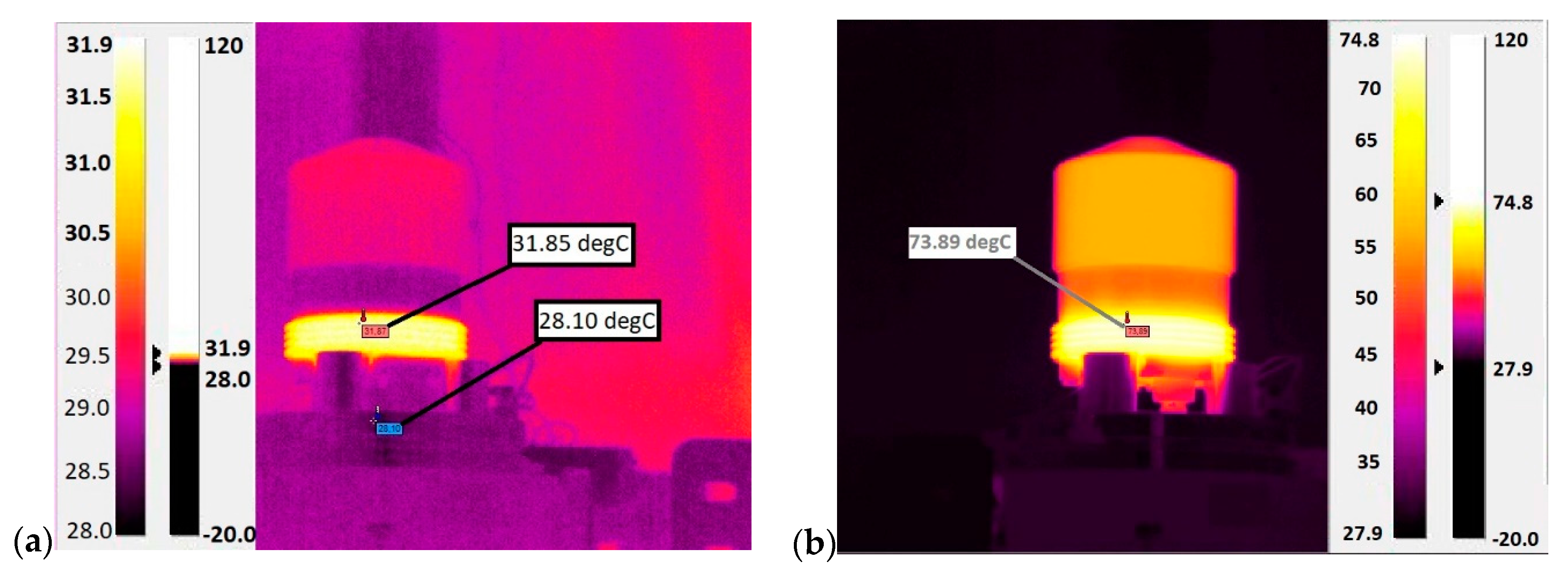
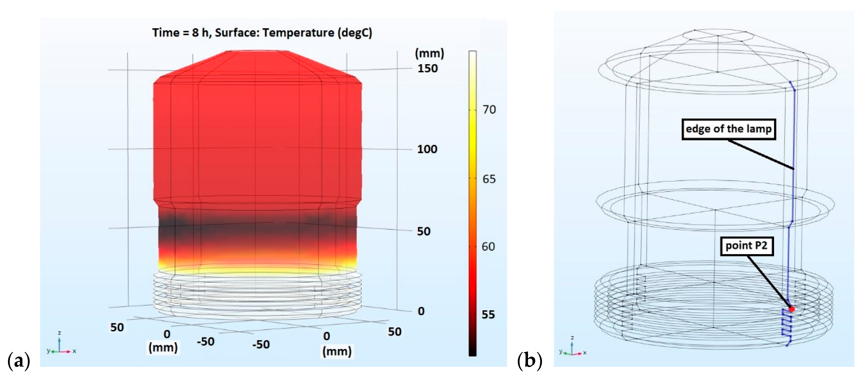
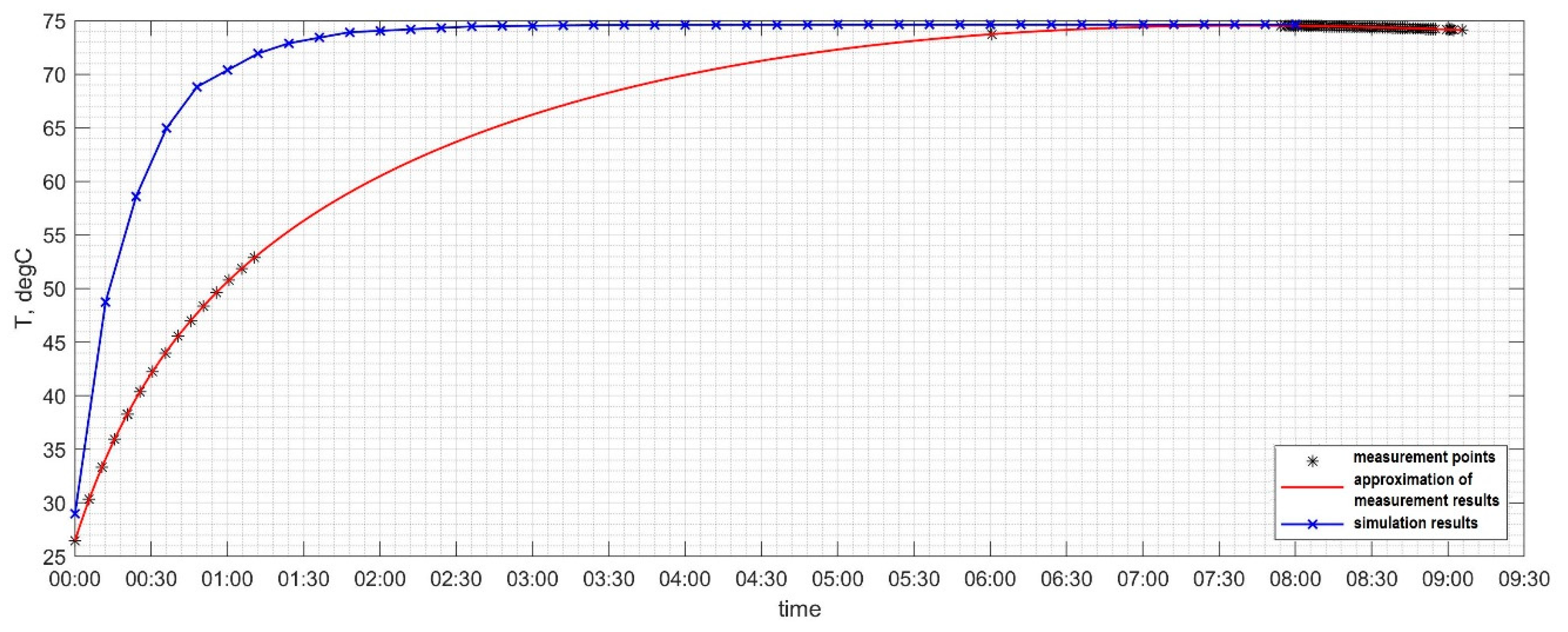
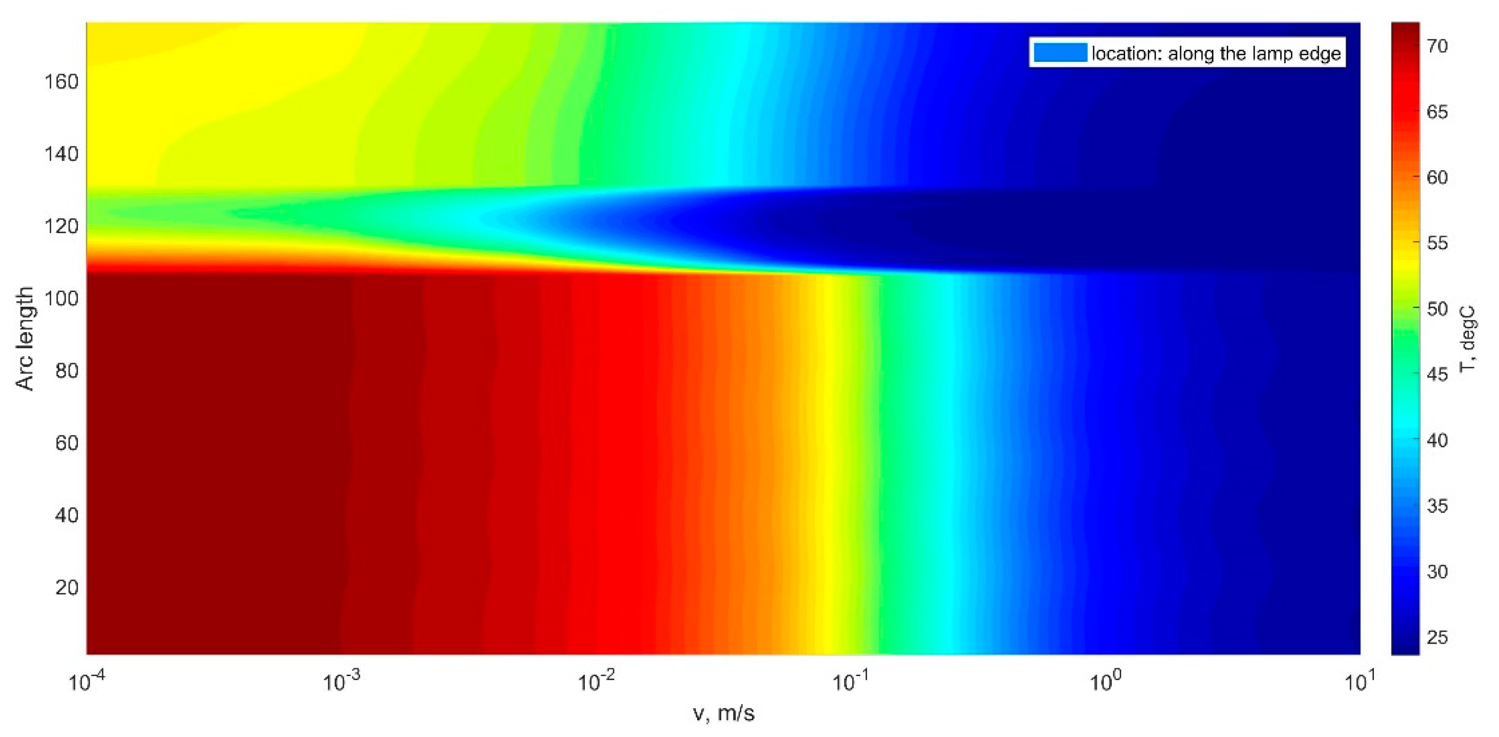
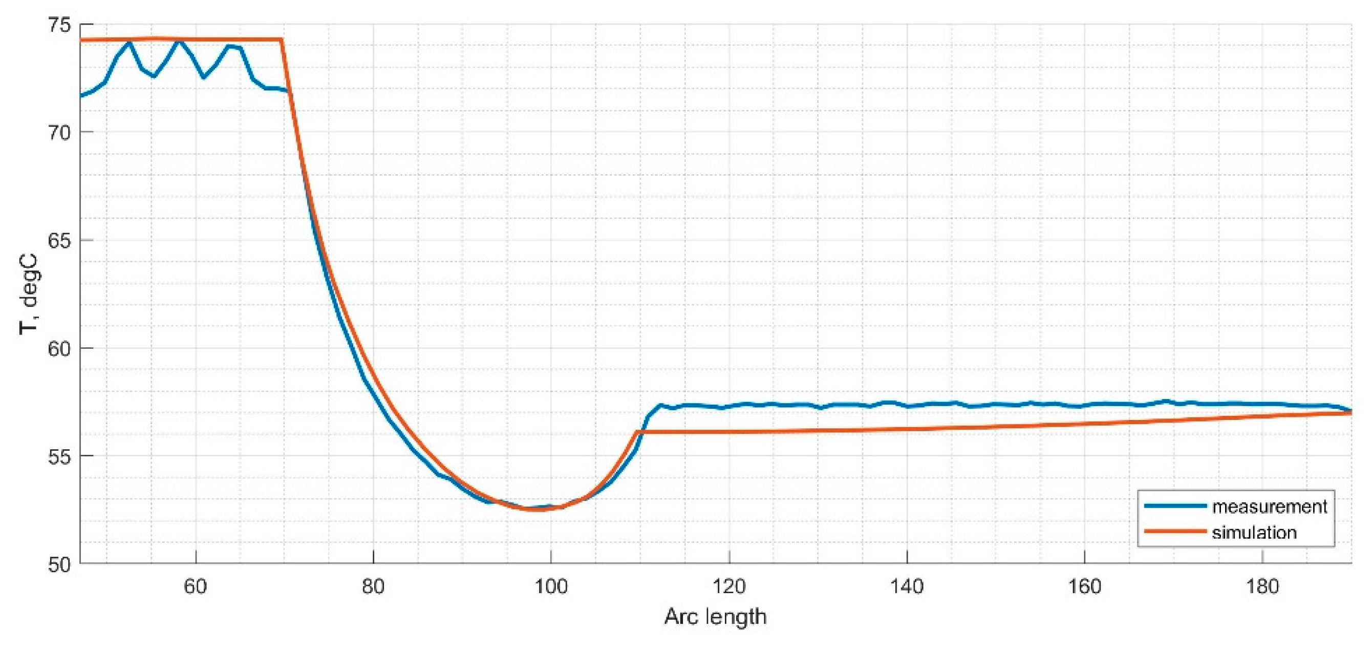
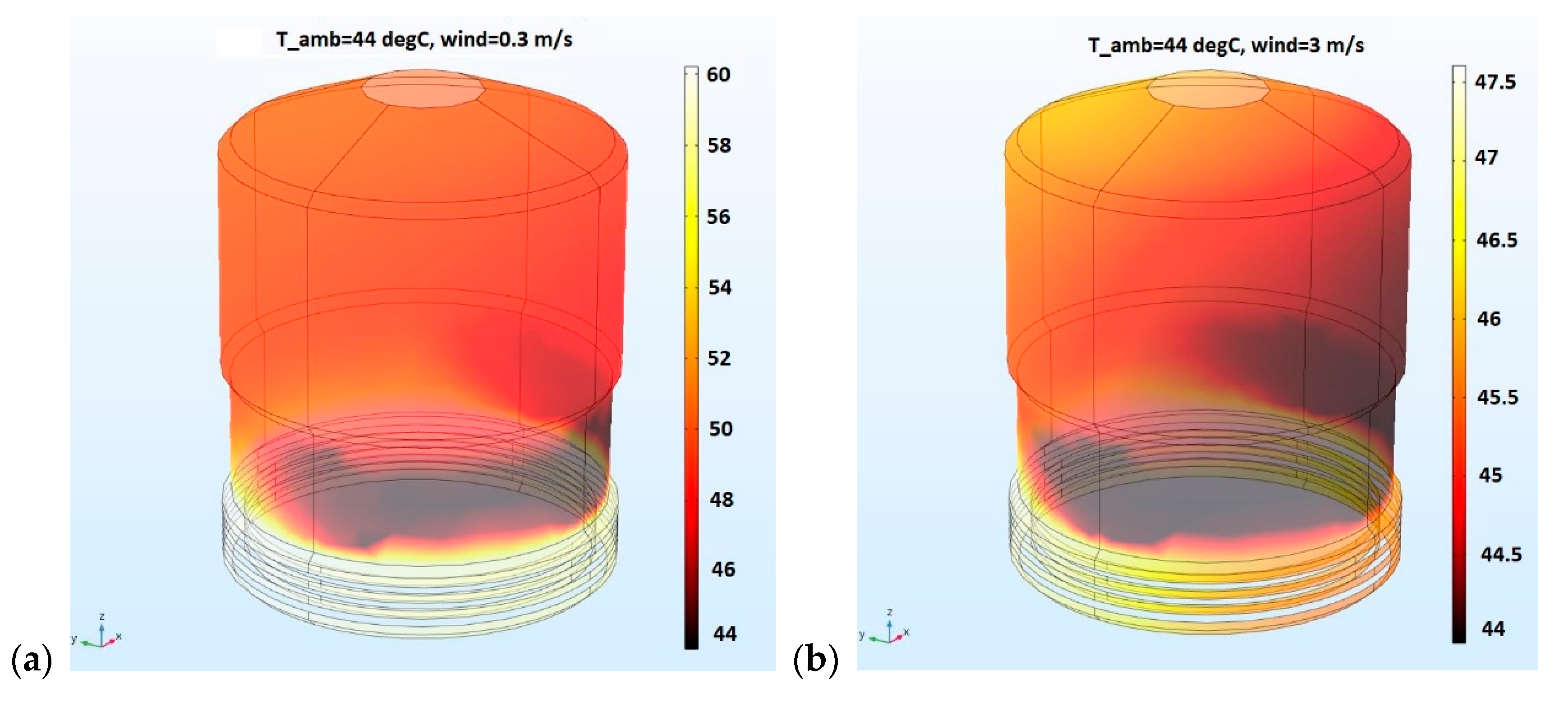
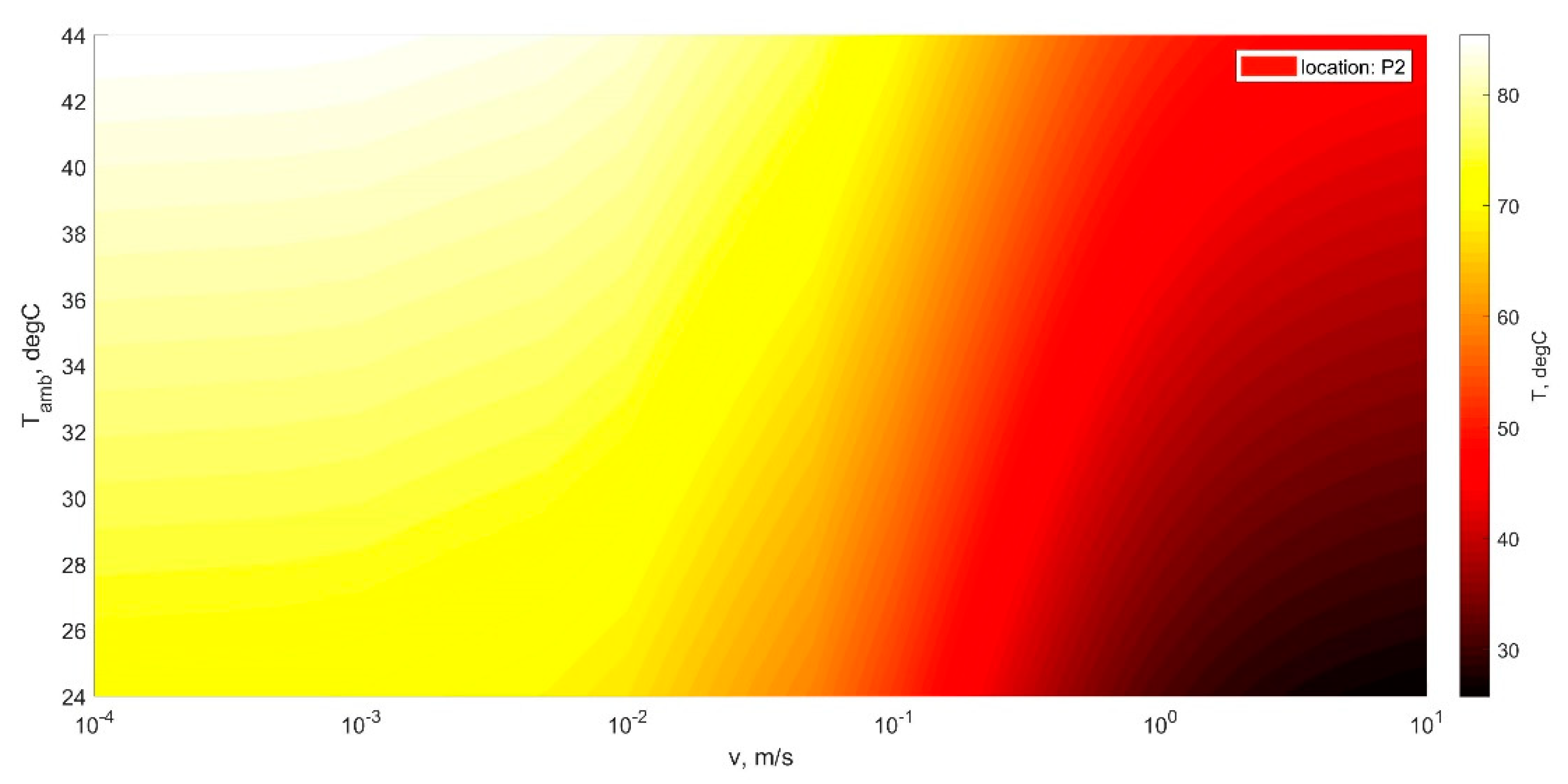
3. Measurement and Analysis Results

In the course of the experimental research works, several measurement sessions were conducted in which the heating process of the lamp was recorded with the use of the thermal imaging camera. The images were taken at such intervals that it was possible to draw the lamp heating curve and then to determine the trend using non-linear regression. Figure 3 depicts example images gathered at the very beginning, after six minutes of operation (Figure 3a), and in the stabilized state, after about seven hours of operation (Figure 3b). Based on the gathered images, it was stated that the temperature distributes equally within the two heat sinks. The values are higher on the bottom heat sink, which dissipates the heat produced by LEDs as at the top heat sink. The lowest temperatures were registered in the central part of the lamp, which is made of plexiglass. The temperature around the object decreases rapidly with the distance and targets the ambient temperature. In Figure 4a, the temperature distribution on the lamp surface after eight hours of operation gathered from the computer simulations is presented. The distribution of heat calculated for the lamp surface corresponds to data gathered from measurements. In order to assess the quality of the calculated model, temperature values that were registered and calculated along the edge of the lamp surface and at a point defined as P2, as depicted in Figure 4b, were compared.
In Figure 5, the verification result is presented, which depicts temperature values measured (in blue) and calculated using the numerical model (in red) along the edge of the lamp on its surface established after 8 h of operation, thus in the steady state. In general, the waveforms of the curves are consistent and overlap. There are inaccuracies visible in the lower part of the lamp, at the rungs of the bottom heat sink, where temperature fluctuations in the range of 2 °C were recorded with the thermal imaging camera, whereas in the numerical model, these fluctuations were not observed. The temperature difference in this area is of 2.7% with a maximum value of 74.5 °C. In the transparent area of the plexiglass, the temperature values do not differ significantly. The temperature difference in the area of the top heat sink equals a maximum of 1.5 °C, which by a temperature equal to 57.5 °C implies a 2.6% deviation between the measured and calculated values. The overall error does not exceed 3%; therefore, it was assumed that it can be neglected, and the model has been positively verified.
Figure 6 shows the transient and steady-state results of measurements and calculations. The values marked as black stars depict values gathered from thermal images and refer to the highest recorded temperature on the bottom heat sink. The values marked as blue crosses refer to temperatures calculated in the point P2 in the numerical model, which is located on the bottom heat sink. The values were achieved by ambient temperature Tamb = 28 °C and zero airflows. Analyzing the data presented in Figure 6, it is obvious that the numerical model of the lamp heats up much faster and that the steady state occurs after only three hours of the simulation time, while the actual model reaches the temperature saturation only after seven hours. This is the result of many simplifications adopted in the computational model, and is related to the fact that not all elements of the lamp were modeled, but only the key parts in terms of the geometry of the top and bottom heat sinks. However, despite this difference in the transient state, the temperature in the steady state is convergent in the model, as shown exemplary for the point P2.
The experimental data were interpolated using rational function f(t), which is given by Equation (13), obtaining suitable results and achieving the following fitting parameters: sum squared error (SSE) = 2.6273, root mean square error (RMSE) = 0.1824. The red line in Figure 6 depicts the approximation result.
f ( t ) = p 1 t 2 + p 2 t + p 3 t 3 + q 1 t 2 + q 2 t + q 3  
where t is time normalized by mean = 7.374e + 05 and std = 0.1264, and the coefficients (with 95% confidence bounds) are as follows: p 1 = 512.4 (−127.8, 1153); p 2 = 4350 (2651, 6050); p 1 = 7557 (6397, 8717); q 1 = 9.626 (1.703, 17.55); q 2 = 56.96 (33.8, 80.11); q 3 = 101.6 (85.88, 117.2).
On the basis of the results presented in Figure 5 and Figure 6, it was stated that the calculation model is positively verified, which allows for its application for further theoretical analyses. Therefore, in the next step, parametrical analysis was performed, in which the ambient temperature and the airflow velocity were changed and their influence on the temperature distributions was investigated. In Figure 7, an example of steady-state simulation results depicting temperature distribution at the lamp surface by Tamb = 44 °C and wind speed equal to v = 0.3 m/s and v = 3 m/s are depicted.
From Figure 7, it may be observed that the dependence of the ambient temperature is not linear, and the influence of air cooling is different for various ambient temperatures. The cooling effect is lower at higher ambient temperatures. The temperature on the lamp surface is distributed according to the direction of the air movement. The values depend on the velocity and the ambient temperature.
In Figure 8, the results of theoretical analyses for various values of Tamb and v in a wide range of changes that concern the steady-state temperature values in point P2 are presented. Please note that the scale is logarithmic for wind speed.
In Figure 9, the results of analyses for various wind speed changes concerning the steady-state temperature values calculated along the lamp edge by Tamb = 24 °C are presented. The influence of cooling is the lowest in the bottom heat sink and the highest in the transparent plastic part. At the highest cooling values, the differences become blurred, and so at v = 10 m/s, the temperature of the lamp surface drops to the ambient values.

4. Discussion, Future Work, and Conclusions

The measurement system used was designed to reflect and determine the conditions of lamp operation in various atmospheric conditions. It is much more difficult to perform measurements for all conditions, not to mention changing the geometry of the lamp to optimize its parameters. Therefore, the numerical model was developed, and its parameters and the boundary conditions used in the equations were adjusted in such a way that the results were consistent with the measurements. The experimentally verified numerical model was used for further analysis by changing the ambient temperature and wind speed values.
Based on on situ measurements, it was found that the temperature of the lamp stabilizes after approximately 7 h of operation, which corresponds to the average night-time operation in a moderate climate. However, the numerical model of the lamp reaches the steady state already after 3 h of operations, which was due to the great simplifications of the numerical model and the individual elements of the lamp having not been taken into account. Nevertheless, the steady state of both the computational and physical models agree in terms of the temperature distribution on the lamp surface. Moreover, the performed theoretical analyses allowed determining the heat emitted by the currently produced lamp at high wind speeds (up to 10 m/s) and for high ambient temperatures (up to 44 °C).
As part of future work, it is planned to analyze and change the shape of the heat sink in order to achieve better cooling results for high ambient temperatures and low wind velocities.
The advantage of the software used in research work enables the integration of various physical phenomena. In addition to the analysis of the interdependencies between air movement and heat emission, it is possible to extend the model in the future to include radiation emission and perform studies on the influence of heat emission on the propagating rays of light.

Author Contributions

Conceptualization, D.W., A.B., and P.W.; methodology, D.W. and P.W.; software, D.W.; validation, D.W., A.B. and P.W.; formal analysis, A.B.; investigation, D.W.; resources, A.B.; writing—original draft preparation, D.W.; writing—review and editing, A.B. and P.W.; visualization, D.W.

Funding

This research received no external funding.

Conflicts of Interest

The authors declare no conflict of interest.

References

  1. Ochoa, C.E.; Aries, M.B.C.; Hensen, J.L.M. State of the art in lighting simulation for building science: A literature review. J. Build. Perform. Simul. 2012, 5, 209–233. [Google Scholar] [CrossRef]
  2. International Civil Aviation Organization. Available online: https://www.icao.int/about-icao/Pages/default.aspx (accessed on 27 September 2019).
  3. Pérez-Ocóna, F.; Pozoa, A.M.; Rabazab, O. New obstruction lighting system for aviation safety. Eng. Struct. 2017, 132, 531–539. [Google Scholar] [CrossRef]
  4. Jianxin, Z.; Lixia, S. Modelling and Numerical Simulations of Heat Distribution for LED Heat Sink. Discret. Dyn. Nat. Soc. 2016. [Google Scholar] [CrossRef]
  5. Wu, S.J.; Hsu, H.C.; Fu, S.L.; Yeh, J.N. Numerical simulation of high power LED heat-dissipating system. Electron. Mater. Lett. 2014, 10, 497–502. [Google Scholar] [CrossRef]
  6. Zhao, X.J.; Cai, Y.X.; Wang, J.; Li, X.H.; Zhang, C. Thermal model design and analysis of the high-power LED automotive head light cooling device. Appl. Therm. Eng. 2015, 75, 248–258. [Google Scholar] [CrossRef]
  7. Lee, D.W.; Cho, S.W.; Kim, Y.J. Numerical study on the heat dissipation characteristics of high-power LED module. Sci. China Technol. Sci. 2013, 56, 2150–2155. [Google Scholar] [CrossRef]
  8. Ahmed, H.E.; Salman, B.H.; Kherbeet, A.S.; Ahmed, M.I. Optimization of thermal design of heat sinks: A review. Int. J. Heat Mass Transf. 2018, 118, 129–153. [Google Scholar] [CrossRef]
  9. Dong, X.D.; Ying, G.L.; Xiao, B.L. Numerical Analysis on temperature field in a LED module. Adv. Mater. Res. 2011, 221, 604–609. [Google Scholar] [CrossRef]
  10. Luo, X.; Cheng, T.; Xiong, W.; Gan, Z.; Liu, S. Thermal analysis of an 80 W light-emitting diode street lamp. IET Optoelectron. 2007, 1, 191–196. [Google Scholar] [CrossRef]
  11. Alexandersen, J.; Sigmund, O.; Meyer, K.E.; Lazarov, B.S. Design of passive coolers for light-emitting diode lamps using topology optimization. Int. J. Heat Mass Transf. 2018, 122, 138–149. [Google Scholar] [CrossRef]
  12. Vinh, Q.; Khanh, T.; Ganev, H.; Wagner, M. LED Lighting: Technology and Perception. Measurement and Modeling of the LED Light Source; Wiley Online Library: Hoboken, NJ, USA, 2014; Chapter 4. [Google Scholar] [CrossRef]
  13. Stüben, K.A. Review of algebraic multigrid. J. Comp. Appl. Math. 2001, 128, 281–309. [Google Scholar] [CrossRef]
  14. Schenk, O.; Gärtner, K. Solving unsymmetric sparse systems of linear equations with PARDISO. Future Gener. Comput. Syst. 2004, 20, 475–487. [Google Scholar] [CrossRef]
  15. Wagner, S. Small-Signal Device and Circuit Simmulation. Ph.D. Thesis, Technische Universität Wien, Vienna, Austria, 2005. Available online: http://www.iue.tuwien.ac.at/phd/wagner/diss.html (accessed on 10 September 2019).
Figure 1. A CAD drawing of the computational domain depicting the rectangular tunnel with the lamp and the lamps enlarged view (to the right).
Applsci 09 04951 g001
Figure 2. CAD drawing depicting the applied materials: (a) parts made of aluminum, (b) parts made of acrylic plastic, and the critical boundaries: (c) heat sources, (d) thermal insulation.
Applsci 09 04951 g002aApplsci 09 04951 g002b
Figure 3. Examples of images gathered from thermal imaging camera: (a) made after 6 min of operation; (b) made after 7 h of operation of the lamp.
Applsci 09 04951 g003
Figure 4. (a) Example image from simulation result depicting temperature distribution at the surface of the lamp in the steady state; (b) location on the edge of the lamp and at point P2 in the computational domain.
Applsci 09 04951 g004
Figure 5. Temperature values measured (in blue) and calculated using the numerical model (in red) along the edge of the lamp on its surface established after 8 h of operation.
Applsci 09 04951 g005
Figure 6. Results of measurements (in red) and simulation using the numerical model (in blue) gathered in the transient state during the heating process.
Applsci 09 04951 g006
Figure 7. Example simulation results depicting temperature distribution at the surface of the lamp in the steady state for Tamb = 44 °C and wind speed equal to (a) v = 0.3 m/s; (b) v = 3 m/s.
Applsci 09 04951 g007
Figure 8. Results of simulations performed using the numerical model depicting the calculated temperature values in dependence from wind speed (log scale) and ambient temperature (linear scale) values at location point P2 (see Figure 4b).
Applsci 09 04951 g008
Figure 9. Results of simulations performed using the numerical model depicting the calculated temperature values in dependence from wind speed (log scale) along the lamp edge (see Figure 4b) by ambient temperature Tamb = 24 °C.
Applsci 09 04951 g009
Table 1. Material parameters applied in the model.
DescriptionAluminumAirAcrylic Plastic
Heat capacity at constant pressure [J/(kg·K)]900Cp(T)1470
Thermal conductivity [W/(m·K)]238k(T)0.18
Density [kg/m3]2700rho(p, T)1190
OpacityOpaqueTransparentTransparent
Surface emissivity 0.96 (red paint)-0.15
The ratio of specific heats-1.4-
Diffuse surface-radiation directionsopacity controlled-on both sides
Table 2. Mesh settings for the tunnel (T), the lamp (L), and its vicinity (V).
DescriptionValue for TValue for LValue for V
Maximum element size141 [mm]308 [mm]308 [mm]
Minimum element size42.4 [mm]13.2 [mm]13.2 [mm]
Curvature factor0.70.30.3
Resolution of narrow regions0.60.850.85
Maximum element growth rate1.21.351.35
Table 3. Mesh statistics.
DescriptionValue
Minimum element quality0.02403
Average element quality0.6615
Tetrahedral elements169,568
Triangular elements13,294
Edge elements1760
Vertex elements121

