Abstract
The objective of this paper is to investigate the complete process of dynamic crack propagation in brittle materials under different loading rates. By using Improved Single Cleavage Semi-Circle (ISCSC) specimens and Split Hopkinson Pressure Bar equipment, experiments were conducted, with the fracture phenomenon and crack propagation of tight sandstone investigated. Meanwhile, the process of crack propagation behaviour was simulated. Moreover, with the experimental–numerical method, the crack propagation dynamic stress intensity factor (DSIF) was also calculated. Then, the crack propagation toughness of tight sandstone under different loading rates was investigated and illustrated elaborately. Investigation results demonstrate that ISCSC specimens can achieve the crack arrest position unchanged, and the numerical simulation could effectively deduce the actual crack propagation, as their results were well matched. During crack propagation, the crack propagation DSIF in the whole process increases with the rising loading rate, and so does the crack propagation velocity. Several significant dynamic material parameters of tight sandstone are also given, for engineering reference.
1. Introduction
Rock mass contains plentiful joints, fractures, and crevices with different sizes and shapes, presenting complex heterogeneous formations. Under impact loads, these defects will initiate, propagate and evolve [1,2,3,4,5]. In geotechnical engineering practice, such as mining, tunnelling and deep-earth engineering, impact loads as an engineering approach have been widely utilized for rock breakage and destruction [6]. It is essential to predict crack propagation velocity, path, dynamic stress intensity factor and behaviour, in order to deploy a rational strategy for engineering design and hazard mitigation. Therefore, a complete study on rock dynamic crack propagation under different loading rates is of profound importance.
In previous decades, the whole process of failure characteristics in pre-existing crack rock mass under impact loading has been discussed in many research works. Numerous research works based on experimental laboratory testing have been conducted to understand the mechanism [7,8,9,10,11,12,13]. Hitherto, studies have already demonstrated the importance of selecting a specimen with a suitable configuration during studies on rock fracture mechanics. Until now, many specimen configurations have been proposed and applied in investigations, such as Cracked Straight-Through Flattened Brazilian Disc (CSTFBD) [14], Semi-Circular Bending (SCB) [15], Single Cleavage Drilled Compression (SCDC) [16], Single Cleavage Semicircle Compression (SCSC) [17], etc. Those specimens had different advantages in the investigation of crack behaviour, including crack initiation, crack arrest, extended angle effects and crack initiation toughness. However, they were rarely applied to study the complete process of dynamic crack propagation quantitatively, as the suitability of most of these type of samples is controlled and limited by their size. For this purpose, a new specimen, which can be employed in investigating the complete process of dynamic crack propagation behavior, and measuring a whole range of crack propagation dynamic stress intensity factors (DSIF), is needed.
The rock crack propagation mechanism is more complicated than the static crack mechanism. Ravi-Chandar et al. [18] studied the dynamic crack propagation phenomenon and laws of crack propagation under impact loads. They have shown that cracks propagate rapidly under constant velocity, even though the stress intensity factor varies considerably during propagation, and crack arresting occurs abruptly with discontinuous deceleration. Then, Eberhardt et al. [19] carried out a study to investigate details of crack initiation and propagation thresholds and proved that crack propagation can be in either stable or unstable conditions, depending on stress threshold. Later, the effect of heterogeneity in rock material on crack fracture propagation was also studied. Then, Gregoire et al. [20] focused on pre-crack propagation behaviour under impact loading, and their investigation revealed that crack propagation could stop and restart during the whole propagation process. Gao et al. [21] probed into the influence of loading rates on fracture propagation behaviour with NSCB samples, while Chen et al. [22] obtained crack initiation toughness and propagation behaviour toughness with an Split Hopkins Pressure Bar (SHPB) experiment system. With the aid of laser technology, Yang et al. [23] employed the digital-laser dynamic caustic system to investigate the crack propagation under the effect of a circular defect, unveiling that the crack path deviates towards the defect that existed in the vicinity of the crack path. Wang et al. [17] investigated the crack propagation of sandstone with SCSC specimen by using Split Hopkinson Pressure Bar test system and tried to observe crack arrest phenomenon, but the crack arrest position of this configuration is variable. However, most research focused on crack initiation and propagation as well as DSIF, and was less concerned about studying crack behaviour in a complete process, including its initiation, propagation and arrest, and even its stop.
Under impact loading, the mechanical behaviour of fracturing specimen presents a complicated state, as material physical parameters change significantly with loading rates [24,25]. Sometimes the tensile strength of material increases by 6–8 times, even exceeding to nearly an order of magnitude [26]. With well-established computational techniques, combined with the actual experiment, an experimental–numerical method is introduced into the research of crack fracture mechanisms and crack propagation. Therefore, the physical experimental results could be validated, and crack extension could be well predicted through computational techniques. A finite difference code (AUTODYN) has demonstrated great superiority in solving multifarious problems characterized by both geometric nonlinearity and material non-linearity, performing elegantly in investigating crack propagation in the complete process [27,28,29,30].
In this paper, an improved single cleavage semi-circle specimen was applied. Meanwhile, impact experiments were carried out to investigate the rock crack propagation phenomenon with the validity of the configuration verified. Moreover, the effect of loading rate on crack propagation behaviour was considered as a significant factor. In order to study the crack propagation velocity, the crack propagation gauge (CPG) test system was employed. Then, a suitable numerical simulation model was established by using a tensile crack softening law [31]. Some comparative studies between experiments and simulations were carried out to verify the modelling approach and to check its level of accuracy. At last, an accurate numerical simulation with ABAQUS finite element code figured out the crack propagation DSIF of the whole process [32]. Therefore, the present paper demonstrates a method to determine the crack propagation dynamic stress intensity factor in the whole process, which provides the reference data for practical projects to deploy a rational strategy for engineering design and hazard mitigation. Notably, the loading rates’ effect on crack propagation and DSIF has significant meaning for engineering applications attempting to deal with the problems related to loading impact change. Moreover, the investigation of the crack propagation behaviour and the influence of holes on the extending crack illustrates the physical mechanism of a practical phenomenon in engineering projects. It also provides some insights into the crack propagation process, as well as proposing an innovative crack arrest technique to take advantage of this with regards to tunnelling and deep earth engineering. The experimental and numerical simulation investigation method, which can be utilized to measure the mechanical parameters of brittle material, can be applied in civil engineering for further research.
2. Material and Experiment
As a significant material in engineering application, black sandstone was chosen, with its crucial dynamic mechanical property investigated. The propagation behaviours of pre-crack on the black sandstone specimen were focused on, and ISCSC specimen configuration, along with the test system, is introduced in detail.
2.1. Material
YaMeng black sandstone, a kind of sedimentary rock with dense density and high strength mechanical properties, which has an important research significance in engineering applications, was selected to be investigated, and forms the specimens. Under the camera of an electron microscope, the particles of black sandstone are uniformly distributed, the grain sizes are approximate, and pores are less, as shown in Figure 1. Therefore, with the physical properties of the material, size effect related errors, which are generated when rocks with broad particles aggregate distribution, were reduced when investigating crack propagation characteristics. The longitudinal and transverse wave velocity of the samples was measured by a non-metallic acoustic detector. Then, the dynamic elastic modulus and dynamic Poisson’s ratio was calculated by Equations (1)–(3) [33]. The crucial dynamic parameters of YaMeng black sandstone are listed in Table 1.
where cd is longitudinal wave velocity, cS is transverse wave velocity, cR is Rayleigh wave velocity, Ed is dynamic elastic modulus, νd is Poisson’s ratio, ρ is density.

Figure 1.
Micrographs of YaMeng black sandstone by Scanning Electron Microscope (SEM) (a) The micrograph with scale of 50.0 μm. (b) The micrograph with scale of 10.0 μm.

Table 1.
Material parameters of YaMeng black sandstone.
2.2. SHPB Test System
In impact experiments, A Split Hopkinson Pressure Bar [34] was employed, as shown in Figure 2. The length of the impact bar, the incident bar, and the transmitted bar are 400 mm, 3000 mm and 2000 mm, respectively, and the diameters of the bars are 80 mm. The material parameters of the incident bar and transmitted bar made by 40 CrmoV alloy are listed as follows: density is 7 600 kg/m3, the elastic modulus is 210 GPa, Poisson’s ratio is 0.25 and the longitudinal wave velocity measured is 5164 m/s. The voltage signals, recorded from the strain gauges deployed in the middle of the incident bar and the transmitted bar, respectively, and crack propagation gauges glued on the specimens, were collected by ultra-dynamic strain amplifier, then stored in a digital oscilloscope. Furthermore, voltage signals could be converted into strain signals after noise reduction operation. The impact velocity of the impact bar was measured by the photoelectric velocity acquisition system. A waveshaper, a piece of purple copper of coin size, was employed in the experiment for the purpose of obtaining the ideal wave, as it has the function of attenuating the diffusion effect of a stress wave and reducing the oscillation effect of high-frequency stress waves.
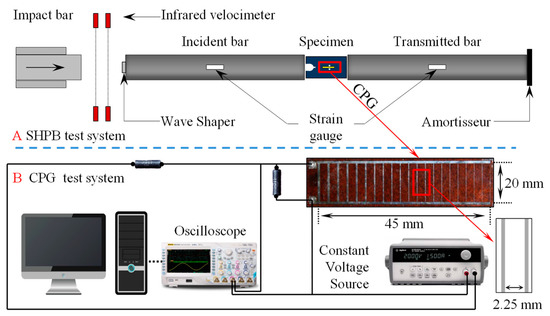
Figure 2.
Schematic of the Split Hopkins Pressure Bar (SHPB) test system and crack propagation gauge (CPG) test system.
The crack propagation gauges (CPG)s were applied in the experiment, and the CPG test system is illustrated in Figure 2. CPG, which is a kind of gauge made up of a glass–silk baseplate with fine wires equispaced on it, was used to measure the velocity of the running crack. During the experiment, the CPGs were tightly glued on the surface of specimens, and the area that they were located on was large enough to cover the conceivable crack propagation path. During the crack propagation process, the wires break one by one as the crack propagates. Then, the total resistance of the CPG and the voltage signal associated changes accordingly. Once the fine wire is fractured, the voltage signal at that moment changes sharply in response. This means that the voltage signal curve presents a step-by-step growth trend, which could be used to identify the location of running crack tip at a certain moment. Therefore, after analyzing the voltage signal data, the derivative of the voltage with respect to time could be obtained, and the time corresponding to the extreme derivative value was the moment when the running crack tip arrived. Based on the above principles, the average velocity of a moving crack between two fine wires which had a fixed distance of 2.25 mm could be calculated according to the gaps between the two fine wires and the fracture time.
2.3. ISCSC Configuration
The ISCSC specimen with rational configuration and excellent applicability was invented to investigate the crack propagation in the complete process, and its schematic is shown in Figure 3. The ISCSC specimen configuration presented advantages in the conducted impact experiment, as it caused the pre-crack to initiate easily and had the potential to give the running crack sufficient space to extend and arrest. So, the whole process of propagation could be observed distinctly, and many characteristics of fracture behaviour could be detected precisely. Meanwhile, a particular set area where crack arrest would occur was created by deploying a pair of symmetrical empty holes on the specimen, so detailed information on the crack arrest could be traced and investigated.

Figure 3.
Improved Single Cleavage Semi-Circle Specimen (ISCSC) specimen sample geometry.
Geometric parameters of the specimen are listed in the following: 145 mm length, 70 mm width, 35 mm thickness, 22 mm diameter of semi-circle, and 30 mm length of pre-crack whose tip was sharpened with a thickness of 1 mm. Two pre-set empty holes located on both sides of the central axis of the specimen symmetrically, with a 6 mm diameter and 18 mm distance of the centre of the two holes. The distance between the location of the pre-crack tip and the midpoint of the centre of two holes was 40 mm.
2.4. Experiment Results and Analysis
In order to avoid the results being disturbed by external factors and random error, twenty specimens with ISCSC configuration were employed and impacted with different speeds, from 6.0 m/s to 8.5 m/s. According to the laws of processing data, the data were filtrated and the signals collected from the experiment were analyzed.
Based on the voltage signals recorded by the strain gauges, the strain signals could be converted with Equation (4):
where ε is the strain, U0 is the voltage recorded by strain gauges, Eg is the bridge voltage, K is the sensitivity coefficient of the strain gauges, and n is the gain coefficient of an amplifier.
Then, the loads acting on the top and bottom of the specimen could be calculated with Equation (5), and their curves of loads versus time are shown in Figure 4a.
where εi(t) and εr(t) are the strains of incident bar caused by incident wave and reflected wave, εt(t) is the strain of transmitted bar caused by the transmitted wave, Pi(t) is the loads on the top of the specimen and Pt(t) is the loads on the bottom of the specimen.
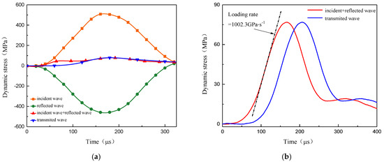
Figure 4.
Curves of loads versus time (a) The dynamic stress curves detected from the incident bar and transmitted bar. (b) Determination method of the loading rate.
According to the curves of the loads detected in different tests, the maximum loading rate of each experiment could be obtained technically by utilizing Origin software, as Figure 4b shows. Thus, three typical crack propagation patterns in the experiment were selected, each with a different maximum loading rate—1000 GPa·s−1, 1500 GPa·s−1, and 2000 GPa·s−1, respectively. The incident and reflected waves which were used to calculate the loading rate and the transmitted wave in Figure 4b are the waves obtained in the incident and transmitted bar showing stress equilibrium condition. However, the specimens in this experiment didn’t satisfy the dynamic force equilibrium condition. We agree that it is a critical step to determine whether or not the test meets the dynamic force equilibrium condition in the SHPB experiment. Assuming that the stress/strain of the specimen is uniformly distributed along its length, its purpose is to decouple the stress wave effect and strain rate effect. It is the basic assumption of the quasi-static method. But, in this paper, the ISCSC specimen was mainly employed to investigate crack propagation behaviour and loading rate effect, whereas the numerical method was introduced to continue the thorough research. The whole research method is a hybrid experimental–numerical approach [35], and it is already beyond the scope of quasi-static study. Therefore, it is not necessary to satisfy the assumption of the stress balance.
Figure 5 presents three typical crack propagation patterns of specimens in the experiment. The crack propagation paths on the specimen HT-1, HT-2, and HT-3 in Figure 5 were in a straight line before the running crack reached the two holes’ zone, where two empty holes were deployed, which accorded with the feature of mode I of fracture. As the running cracks went across the two holes area, the surfaces of two empty holes were damaged at different levels, with secondary cracks appearing around the two empty holes. The microstructure of the rock material played a crucial role in dominating the crack initiation and propagation, helping the running crack behave as shown above. It was found that the crack path would stay in the middle of the specimen if the rock material were homogeneous, as Figure 5b,c showed, or the crack path might perform as in Figure 5a. The crucial phenomenon related to this experiment is the dramatic change in crack propagation direction at the moment that the running crack drives into the two hole zone.
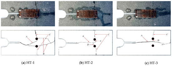
Figure 5.
Crack propagation patterns of Improved Single Cleavage Semi-Circle Specimen (ISCSC) specimens (a) The crack pattern of HT-1 specimen. (b) The crack pattern of HT-2 specimen. (c) The crack pattern of HT-3 specimen.
Figure 6 presents the voltage signal data and the derivative of the voltage, concerning the time recorded from CPG gauges on the specimens and curves of running crack velocity. As mentioned before, the time corresponding to the extreme value of the derivative of voltage is the moment when a fine wire of CPG fractured. Therefore, the average propagating velocity between adjacent wires could be calculated by constant distance 2.25 mm divided by fracture time. The average propagating velocity curves in green are plotted to show the significant trend of crack velocity. The specific points at which propagating speed changed significantly are chosen to divide the whole propagation process into different zones. In each zone, the average crack propagating velocity is given.
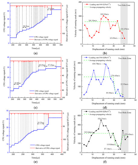
Figure 6.
Voltage signal and derivative, with respect to time recorded from the crack propagation gauge (CPG) and crack propagation velocity. (a) The CPG voltage signal of HT-1 specimen. (b) The crack propagation velocity curves of HT-1 specimen. (c) The CPG voltage signal of HT-2 specimen. (d) The crack propagation velocity curves of HT-2 specimen. (e) The CPG voltage signal of HT-3 specimen. (f) The crack propagation velocity curves of HT-3 specimen.
For the HT-1 specimen with loading rate 1000 GPa·s−1, shown in Figure 6b, when the running crack had grown to 25 mm, the crack propagation speed began to decrease. When the running crack grew to 35 mm, the crack decelerated rapidly, and the instantaneous position of the crack tip was 5 mm ahead of the connecting line of the two hollow holes. The maximal fracture time interval of the adjacent fine wires appeared between the 18th and 19th fine wire within 31.62 microseconds. The average crack propagation speed between the 18th and 19th wire was 63.69 m/s, which was the minimum speed of the running crack.
For the HT-2 specimen with loading rate 1500 GPa·s−1, as shown in Figure 6d, when the running crack reached 25 mm, the crack propagation speed began to decrease and decelerated rapidly without hesitation. Moreover, the maximal fracture time interval of adjacent fine wires appeared between the 17th and 18th fine wire within 87.22 microseconds. This time was already beyond the average fracture time intervals of the whole fine wires, as well as the theoretical maximal fracture time interval of 60 microseconds, given by Wang et al. [17]. This time interval was considered as a standard to identify the time that the crack arrest phenomenon occurred if the fracture time interval of adjacent fine wires of CPG becomes longer than 60 microseconds. Also, the average crack propagation speed at 38 mm was 22.97 m/s, which could be further proof that crack arrest had occurred in this area.
After the fracture of the 18th fine wire, the rest of the fine wires’ voltage signal was steadily detected by CPG, which shows the running crack had stopped between the two holes until transverse cracks occurred.
For the HT-3 specimen with loading rate 2000 GPa·s−1, as shown in Figure 6f, the displacement at which the deceleration of the running crack occurred was 20 mm. After that, the velocity of the running crack reduced continually to reach the minimum speed, 57.14 m/s, and the velocity of the running crack had increased when the crack passed the set area between the two holes. The maximal fracture time interval of adjacent fine wires appeared between the 16th and 17th fine wire within 35.23 microseconds.
As mentioned above, the running cracks on specimens performed similarly; the deceleration phenomenon appeared when the crack drove into the two hole zone, and arrest occurred in the propagation process. Moreover, judging from Figure 6, the average velocity and the maximum velocity of running crack were increased with the enhancement of the loading rate. It is prominent that the phenomenon in which the speed of running crack decayed rapidly appeared earlier with a rise in loading rate.
Then, a more in-depth analysis was conducted by considering the crack fracture appearances. For the HT-1 specimen, as Figure 5a shows, the three zones where crack fracture appearances present different characteristics are marked with A, B, C. Based on the conclusions above, the running crack propagated in Zone A and arrested in the set area between two holes. For the cracks in Zone B, although the initiation time of the crack can’t be directly measured by gauges, the cracks should propagate along with the main crack as a way to release energy, which is also the reason why the crack in Zone A stopped. After the crack in Zone A stopped, the cracks in Zone B continuously propagated until the crack tip reached to the bottom of the specimen. Compared with the other specimens in the experiment, the appearance of the cracks in Zone C showed a disturbance, as the cracks were produced by the secondary impact, which can be ignored.
For the HT-2 specimen, as Figure 5b shows, with a higher loading rate, the main crack in zone A is straighter than in HT-1, and no secondary crack appeared in Zone B. Instead a crack appeared in Zone D, which could be shaped by the secondary impact. This is because, if the crack in Zone D was produced by the initial effects, the crack would propagate directly to the main crack and the bridge arm of CPG would break down, causing the CPG system to stop working immediately, which would mean the voltage signal from the 16th to 18th wire couldn’t be recorded. As the CPG voltage signal from 16th to 18th could be detected, there is crucial evidence to support the aforementioned assumption. Therefore, regarding to the crack in Zone D in the HT-3 specimen, the conclusion is the same. However, the crack in Zone E was shaped by the evolved main crack; when the arrested main crack between the holes restarted, the running crack tip drove to the hole and stopped.
For the HT-3 specimen with loading rate 2000 GPa·s−1, the performed crack appearance is very concise; the main crack went across the whole specimen, along with the symmetry axis. The secondary impact shaped the cracks in Zone C and D.
Detailed information can be achieved by comparing the three crack patterns. For example, the main reason that the running crack changes direction and drives directly towards a hole when the main crack runs closer to the hole can be understood, as HT-1 in Figure 5a shows. Also, the contrast in the crack patterns suggests that the main crack would restart and propagate continually with a straight line arrestment if the energy is large enough (as shown in the HT-3). Or it may run into an area where the material is easier to fracture. It can be inferred that the empty hole has an attraction effect on the nearby running cracks.
3. Numerical Simulation
The numerical code AUTODYN was applied to obtain quantitative results of crack propagation in the whole process, as well as study the mechanism of the crack arrest in a set area. The AUTODYN has been widely used because of its powerful ability in solving multifarious problems. It has been used especially for solving the problems of deformation and damage failure in rock material.
3.1. Numerical Simulation Model
YaMeng black sandstone is a typical brittle material with very small volume deformation under impact loading in the experiment, therefore the linear equation of state was applied to describe the material deformation, expressed by Equation (6):
where P is pressure, κ is bulk modulus, ρ is the current density of rock and ρ0 is the initial density of the rock.
The crack propagation of YaMeng black sandstone under impact loading is a gradual process, with the micro-cracks in the crack tip initiating, gathering, growing and shaping the macroscopic crack. Consequently, the maximum tensile strength failure model is chosen as the fundamental criteria, along with the tensile fracture softening damage criteria. When the maximum principal stress σ11 is higher than the maximum dynamic tensile strength σmax, the micro-cracks of the element will initiate, and then the tensile fracture softening damage criteria could describe the material damage failure process as accurately as possible. The Equations (7) and (8) are shown as follows to express the damage mode:
where D is the damage factor, εcr is the fracture strain, εu is the total fracture strain, σT is the maximum dynamic tensile strength, L is the characteristic dimension in the direction of maximum principal stress of the element, Ge is the fracture energy and σmax is the bearing maximum principal stress. In addition, the bearing maximum principle stress will keep going down to zero. The fractured element can still maintain the capacity to withstand compression and shear loads, but not tensile loads.
Figure 7 shows the numerical simulation model of ISCSC specimens, established according to the geometric dimension in Figure 2. With reference to the results of the experiment, three crucial areas are focused on as their meshes are specially designed and elaborately divided. Two rows of elements with length 0.1 mm were deployed from the pre-crack tip, along with the predicted crack propagation path to the bottom of the specimen, to realize randomness of crack initiation as well as to simulate crack propagation path precisely. Meanwhile, a relatively fine mesh was generated in the two hole area to monitor the change of the stress field in this area. The material parameters and loads applied in this simulation are based on the measured results from the experiment, as shown in Figure 4 and Table 1.
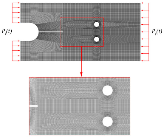
Figure 7.
Mesh of the ISCSC specimen.
3.2. Numerical Simulation Results
The simulation results of the crack propagation path are shown in Figure 8. As three loading rates are applied in the numerical simulation, the crack propagation path performs some universality appearances as well as some difference in detail. It is clear that the main crack runs straight after pre-crack initiation and across the set area before it stops at the back of it. Meanwhile, secondary cracks emerge on the holes, which present different fracture phenomena, as the secondary cracks on the back surface of both holes have a larger fracture area than the front ones, and the crack propagation path of the hole below is longer than the above. Also, the transverse crack emerges on the two sides of the hole, as HT-2 and HT-3 in Figure 8 show.
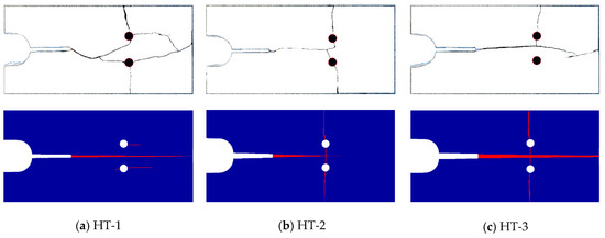
Figure 8.
Simulation results of crack propagation paths calculated by AUTODYN. (a) Comparison of specimen HT-1 between numerical simulation and experiment. (b) Comparison of specimen HT-2 between numerical simulation and experiment. (c) Comparison of specimen HT-3 between numerical simulation and experiment.
When comparing those fracture phenomena with the experimental results, the simulation results show a significant similarity with the results of the specimens in the experiment shown in Figure 8. It can be clearly seen that their main cracks all cross the set area along with the secondary cracks emerging on both sides of the holes. Especially with the high loading rate and the secondary impact, the transverse cracks on both sides of the holes are generated sufficiently within the expected time.
Despite the points discussed above, the fracture phenomenon in the specimens, where the running crack rushes directly into the hole below (shown by HT-1 in Figure 5a), is hardly reproduced by the numerical simulation. This is because the sandstone employed in the experiment is not the perfect homogeneous material which contains many irregular fissures and particles, offering a lot of tunneling opportunities when the cracks initiate and propagate. During the propagation process, the running crack might deviate from the symmetry axis of the specimen and approach the hole, resulting in the influence of the hole leading the running crack to rush directly into the hole. However, the material given in the numerical simulation is the ideal homogeneous material, so the cracks could run straight along the symmetry axis of the specimen, leaving no chance for the running crack to approach the hole.
Therefore, the comparative analysis is conducted between the numerical simulation, using the experimental results specimen as the calibration reference, to investigate the crack propagation behaviour and mechanism of arrest in the set area.
3.3. Numerical Simulation Analysis
To investigate crack propagation velocity, a group of gauge points is sown on the simulation specimen. Each has the same location, in line with the fine wire of the CPGs. The time when the running crack tip arrives at the gauge point can be obtained automatically. Then, the crack propagation velocity of simulation can be calculated by the velocity formula, where average velocity between two gauge points is equal to distance divided by time, as the distance between two gauge points is constant and equal to 2.25 mm.
Figure 9 shows the crack propagation velocity curves obtained by numerical simulation under three loading rates’ impact. It is seen that the crack propagation speed in both simulation and experiment has a highly consistent change trend. After initiation, the speed of the running crack increases with time inconstantly, while the propagating speed decelerates sharply when the running crack approaches the two hole zone. It is observed that the average speed of the main crack in the simulation has a relationship with the loading rate. With a higher loading rate, the average propagating speed of the HT-3 specimen, 443.07 m/s, is faster than the HT-1 specimen, with velocity 394.97 m/s. Comparing with Figure 9a,c, the fluctuation of propagating crack velocity under a high loading rate is more drastic than in the one with a low loading rate. Meanwhile, under a high loading rate, the deceleration of the propagating velocity is more sensitive. In other words, the two hole zone has a more dominant influence on running crack under a higher loading rate.

Figure 9.
Contrast diagram of crack propagation velocity under different loading rates (a) The crack propagating velocity curves of HT-1 specimen under loading rate 1000 GPa·s−1. (b) The crack propagating velocity curves of HT-2 specimen under loading rate 1500 GPa·s−1. (c) The crack propagating velocity curves of HT-3 specimen under loading rate 2000 GPa·s−1.
Therefore, the influence of the two hole zone should respond to dynamic crack propagation behaviour. For this purpose, a narrow study, focused on the two hole zone, is conducted to reveal the effect of the two empty holes on the crack propagation behaviour.
Figure 10 shows three significant moments of the process, where main cracks cross the two hole zone, with their particle velocity vector contour plotted. When t = 294.2 μs, the main crack tip arrives in front of the two hole zone with a very high speed, and then velocity declines immediately, according to previous analysis. From Figure 10a, it is evident that the surface of the two empty holes has a distinct deformation, transforming the circle to an ellipse, as shown in Figure 10d. This is because, when the incident stress wave arrives in the two hole area, the stress wave reflects on the front surfaces of the holes’ shaping reflected tensile wave, and the compressive wave reflected from the bottom of the specimen works on the back surfaces of the holes. These contribute to the deformation of the two holes. It is the deformation of the two empty holes that prompts the particles between two holes to move toward the symmetric axle of the specimen and shapes a compressive stress field between them. This compressive stress field plays a crucial role in reducing the velocity of the running crack.
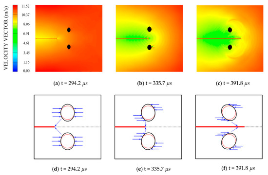
Figure 10.
HT-1 specimen; (a–c) simulation results of the particle velocity vector contour plot calculated by AUTODYN; (d–f) principle diagram of the holes’ deformation.
As the dynamic crack propagation continues, the free surface of the dynamic crack collaborates with the boundary of two empty holes, reshapes stress wave distribution, and results in transforming the curvature of ellipse shown in Figure 10e,f, which, in response, causes the direction of particles moving between two holes to change with time and leads the compressive stress field to have different effects on the running crack. For instance, when t = 335.7 μs, the compressive stress field has a strong impact on the arresting running crack, during which the running crack may stop, as HT-2 in Figure 5b shows. However, when t = 391.8 μs, this stress field might facilitate crack propagation, enhancing the velocity of the running crack, with Figure 9a providing evidence that the crack propagation speed increases after the running crack goes across the two holes’ zone. Also, the compressive stress contour is extracted from numerical simulation and plotted in Figure 11 with the dynamic crack path at the corresponding time.
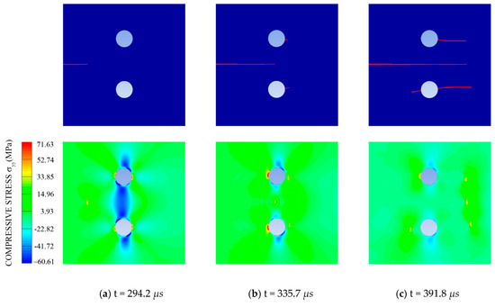
Figure 11.
Numerical simulation results of crack propagation paths and contour plot of the compressive stress calculated by AUTODYN. (a) The compressive stress contour plot when t = 294.2 μs. (b) The compressive stress contour plot when t = 335.7 μs. (c) The compressive stress contour plot when t = 391.8 μs.
Figure 11 illustrates directly that the compressive stress field exists between two holes and the intensity of the compressive stress field near the holes is higher than in other zones. Meanwhile, this compressive stress field presents most obviously when the running crack tip is in front of the two hole zone. If the crack pierces the two hole zone, the compressive stress field would be influenced by the tensile stress field around the main crack tip, as shown in Figure 11. When t = 335.7 μs and t = 391.8 μs, the two stress fields overlap with each other, reconstruct the whole stress field and dominate the crack propagation. The secondary cracks initiate on the back of the surfaces of the holes when t = 335.7 μs, while they appear on the front of surfaces when t = 391.8 μs. As the main crack has gone through the centre of the two holes, the secondary cracks on the back surface of the holes generate more actively as the tensile stress field become stronger than before. Thus, with the influence of the compressive stress field between the two holes and the secondary cracks, which share the energy required for the main crack propagation, the main crack propagates with very low speed.
In order to quantitatively illustrate the effect of the compressive stress field and its relationship with loading rate, the maximum compressive stress of twenty-one gauge points is detected from numerical simulation results, and the curves of the maximum compressive stress of three typical loading rates are plotted in Figure 12.
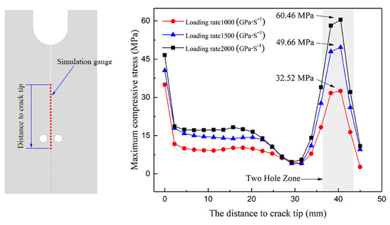
Figure 12.
Location map of gauges and maximum compressive stress curves of gauge points.
According to the compressive stress curves in Figure 12, it can be concluded that the intensity of compressive stress in the two hole zone is much greater than the rest of the gauge points during the stress wave’s progress in the specimen, and the maximum compressive stress appears at the center of the holes. Particularly, the maximum compressive stress monitored by gauges presents an entire increase tendency with the increase in loading rate. The maximum compressive stresses under loading rate are 1000 GPa·s−1, 1500 GPa·s−1 and 2000 GPa·s−1 are 32.52 MPa, 49.66 MPa, and 60.46 MPa, respectively. Therefore, the compressive stress field demonstrates a more powerful influence on crack propagation when the loading rate becomes higher. This can explain the different behaviors that a dynamic crack shows when it is subjected to different loading rates.
4. Crack Propagation DSIF in Complete Process
The analytical solution of dynamic stress intensity factor is hardly obtained, therefore a method combining experiment results and numerical calculation is introduced and named the experimental–numerical method.
4.1. Finite Element Models
In order to obtain the SIF, ABAQUS finite element software, whose computational accuracy is well proved, was applied. The capability and convergence of this finite element model were validated by many research works relevant to different types of constructional materials [10,36,37,38,39,40]. In Zhou’s work [32], the calculation of DSIF by ABAQUS was compared with classic benchmark Chen [41] problem, which demonstrated a good agreement. Therefore, the ISCSC simulation specimens were established with actual size assembled with mechanical parameters from Table 1 and three loading rates (1000 GPa·s−1, 1500 GPa·s−1, and 2000 GPa·s−1) were applied in the numerical simulation. The crack tip was meshed with CPS6 elements (quarter-point triangular elements), while CPS8 elements (quadrilateral element) were deployed for the rest of the region. In the six-node triangular element, rOA = rOB/4. The grids of the specimen were generated randomly and controlled by the global mesh size 1 mm, while the grids around the crack tip were specially split with sizes shown in Figure 13. The total 40,862 elements were employed in simulation, so that the calculation results could be guaranteed, as shown in Figure 13. In addition, the mode of crack initiation of the ISCSC specimen is pure mode I, and it has been verified [31].
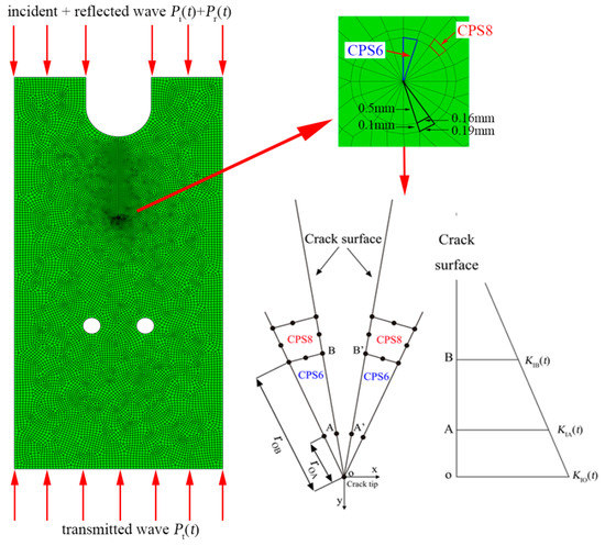
Figure 13.
Mesh of finite element model established in ABAQUS code.
4.2. Calculation Method of Dynamic SIFs
According to the theory of linear elastic fracture mechanics, the SIF can be expressed by the crack tip displacement with Equation (9):
where E is the elastic modulus, νd is the Poisson’s ratio, k = 3-4νd, u is the displacement, and KI(t) is SIF. According to the displacement extrapolation method, SIF can be expressed by Equation (10):
where rOA and rOB are the distances from the A and B points to the origin O in the singular element of the crack tip.
Freund [42] proposed that DSIF in the dynamic crack propagation is related to the crack propagation speed and DSIF of the stationary crack with the corresponding crack length. The relation can be expressed by Equation (11):
where KId(t) is the DSIF of crack with a certain speed, v is crack propagation speed, KI0(t) is the DSIF of the stationary crack with corresponding crack length, k(v) is the universal function, as shown by Equation (12):
where cR is Rayleigh wave velocity, cD is longitudinal wave velocity.
Figure 14 demonstrates the determination method of the propagation of DSIF. As the curve of dynamic SIF versus time at the crack tip has been obtained by calculation results from ABAQUS, the critical DSIF is determined by the fracture time recorded from the crack propagation gauge in the experiment. Then, the determined KI0(t) and the corresponding velocity is substituted into Equations (11) and (12), and the propagation DSIF, KId(t), can be acquired.
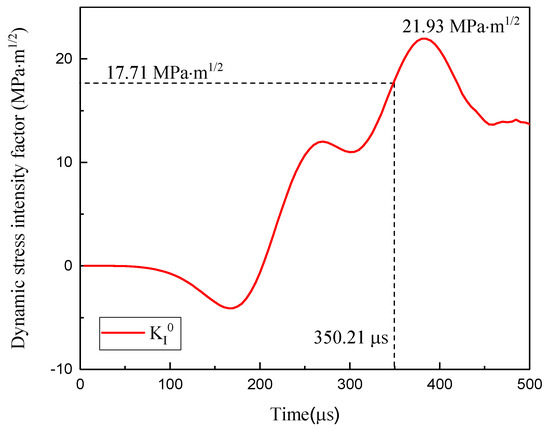
Figure 14.
The curve of dynamic stress intensity factor (SIF) versus time and determination method of propagation dynamic stress intensity factor (DSIF).
Therefore, according to the method discussed above, the crack propagation DSIF in the complete process with three loading rates were calculated, as shown in Figure 15. It is clear that the crack initiation DSIF is the highest among the whole crack propagation process. During the crack propagation process, the DSIF has a decreasing trend after initiation. However, when running crack is arrested with very low velocity, the arrest DSIF, which is a particular kind of propagation DSIF, increased significantly.

Figure 15.
Crack propagation dynamic stress intensity factor in the complete process.
Taking the effect of the loading rate into consideration, although the three DSIF curves have a consistent trend, the crack propagation DSIF has an entire enlargement as the loading rate rises. Especially when the loading rate rises from 1500 GPa·s−1 to 2000 GPa·s−1, the amplification of DSIF is more pronounced than the one from 1000 GPa·s−1 to 1500 GPa·s−1. Under loading rate 1000 GPa·s−1, the initiation DSIF is 12.21 MPa·m1/2, the minimum propagation DSIF is 5.25 MPa·m1/2, and arrest DSIF is 8.39 MPa·m1/2. Under loading rate 1500 GPa·s−1, the initiation DSIF is 16.41MPa·m1/2, the minimum propagation DSIF is 8.00 MPa·m1/2, and arrest DSIF is 12.57 MPa·m1/2. Under loading rate 2000 GPa·s−1, the initiation DSIF is 19.42 MPa·m1/2, the minimum propagation DSIF is 11.3 MPa·m1/2, and arrest DSIF is 16.20 MPa·m1/2. All the above shows that loading rate does have a significant effect on crack propagation DSIF.
5. Conclusions
In this paper, an experimental investigation combining SHPB and numerical simulation study was applied to understand the dynamic propagation behaviour and crucial mechanical parameters of crack propagation in the complete process. Several conclusions have been achieved, as follows:
- The crack arrest position is predictable in ISCSC specimens, which can be applied in investigating dynamic crack propagation behavior and measuring crack propagation DSIF in a complete process.
- The symmetrical holes have a significant effect on the crack propagation behavior and the extrusion caused by their deformation seriously restricts the propagation of the main crack.
- The crack propagation velocity increases with the loading rate, and the effect of the symmetrical holes on a propagating crack is magnified by the increase in loading rate.
- The arrest DSIF is larger than average propagation DSIF, but smaller than initiation DSIF. The crack propagation DSIF in the whole process has an entire increase with the rising loading rate.
Author Contributions
Conceptualization, F.W., M.M.N. and M.W.; methodology, F.W. and M.W.; software, F.W. and P.Y.; validation, F.W. and M.W.; formal analysis, F.W.; investigation, F.W.; resources, F.W. and H.Q.; data curation, F.W. and C.N.; writing—original draft preparation, F.W.; writing—review and editing, F.W., M.W. and M.M.N.; visualization, F.W. and M.W.; supervision, M.W.; funding acquisition, M.W. and M.M.N.
Funding
This research was funded by the National Natural Science Foundation of China (grant numbers 11702181), the China Postdoctoral Science Foundation (grant number 2016M602689), the Fundamental Research Funds for the Central Universities (grant number 2018SCU12047) and China Scholarship Council (grant number 201806245024).
Conflicts of Interest
The authors declared that they have no conflicts of interest in this work. And we declare that we do not have any commercial or associative interest that represents a conflict of interest in connection with the work submitted.
References
- Zhang, X.P.; Wong, L.N.Y. Cracking Processes in Rock-Like Material Containing a Single Flaw Under Uniaxial Compression: A Numerical Study Based on Parallel Bonded-Particle Model Approach. Rock Mech. Rock Eng. 2012, 45, 711–737. [Google Scholar] [CrossRef]
- Nezhad, M.M.; Fisher, Q.J.; Gironacci, E.; Rezania, M. Experimental Study and Numerical Modeling of Fracture Propagation in Shale Rocks During Brazilian Disk Test. Rock Mech. Rock Eng. 2018, 51, 1755–1775. [Google Scholar] [CrossRef]
- Gironacci, E.; Nezhad, M.M.; Rezania, M.; Lancioni, G. A non-local probabilistic method for modeling of crack propagation. Int. J. Mech. Sci. 2018, 144, 897–908. [Google Scholar] [CrossRef]
- Nezhad, M.M.; Gironacci, E.; Rezania, M.; Khalili, N. Stochastic modelling of crack propagation in materials with random properties using isometric mapping for dimensionality reduction of nonlinear data sets. Int. J. Numer. Methods Eng. 2017, 113, 656–680. [Google Scholar] [CrossRef]
- Shao, J.F.; Zhu, Q.Z.; Su, K. Modeling of creep in rock materials in terms of material degradation. Comput. Geotech. 2003, 30, 549–555. [Google Scholar] [CrossRef]
- Banadaki, M.M.D.; Mohanty, B. Numerical simulation of stress wave induced fractures in rock. Int. J. Impact Eng. 2012, 40, 16–25. [Google Scholar] [CrossRef]
- Alam, M.; Grimm, B.; Parmigiani, J.P. Effect of incident angle on crack propagation at interfaces. Eng. Fract. Mech. 2016, 162, 155–163. [Google Scholar] [CrossRef]
- Bleyer, J.; Rouxlanglois, C.; Molinari, J.F. Dynamic crack propagation with a variational phase-field model: Limiting speed, crack branching and velocity-toughening mechanisms. Int. J. Fract. 2017, 204, 79–100. [Google Scholar] [CrossRef]
- Carpiuc-Prisacari, A.; Poncelet, M.; Kazymyrenko, K.; Leclerc, H.; Hild, F. A complex mixed-mode crack propagation test performed with a 6-axis testing machine and full-field measurements. Eng. Fract. Mech. 2017, 176, 1–22. [Google Scholar] [CrossRef]
- Wang, X.; Zhu, Z.; Meng, W.; Peng, Y.; Lei, Z.; Dong, Y. Study of rock dynamic fracture toughness by using VB-SCSC specimens under medium-low speed impacts. Eng. Fract. Mech. 2017, 181, 52–64. [Google Scholar] [CrossRef]
- Haeri, H.; Shahriar, K.; Marji, M.F.; Moarefvand, P. Experimental and numerical study of crack propagation and coalescence in pre-cracked rock-like disks. Int. J. Rock Mech. Min. Sci. 2014, 67, 20–28. [Google Scholar] [CrossRef]
- Zhang, C.W.; Gholipour, G.; Mousavi, A.A. Nonlinear dynamic behavior of simply-supported RC beams subjected to combined impact-blast loading. Eng. Struct. 2019, 181, 124–142. [Google Scholar] [CrossRef]
- Gao, D.W.; Zhang, C.W. Theoretical and numerical investigation on in-plane impact performance of chiral honeycomb core structure. J. Struct. Integr. Maint. 2018, 3, 95–105. [Google Scholar] [CrossRef]
- Chong, K.P.; Kuruppu, M.D. New specimen for fracture toughness determination for rock and other materials. Int. J. Fract. 1984, 26, R59–R62. [Google Scholar] [CrossRef]
- Aliha, M.R.M.; Ayatollahi, M.R. Mixed mode I/II brittle fracture evaluation of marble using SCB specimen. Procedia Eng. 2011, 10, 311–318. [Google Scholar] [CrossRef]
- Grégoire, D.; Maigre, H.; Réthoré, J.; Combescure, A. Dynamic crack propagation under mixed-mode loading—Comparison between experiments and X-FEM simulations. Int. J. Solids Struct. 2007, 44, 6517–6534. [Google Scholar] [CrossRef]
- Wang, M.; Zhu, Z.; Dong, Y.; Lei, Z. Study of mixed-mode I/II fractures using single cleavage semicircle compression specimens under impacting loads. Eng. Fract. Mech. 2017, 177, 33–44. [Google Scholar] [CrossRef]
- Ravi-Chandar, K.; Knauss, W.G. An experimental investigation into dynamic fracture: I. Crack initiation and arrest. Int. J. Fract. 1984, 25, 247–262. [Google Scholar] [CrossRef]
- Eberhardt, E.; Stead, D.; Stimpson, B.; Read, R.S. Identifying crack initiation and propagation thresholds in brittle rock. Can. Geotech. J. 1998, 35, 222–233. [Google Scholar] [CrossRef]
- David, G.; Hubert, M.; Alain, C. New experimental and numerical techniques to study the arrest and the restart of a crack under impact in transparent materials. Int. J. Solids Struct. 2009, 46, 3480–3491. [Google Scholar]
- Gao, G.; Yao, W.; Xia, K.; Li, Z. Investigation of the rate dependence of fracture propagation in rocks using digital image correlation (DIC) method. Eng. Fract. Mech. 2015, 138, 146–155. [Google Scholar] [CrossRef]
- Chen, R.; Xia, K.; Dai, F.; Lu, F.; Luo, S.N. Determination of dynamic fracture parameters using a semi-circular bend technique in split Hopkinson pressure bar testing. Eng. Fract. Mech. 2009, 76, 1268–1276. [Google Scholar] [CrossRef]
- Yang, R.; Peng, X.; Yue, Z.; Cheng, C. Dynamic fracture analysis of crack–defect interaction for mode I running crack using digital dynamic caustics method. Eng. Fract. Mech. 2016, 161, 63–75. [Google Scholar] [CrossRef]
- Estevez, R.; Tijssens, M.G.A.; Giessen, E.V.D. Modeling of the competition between shear yielding and crazing in glassy polymers. J. Mech. Phys. Solids 2000, 48, 2585–2617. [Google Scholar] [CrossRef]
- Marsavina, L.; Sadowski, T.; Knec, M. Crack propagation paths in four point bend Aluminium–PMMA specimens. Eng. Fract. Mech. 2013, 108, 139–151. [Google Scholar] [CrossRef]
- Saksala, T.; Hokka, M.; Kuokkala, V.T.; Mäkinen, J. Numerical modeling and experimentation of dynamic Brazilian disc test on Kuru granite. Int. J. Rock Mech. Min. Sci. 2013, 59, 128–138. [Google Scholar] [CrossRef]
- Zhu, Z. Numerical prediction of crater blasting and bench blasting. Int. J. Rock Mech. Min. Sci. 2009, 46, 1088–1096. [Google Scholar] [CrossRef]
- Zhu, Z.; Mohanty, B.; Xie, H. Numerical investigation of blasting-induced crack initiation and propagation in rocks. Int. J. Rock Mech. Min. Sci. 2007, 44, 412–424. [Google Scholar] [CrossRef]
- Zhu, Z.; Chao, W.; Kang, J.; Li, Y.; Meng, W. Study on the mechanism of zonal disintegration around an excavation. Int. J. Rock Mech. Min. Sci. 2014, 67, 88–95. [Google Scholar] [CrossRef]
- Zhu, Z.; Xie, H.; Mohanty, B. Numerical investigation of blasting-induced damage in cylindrical rocks. Int. J. Rock Mech. Min. Sci. 2008, 45, 111–121. [Google Scholar] [CrossRef]
- Wang, M.; Wang, F.; Zhu, Z.; Dong, Y.; Mousavi Nezhad, M.; Zhou, L. Modelling of crack propagation in rocks under SHPB impacts using a damage method. Fatigue Fract. Eng. Mater. Struct. 2019, 42, 1699–1710. [Google Scholar] [CrossRef]
- Zhou, L.; Zhu, Z.M.; Dong, Y.Q.; Fan, Y.; Zhou, Q.; Deng, S. The influence of impacting orientations on the failure modes of cracked tunnel. Int. J. Impact Eng. 2019, 125, 134–142. [Google Scholar] [CrossRef]
- Eringen, A.C.; Suhubi, E.S.; Chao, C.C. Elastodynamics, Vol. II, Linear Theory. J. Appl. Mech. 1978, 45, 229. [Google Scholar] [CrossRef][Green Version]
- Zhang, Q.B.; Zhao, J. A Review of Dynamic Experimental Techniques and Mechanical Behaviour of Rock Materials. Rock Mech. Rock Eng. 2014, 47, 1411–1478. [Google Scholar] [CrossRef]
- Wang, Q.Z.; Yang, J.R.; Zhang, C.G.; Zhou, Y.; Li, L.; Wu, L.Z.; Huang, R.Q. Determination of Dynamic Crack Initiation and Propagation Toughness of a Rock Using a Hybrid Experimental-Numerical Approach. J. Eng. Mech. 2016, 142, 9. [Google Scholar] [CrossRef]
- Dong, Y.Q.; Zhu, Z.M.; Zhou, L.; Ying, P.; Wang, M. Study of mode I crack dynamic propagation behaviour and rock dynamic fracture toughness by using SCT specimens. Fatigue Fract. Eng. Mater. Struct. 2018, 41, 1810–1822. [Google Scholar] [CrossRef]
- Lang, L.; Zhu, Z.M.; Zhang, X.S.; Qiu, H.; Zhou, C.L. Investigation of crack dynamic parameters and crack arresting technique in concrete under impacts. Constr. Build. Mater. 2019, 199, 321–334. [Google Scholar] [CrossRef]
- Shao, J.C.; Xiao, B.L.; Wang, Q.Z.; Ma, Z.Y.; Yang, K. An enhanced FEM model for particle size dependent flow strengthening and interface damage in particle reinforced metal matrix composites. Compos. Sci. Technol. 2011, 71, 39–45. [Google Scholar] [CrossRef]
- Bedon, C.; Santarsiero, M. Laminated glass beams with thick embedded connections—Numerical analysis of full-scale specimens during cracking regime. Compos. Struct. 2018, 195, 308–324. [Google Scholar] [CrossRef]
- Li, H.; Fu, M.W.; Lu, J.; Yang, H. Ductile fracture: Experiments and computations. Int. J. Plast. 2011, 27, 147–180. [Google Scholar] [CrossRef]
- Chen, Y.M. Numerical computation of dynamic stress intensity factors by a Lagrangian finite-difference method (the HEMP code) for cracked bars. Eng. Fract. Mech. 1975, 7, 653–660. [Google Scholar] [CrossRef]
- Tikalsky, P.J. Dynamic Fracture Mechanics; By L.B. Freund; Cambridge University Press: New York, NY, USA, 1990; p. 563. [Google Scholar]
© 2019 by the authors. Licensee MDPI, Basel, Switzerland. This article is an open access article distributed under the terms and conditions of the Creative Commons Attribution (CC BY) license (http://creativecommons.org/licenses/by/4.0/).