Abstract
We present a comparative study between predictive monthly rainfall models for islands of complex orography using machine learning techniques. The models have been developed for the island of Tenerife (Canary Islands). Weather forecasting is influenced both by the local geographic characteristics as well as by the time horizon comprised. Accuracy of mid-term rainfall prediction on islands with complex orography is generally low when carried out with atmospheric models. Predictive models based on algorithms such as Random Forest or Extreme Gradient Boosting among others were analyzed. The predictors used in the models include weather predictors measured in two main meteorological stations, reanalysis predictors from the National Oceanic and Atmospheric Administration, and the global predictor North Atlantic Oscillation, all of them obtained over a period of time of more than four decades. When comparing the proposed models, we evaluated accuracy, kappa and interpretability of the model obtained, as well as the relevance of the predictors used. The results show that global predictors such as the North Atlantic Oscillation Index (NAO) have a very low influence, while the local Geopotential Height (GPH) predictor is relatively more important. Machine learning prediction models are a relevant proposition for predicting medium-term precipitation in similar geographical regions.
1. Introduction
The weather is one of the main concerns in the Canary Islands, especially in those islands with very abrupt orography. On the one hand, the agricultural sector in the Canary Islands can be described as segmented, very sensitive to rainfall and without permanent watercourses. On the other hand, the main economic activity in the Canary Islands is tourism, which attracts large numbers of floating population. In addition, the wide variety of meteorological factors occurring in the Canary Islands make rainfall prediction an important issue and, together with its temporal estimation, constitutes an essential factor for decision making and to minimize potential risks linked to sudden increases and the considerable disperse distribution of the affected areas.
The Canary Islands are part of the Macaronesia and are located northwest of the Atlantic Ocean reaching from 27°37′ to 29°25′ N and from 13°20′ to 18°10′ W. The Canary Islands archipelago is made up of eight main islands lined from East to West and ten smaller isles (Figure 1).

Figure 1.
Canary Islands, National Aeronautics and Space Administration (NASA) image acquired 13 October 2011.
The island of Tenerife, with a population close to 900,000 inhabitants and the annual visit of more than six million tourists, is the most populated island and the largest in the archipelago. In fact, it is one of the areas with the highest population density in Europe (440 inhabitants/km2).
The island, located approximately 300 km west of the northern coast of Africa, is characterized by an uneven and steep orography with sharp slopes from the inner part to the coast. The central area is crowned by a mountain range with Teide volcano on top (3718 m), which divides the island into two highly differentiated climatic areas: the southern and the northern area. The southern area is drier because the mountains block the passage of trade winds and the northern area is relatively wetter precisely because of the effect of those trade winds. Overall precipitation is low [1], with an annual average of 233 mm on the whole island. Distribution of rainfall is heterogeneous, with a large percentage of rainfall occurring in short periods of time and sparse in space. These factors mean that sudden increases in rainfall constitute a serious issue that has led to the loss of human lives as well as economic loss in sectors such as tourism, agriculture, and communications infrastructure. Therefore, weather forecasting and climate analysis are lines of research that are prioritized.
In this paper, we develop and compare several rainfall prediction models using machine learning techniques (ML) for the island of Tenerife resulting in a classification of rainy or dry months. In order to do this, we used a meteorological dataset [2] for a period of time of 41 years of registered data, from 1976 to 2016.
2. Literature Review
Most research works on weather prediction are carried out through numerical methods. These methods are carried out by using the laws of fluid dynamics and of chemical processes taking place in the atmosphere to then integrate all the meteorological data available onto a computational grid and project their evolution in time. There are two types of models according to the resolution of their computational grid: synoptic scale models (macro-scale with wide mesh of 40 km or wider) and regional scale models (mesoscale with meshes of a few kilometers), which have better spatial and temporal resolution. There are many models being used nowadays, both government and private models. For instance, the Global Forecast System (GFS) model [3] is a numerical weather prediction model produced by the National Center for Environmental Prediction-National Oceanic and Atmospheric Administration (NOAA-NCEP). GFS is an open and free model at a synoptic scale with horizontal resolution of 27 km for mid-term prediction (eight days) and resolution of 70 km for long-term prediction (16 days). There is also the Weather Research and Forecasting (WRF) model [4], which is a mesoscale system limited to a specific region (between 2 and 15 km) and mid-term weather prediction (1–2 days), and thus closer to reality. Another model is the European Centre for Medium-Range Weather Forecasts (ECMWF) model [5], a system with horizontal resolution of 9 km for 10-day prediction and a resolution of 18 km for 15 days. On the one hand, one of the main problems of weather forecasting with numerical methods is their poor performance in segmented regions with abrupt orography, which make them not very suitable for the prediction of the evolution of Mesoscale Convective Systems (MCS). On the other hand, there are numerous contributions regarding the use of ML models for weather prediction, despite the permanent controversy that, although through ML we can obtain models to predict a meteorological phenomenon in a more or less reliable way, ML cannot explain these phenomena in physical terms.
In the reviewed literature, most research in meteorological prediction has been carried out mainly in two areas: the construction of models based on machine learning for the prediction of meteorological parameters in general and specific models for rainfall prediction, these ones due to the need to estimate risks appropriately and also because of economic reasons. With regard to the first models mentioned, it is worth highlighting the works of [6,7,8,9,10]. In [10], several data mining algorithms (DM) are explored using large datasets, especially daily meteorological data from NOAA, which make it possible to identify climate patterns and make valid mid-term predictions. In addition, in [8], useful knowledge is extracted from a 9-year period of meteorological data using DM. The steps taken in this study are: data preprocessing, outlier analysis, clustering, classification, and prediction. Each technique used is classified according to its relevance in the prediction. A more specific application is proposed in [7], where authors use a model to show the relationship between meteorological parameters read in meteorological stations and secondary parameters such as vertical velocity variance or surface heat flux. In the study by [9], a hybrid global climate model is suggested (HGCM) through the use of neural networks to speed up the calculations of predictions. In the work by [6], the authors suggest a procedure to predict the behavior of chaotic systems. As an application, this technique is used to obtain stable behavioral patterns of the North Atlantic Oscillation (NAO) index in its prediction through independent component analysis for spatiotemporal data of the variable sea-level pressure (SLP). Calculations are validated with temporal data registered by the NAO index.
Among the literature reviewed, there are other specific models that range from models for the prediction of the number of solar irradiance hours in a specific geographic area [11], to models for the prediction of wind gusts for agriculture applications [12], or even models for the classification of the quality of wine in a specific region depending on meteorology [13]. In the study by [11], several ML methods are presented to obtain predictions of solar radiation through an analysis to compare the different margins of error in predictions. In order to improve the characteristics of the predicting algorithm, a series of hybrid models or ensemble models used by different authors are presented. In the paper by [12], authors study wind gust prediction. This forecasting is characterized by the high variability and brief duration of wind gusts and because they occur suddenly and end abruptly. This work suggests a pattern based on the application of ML techniques, which classifies those gusts by using thousands of measurements made using both real-time variables and variables from mathematical models. Finally, in [13], authors developed an application using DM techniques to predict wine quality depending on climatic, physical, and crop yield factors. In order to do so, an artificial neural network algorithm was used to classify the data associations and the chi-square test was used to establish the degree of dependence between the related variable values.
In [14], the authors propose the integration of meteorological data from different sources of the so-called Data Mining Meteo (SMM) system, which makes it possible to obtain, by using DM techniques, quick predictions, even in the presence of randomly occurring changing phenomena. The applications focus on the short-term prediction of meteorological events such as fog and low cloud cover. Furthermore, in [15], the authors make cloud-ceiling-height forecast based on METAR meteorological data at JFK airport. In this work, the authors conclude that ML algorithms show better prediction results than methods based on Numerical Weather Prediction (NWP) models. In a different study [16], the authors propose an interesting multimodal algorithm for predicting visibility due to atmospheric conditions, not only related to meteorological variables, but also taking into account pollution from gaseous effluent contamination of factory exhaust in a given area. For this purpose, an advanced numerical prediction model and a method for detecting gaseous pollutant emissions are used. Two numerical regression algorithms, the XGBoost and the LightGBM, are used to train the prediction model, to which the estimation data based on Landsat-8 satellite images are added to help in the prediction. The results obtained by this numerical prediction model are more accurate than those obtained by other methods.
In [17], the authors introduce a system to obtain accurate short-term predictions, which uses regression functions and data collected from weather stations, including temperature, wind speed, solar radiation and pressure, humidity, cloudiness, and rainfall. After preprocessing these data, the prediction results obtained are compared with SVM, regression tree (RF), and a fit linear model (FITLM). The results show the robustness of the system.
In [18], the authors propose the use of a modified algorithm based on XGBoost for forecasting wind energy for use in the electrical system. The results of this model are compared with others, based on neural networks (BPNN), regression trees (CART), support vector regression (SVR), and, with a simple XGBoost model, obtaining the best accuracy results in the prediction.
The rainfall estimation models suggested use either numerical historical data from meteorological stations or data from reanalysis software or from these combined with images. Among the first type, it is worth highlighting the model proposed in [19], which proposes a DM algorithm for rainfall prediction over the monsoon period in the Indian peninsula combined with statistical techniques and which predicts rainfall in five categories. In [20], the authors compare the predictive characteristics with Markov Chains with extended rainfall prediction and six other ML algorithms and find very good results, which even allow for detecting correlations between different climates and their predictive accuracy. Models including image processing use neural networks, like in the model proposed in [21], which focuses on the prediction of rainfall in a local region over a short period of time using ML techniques and working with spatiotemporal datasets. In order to tackle this problem, the authors suggest the use of Recurrent Neural Networks (RNN) with a convolutional structure. This methodology is applied in rainfall prediction systems based on radar image analysis of rainfall over a certain period. In addition, in [22], the authors develop an approach based on spatial analysis with DM techniques to enable the deduction of the correlations and causalities between satellite images of the moving trajectories of Mesoscale Convective Systems (MCS) and heavy rainfall in Tibet. The proposed approach proves to be efficient by automatically analyzing large meteorological datasets to assist weather forecasting.
In [23], a machine learning method algorithm based on support vector machine with dislocation of temporal variables (DSVM) was used to make short-term rain predictions.
For this purpose, data from meteorological stations and satellite meteorological images were used. The results were validated using weather threat scores, showing good forecasts within 1 to 6 h.
In [24], the authors present a new approach for predicting rainfall and runoff in river basins over the next two months. To do this, the authors propose a combination of wavelet transform and artificial neural network (WANN) that incorporates observed and predicted time series in the input structure. The comparison between the performance of the proposed WANN model and the performance of traditional WANN models through an uncertainty analysis reveals the superiority of the model proposed in this study.
Finally, in [25], a machine learning algorithm based on random forest (RF) is used to make quantitative estimates of rainfall. Satellite temperature data are combined with numerical weather prediction (NWP) data from the global forecast system. In general, this algorithm obtains better predictive results over ocean surfaces, underestimating the prediction of the rainfall rate over land. However, the selected RF classification model allows the precipitation area to be predicted with an accuracy of 0.87.
In recent years, research has intensified in the analysis of weather prediction models, specifically of rainfall, both in the medium term and in the short term, using various techniques of Machine learning and Deep Learning [26,27,28,29]. There exists a notable trend in the experimentation of models based on neural networks. However, these models require a careful selection and preprocessing of the weather predictors chosen to fit the physical environment in which the study is conducted.
This paper proposes an analytic solution based on machine learning techniques, which allows monthly rainfall prediction. The data used include mainly meteorological datasets available from meteorological stations of the island of Tenerife and reanalysis values from NOAA databases.
Climate in the Canary Islands
Some of the climatic characteristics of the Canary Islands have been thoroughly studied by several authors [30,31,32]. The average trade winds blow mainly against the north side of the islands, and these rise over the island slopes due to the orography leading to condensation and cloud growth resulting in three layers: (1) a layer of fresh and moist air at low levels, (2) a subsidence inversion layer with temperature increase, and (3) a layer of dry and clear air at high levels. However, the movement of these winds below 1000 m is very affected by the abrupt orography such as small valleys, forests, cliffs, etc., which lead and channel the winds at lower levels (Figure 2).
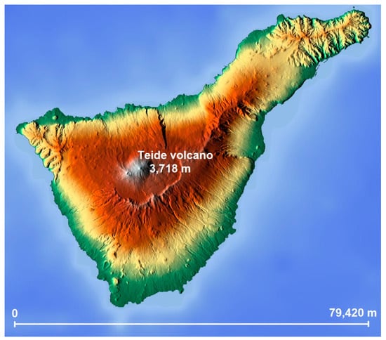
Figure 2.
Orographic model of the Tenerife Island (Google Maps).
The most significant precipitation occurs when disturbances break the inversion layer that are associated with low pressure or due to disturbances in upper levels (troughs), which cannot be detected at the surface level and are only evident when upper layers are analyzed [31].
The latter are the disturbances causing rainfall in the oriental islands with lower orography, but these also significantly affect the rest of the islands in the archipelago.
Despite all of the above, according to several authors, the climate in the Canary Islands is generally stable with a high signal-to-noise ratio in meteorological observations [30], which is why it is relatively easy to determine an actual “trend” over time as the background fluctuations do not vary significantly. Nevertheless, other authors consider that these relatively low precipitation rates, on the contrary, introduce higher noise in the time series of rainfall measurement [33], which makes their study more complicated.
This is one of the aspects that has led to the use of climatic studies based on statistical techniques [34] as long as a complete meteorological database is used.
Although the relief is the main factor that affects the local rainfall distribution [31], the combination of the above-mentioned factors makes rainfall prediction difficult at the local level. A temporal analysis of the rainfall distribution on the island of Tenerife shows that it is not homogeneous over the period of time analyzed (1976 to 2016). However, certain seasonality is observed over the months from January to March and from October to December. High precipitation rates are observed over certain periods, which do not always coincide with the traditionally rainier months of the year (Figure 3).
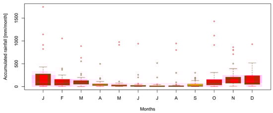
Figure 3.
The graphic shows asymmetric precipitation distribution and outliers. Monthly rainfall of forty-one years on the island of Tenerife (1976 to 2016). The non-rainy months are in orange and the rainy ones are in red.
In the present work, global and local meteorological parameters are used for the development of a predictive model. Global parameters are associated with precipitation and meteorological phenomena occurring in the archipelago on average, an issue which has been already studied by other authors. For instance, in [35], the authors relate the NAO index and heavy rainfall in the winter season in Spain; in [31], the authors highlight the importance of predicting global parameters and their relationship with rainfall in the Canary Islands and use it to characterize precipitation rates in the archipelago, and, in [34], to predict the intensity of monsoon rains in India.
We obtained local parameters from measurements of meteorological stations and from reanalysis of databases from NOAA (NCEP/NCAR Reanalysis). In this study, we worked with the following parameters for the development of a rainfall predictive model in the island of Tenerife. On the one hand, NAO global parameter and local reanalysis parameters: (1) Sea Level Pressure (SLP); (2) Sea Surface Temperature (SST) and (3) geopotential height 500-hPa (GPH). On the other hand, local parameters from meteorological stations: (1) monthly accumulated rainfall and monthly measurements of (2) temperature, (3) wind speed, (4) pressure, and (5) relative humidity. More information on the units of the meteorological parameters can be found in Appendix A. For the island of Tenerife, two meteorological stations were selected from the ones available (Figure 4): Santa Cruz de Tenerife meteorological station (C449C) and the meteorological station at Tenerife North Airport (C447A) (Table 1).
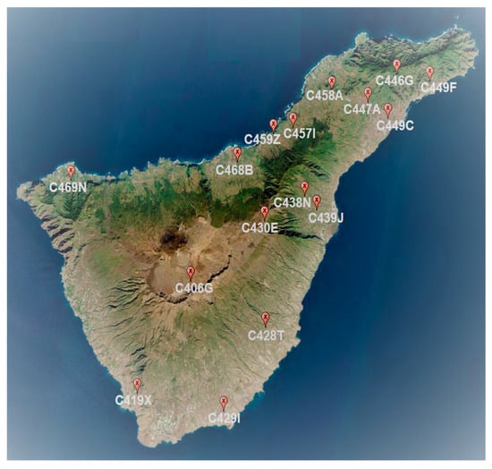
Figure 4.
Main weather stations on Tenerife island (Grafcan).

Table 1.
Main weather stations on Tenerife Island. The asterisk * identifies the selected Tenerife North Airport and Santa Cruz de Tenerife weather stations.
The main reason for using data from only these two meteorological stations is that they are the only ones with 41 years of continuous data. Despite their proximity, both stations are a good example of the island’s dry and humid climates, due to the island’s complicated orography.
In addition, the station (C449C) is located in the most populated city on the island and contains its main port with the largest number of tourist cruises. The station (C447A) is only 10 km away from the previous one, but with a difference in height of about 600 meters and oriented to the trade winds that give it completely different climatic characteristics.
3. Materials and Methods
This section describes the methodology and data used in the experiments and also includes a brief description of the machine learning algorithms used in the determination of the prediction models.
There exist several methods for analytical processes among which the most popular methodologies are a Cross-Industry Standard Process for Data Mining (CRISP-DM) [36] and Sample, Explore, Model, and Assess (SEMMA) [37]. CRISP-DM and SEMMA are similar although they differ in the definition of the stages and the number of stages [37]. Our proposal consists of the following phases that result in an acceptable predictive model: (1) training (apply a machine learning algorithm to the training data set so that the model learns), (2) validation (estimate the error of a predictive model with unseen data), (3) hyperparameters (there is no way to know beforehand which parameters of the algorithm throw the best model, and it is therefore necessary to apply validation strategies), and (4) prediction (once the model is obtained, it is used to predict new observations). Figure 5 presents a flowchart of the proposed method.
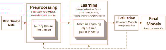
Figure 5.
General flowchart of the proposed method.
3.1. Model and Data Acquisition
The reason behind the development of a monthly predictive model is the importance, from an economic point of view, of the evaluation of short-term precipitation trends (monthly periods). The presence of effective data sources is essential in the development of a rainfall predictive model. The elaboration of the model has been decided over the analysis of monthly accumulated rainfall data [2], which shows some seasonality and high concentration of low precipitation values.
The response or class variable depends on the maximum monthly accumulated rainfall registered in both stations (C447A and C449C) over a period of time of 41 years (1976 to 2016). The accumulated rainfall registered determines whether a month is wet or dry, thus creating a binary classification predictive model (dry or wet).
The group of predictors for the development of the model consists of local variables from the meteorological stations, reanalysis variables available on a 2.5° 3 × 2 grid from 29.5 N to 18.5 W and 27.5 N to 13.5 W, covering the whole Canary Islands archipelago- and the NAO index. Local variables have been taken from the NOAA database, using the R software package, stationary [38] and RNCEP [39].
Among the classification problems, an imbalance in the frequencies of the observed classes can have a significant negative impact on the effectiveness of the model [40,41,42]. A data set is imbalanced if the classification categories are not approximately equally represented [43,44]. A possible remedy to solve such class imbalance is to resample the training data in a way that mitigates these problems [43].
Finding the best model is not a trivial issue; there are many (several tens) of algorithms, each one of them with their own characteristics and with different parameters that need to be adjusted [45,46,47].
In the model training, validation and search for hyperparameters, several metrics are used that allow for assessing the quality of the machine learning algorithm in its predictions. The optimal metric depends entirely on the problem to be solved. In the present work, months are classified into the categories of rainy or non-rainy months. Accuracy and kappa metrics are among the most popular used in binary and multiclass classification problems. Accuracy allows us to assess the percentage of observations correctly classified with respect to the total of predictions, and kappa is the normalized accuracy value with respect to the percentage of hits expected [48,49,50].
3.2. Algorithms and Frameworks
In this paper, several algorithms were examined for goodness of fit.
Random forest (rf) is an aggregation technique suggested in [51] and considered one of the most precise general purpose tools. It consists of the creation of several decision trees over samples of a data set generated by random sampling with replacement. Its basic principle consists of injecting randomness to the construction of each individual tree to improve accuracy of the aggregated model.
Linear Discriminant Analysis (lda) [52] is a linear transformation technique used to reduce dimensionality. lda determines the directions (linear discriminants) representing the axes that maximize the separation between multiple classes.
Logistic Model Trees (lmt) combine model trees and logistic regression functions at the leaves. A stagewise fitting process is used to construct the logistic regression models that can select relevant attributes in the data [53].
Generalized Linear Model (glm) is a generalization of classic linear regression. Generalized linear models were presented [54] in 1998 as a way of unifying several other statistical models including linear regression, logistic regression, and Poisson regression under one theoretical framework. This allowed them to develop a general algorithm to estimate maximum likelihood in all these models.
In 1992, Vapnik [55] presented support vector machines (svm), a specific class of algorithms characterized by the usage of kernels, absence of local minima, and control over the number of supporting vectors. Support vector machines can be applied both to classification and regression problems [56].
Friedman [57,58] presented the Stochastic Gradient Boosting (gbm) algorithm. This algorithm employs several models that aggregate and result in a final model with better predictive accuracy than that of the models used individually.
The eXtreme Gradient Boosting (XGBoost) software library is an open source implementation of a supervised learning algorithm that attempts to predict in an appropriate way a destination variable by combining estimations of a group of simpler and weaker models. It offers several advanced features for model tuning, computing environments, and algorithm enhancement [59]. XGBoost is suitable for performing the three main forms of gradient boosting, and it is robust enough to support fine-tuning and inclusion of regularization parameters. XGBoost has proven to work quite well in automatic learning competitions.
Nowadays, several frameworks are used to work with predictive models such as CORElearn [60], mlr [61], or Scikit-learn [62]. In the present work, we used the caret package (Classification and Regression Training) [63]. Caret is an interface that unifies under just one framework several machine learning packages, making data preprocessing, training, optimization, and validation of predictive models easier, and with native support for parallel calculations [43].
3.3. Experiments
The experiments were carried out using the methodology presented and the meteorological data selected. The reanalysis local variables of the grid are averaged monthly, as well as the variables measured in meteorological stations and the NAO index (Table 2). Initial predictors for the construction of the model totals for 12 predicting variables and one response or class variable, with a total of 492 instances corresponding to the months between the years comprised (1976–2016) [2]. The process to prepare the data for the construction of a machine learning predictive model consisted of three steps: selection, preprocessing, and transformation. During the preprocessing of the data set, outliers and highly correlated predictors were identified and removed. It is very important to observe how the attributes relate to each other. An excellent way to analyze interactions between numerical attributes is calculating correlations between each pair. These pair correlations can be plotted in a correlation matrix to give an idea of which attributes change together. Zero deviations show a more positive or negative correlation. Values above 0.75 or below −0.75 are perhaps more interesting, as they show a high positive correlation or a high negative correlation. Values 1 and –1 show a full positive or negative correlation. In the graph, it can be seen that some of the attributes are highly correlated (Figure 6). Outliers and highly correlated in data can distort predictions and affect the accuracy. Clustering of the class variable was obtained with the K-medoids clustering algorithm or PAM (Partitioning Around Medoids), which is less sensitive to outliers compared to k-means [64]. The optimal number of clusters determined was two. The first (Cdry) with in the range of [0 to 125] mm/month of rainfall, and the second (Cwet) with [126 to ∞] mm/month of rainfall.
Table 2.
Shortlisted predictors and their representation.
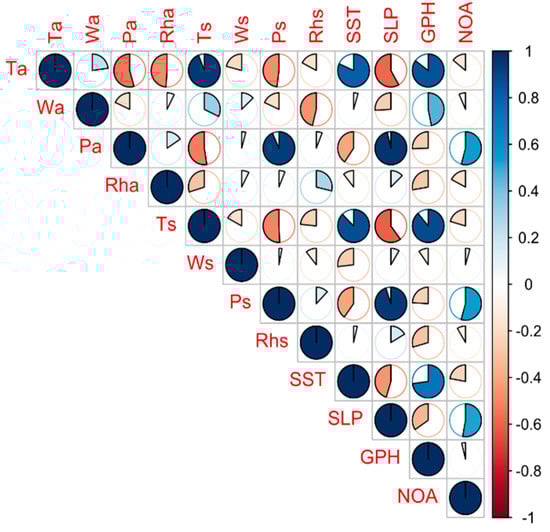
Figure 6.
Identification of highly correlated predictors (conf. level = 0.95). It shows the between-predictor correlations of the transformed continuous predictors; there are many strong positive correlations (indicated by large, dark blue circular sector).
The imbalances in the frequencies of the observed classes (unbalanced classes) were treated to avoid having a negative impact on the predictive models. The random sampling (with replacement) carried out allows the minority class to be the same size as the majority class. Predictors were preprocessed so that they would work with the ML algorithm or improve their results [65]. We selected the cases with 80% proportion for training and with 20% proportion for testing in order to estimate how the model would perform with unseen data. Data preprocessing was learned from the training observation and was later applied to the testing set (e.g., centering and scaling of data were carried out).
The ML algorithms selected allow the construction of a predictive model that is able to represent the patterns present in the training data set and generalize these in new observations (Table 3).
Table 3.
Algorithms applied, training, testing metrics, and level of interpretability.
These algorithms are among the most representative (linear, nonlinear, and ensemble) and their optimal hyperparameters are shown in Table 4. The first step in tuning the model is to choose a set of parameters to evaluate. Once the model and tuning parameter values have been defined, the type of resampling should be also be specified. After resampling, the process produces a profile of performance measures available to guide the user as to which tuning parameter values should be chosen. By default, the caret package automatically chooses the tuning parameters associated with the best value, although different algorithms can be used. In this experiment, we use grid search and random search. Five-fold cross-validation was run. The final predictive models were evaluated with the test data set to estimate the prediction ability of each model (Table 3).
Table 4.
Selected algorithms and optimal hyperparameters of the proposed models (tuning).
Preprocessing, training, optimization, and validation of the predictive models were carried out with Caret package [43,63].
In the following figures (Figure 7, Figure 8 and Figure 9), the variation of the accuracy coefficient can be observed as a function of the different tuning parameters of the three best models: rf, gbm, and XGboost.
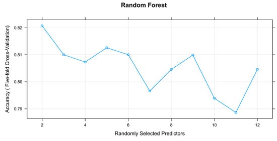
Figure 7.
The accuracy cross-validation profile for a Random Forest model applied the meteorological dataset. The optimal number of predictors is 2.
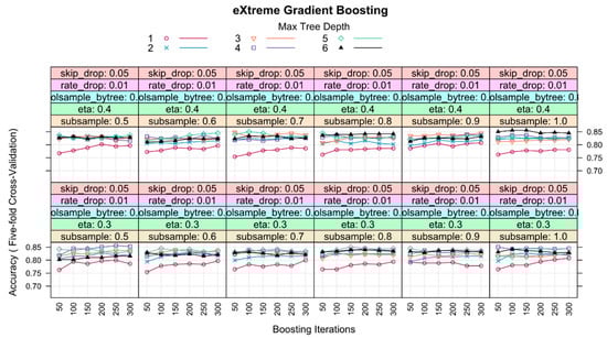
Figure 8.
Accuracy variation by tuning parameter profiles (shows partial view) for the eXtreme Gradient Boosting model using the meteorological dataset [2]. The optimal model used the hyperparameters shown in Table 4.
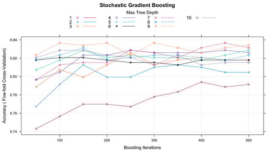
Figure 9.
The cross-validation profiles for a Stochastic Gradient Boosting model applied to the Tenerife meteorological data [2]. The final model was fit using the hyperparameters shown in Table 4.
4. Discussion
In this section, the results obtained in the experiments are shown and discussed. XGBoost and gbm models are the ones providing highest overall accuracy followed closely by rf. Friedman test was performed to determine whether the differences in accuracy were significant. For a significance level α = 0.05 in the Friedman test (p-value = 0.01), evidence was found that the seven classifiers achieve the same accuracy and therefore H0 was rejected. Box and Whisker Plots allow us to observe the spread of the estimated accuracies for different methods and how they are related to each other. The boxes are ordered from highest to lowest mean accuracy. The evaluation metrics are accuracy and kappa because they are easy to interpret. The algorithms were chosen for their diversity of representation and learning style (Figure 10).
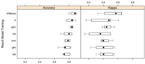
Figure 10.
Results of the model training. A comparison of the cross-validated Accuracy and Kappa estimated from XGBoost (eXtreme Gradient Boosting), rf (Random Forest), gbm (Stochastic Gradient Boosting), lmt (Logistic Model Trees), svm (Support Vector Machine), glm (Generalized Linear Model) and lda (Linear Discriminant Analysis) for meteorological dataset [2].
Cross-validation methods provide good error estimations for a model, although it is valuable to make sure that there is no overfitting. All models (Table 3) achieved more correct predictions in the training set than in the test set, which is why the metrics obtained in training shall not be used as the only option to assess the models since these show an overly optimistic result.
The XGBoost model is the one achieving best results both in the training set and in the testing set. Models based on rf, gbm, and lmt achieve very similar values in the test set. However, according to the contrast of non-parametric Friedman test and the validation results, the models based on lda and glm are inferior to the XGBoost model.
If the priority were to maximize the prediction ability of the model, the XGBoost model would be the best option. However, if interpretability [66] of the model were more important, then the rf or lmt models would be the most suitable.
The most relevant predictors in the XGBoost model are GPH, Rha, Rhs, which contrasts with gbm and rf models. It is worth highlighting that, in the models that provided the highest accuracy (models based on XGBoost, gbm and rf), the NAO predictor is not relevant, which contrasts with the results obtained in other studies carried out in the Canary Islands (Table 5).
Table 5.
Scaled values of the relevance of predictors for gbm, XGBoost, rf, and glm models.
5. Conclusions
In the present work, we have used and compared several already established ML algorithms for monthly rainfall prediction. The performance comparisons and potential applications of learning machines are presented in this paper. This proposal presents very accurate and interpretable predictive models. This research is motivated by the idea of making the process of rainfall prediction simpler and more effective, as well as to overcome the difficulties that other proposals entail. Therefore, the main contributions of this paper are the following: (i) obtaining and comparing rainfall predictive models using several machine learning techniques and (ii) assessing whether the combination of local meteorological variables, NAO index, and the algorithms used has an effect on accuracy of the predictive models. The power of machine learning seems to be an efficient focus for the prediction of meteorological patterns such as rain. The results show that, despite what has been maintained by different authors, in complex orographic geographical areas, global variables such as the North Atlantic Oscillation Index (NAO) have a very low influence on the predictive model obtained, and local variables such as Geopotential Height (GPH) are relatively more important than local variables measured in meteorological stations.
Seasonality predictors have not been applied in the predictive models in order to avoid possible influence on climatology. Machine learning models for rainfall prediction in regions with similar complex orography may also perform excellently. The following aspects will be analyzed in the future. Firstly, long short-term memory (LSTM) networks seem to be suitable for predictions based on time series data, since there can be lags of unknown duration between important events in these series. Secondly, Machine Learning for Streams, through monitoring streaming data from weather stations, is currently one of the most successful applications to forecast data sets in real time. This could be another research line to be explored.
Author Contributions
All the authors have contributed equally to the realization of this work. D.C.-N., R.A.-C., and M.M. participated in the conception and design of the work; D.C.-N., R.A.-C., and M.M. reviewed the bibliography; D.C.-N., R.A.-C., and M.M. conceived and designed the experiments; D.C.-N., R.A.-C., and M.M. performed the experiments; D.C.-N., R.A.-C., and M.M. analyzed the data; D.C.-N., R.A.-C., and M.M. wrote and edited the paper.
Acknowledgments
This work has been possible thanks to the collaboration and support of the University Institute of Intelligent Systems and Numeric Applications in Engineering (IUSIANI-ULPGC).
Conflicts of Interest
The authors declare no conflicts of interest.
Appendix A
This appendix explains and details the equivalences of the units used by some weather predictors in the International System of Units (SI). Table 2, shows the predictors used in this work with their units.
For atmospheric pressures (Ps, Pa, SLP), it is common to obtain data in millibar units, which, according to the IAU (International Astronomical Union), although in continuous use, is obsolete. The SI unit for pressure is the pascal (Pa), equal to one newton per square meter (N/m2).
Equivalence between bar and Pascal:
1 bar = 100,000 Pa = 100,000 N/m2
1 mb = 1 × 10⁻³ bar
1 mb = 1 hPa = 100 Pa
Geopotential height (GPH) is a vertical coordinate referring to the mean level of the Earth’s sea whose units are meters and explains the variation of gravity with latitude and altitude. In meteorology, it is used to express the height at which a given atmospheric pressure (hPa) is found. A geopotential height chart for a single pressure level in the atmosphere shows the troughs and ridges (highs and lows), which can be seen in the weather charts.
References
- Diez-Sierra, J.; del Jesus, M. A rainfall analysis and forecasting tool. Environ. Model. Softw. 2017, 97, 243–258. [Google Scholar] [CrossRef]
- Meteorological Data Set of the Island of Tenerife. Available online: http://dx.doi.org/10.17632/srwzh55hrz.1 (accessed on 1 September 2019).
- Azevedo, A.I.R.L.; Santos, M.F. KDD, SEMMA and CRISP-DM: A Parallel Overview. In Proceedings of the IADIS European Conference Data Mining, Amsterdam, The Netherlands, 24–26 July 2008; pp. 182–185. [Google Scholar]
- Done, J.; Davis, C.A.; Weisman, M. The next generation of NWP: Explicit forecasts of convection using the Weather Research and Forecasting (WRF) model. Atmos. Sci. Lett. 2004, 5, 110–117. [Google Scholar] [CrossRef]
- Trenberth, K.E.; Olson, J.G. An evaluation and intercomparison of global analyses from the National Meteorological Center and the European Centre for Medium Range Weather Forecasts. Bull. Am. Meteorol. Soc. 1988, 69, 1047–1057. [Google Scholar] [CrossRef]
- Basak, J.; Sudarshan, A.; Trivedi, D.; Santhanam, M.S. Weather data mining using independent component analysis. J. Mach. Learn. Res. 2004, 5, 239–253. [Google Scholar]
- Díaz, R.Z.; Montejo, A.M.; Lemus, G.C.; Suárez, A.R. Estimación de parámetros meteorológicos secundarios utilizando técnicas de Minería de Datos. Rev. Cuba. Ing. 2011, 1, 61–65. [Google Scholar]
- Kohail, S.N.; El-Halees, A.M. Implementation of data mining techniques for meteorological data analysis. Int. J. Inf. Commun. Technol. Res. (JICT) 2011, 1, 11–21. [Google Scholar]
- Krasnopolsky, V.M.; Fox-Rabinovitz, M.S. Complex hybrid models combining deterministic and machine learning components for numerical climate modeling and weather prediction. Neural Netw. 2006, 19, 122–134. [Google Scholar] [CrossRef]
- Morreale, P.; Holtz, S.; Goncalves, A. Data Mining and Analysis of Large Scale Time Series Network Data. In Proceedings of the 2013 27th International Conference on Advanced Information Networking and Applications Workshops (WAINA), Barcelona, Spain, 25–28 March 2013; IEEE: Piscataway, NJ, USA, 2013; pp. 39–43. [Google Scholar]
- Voyant, C.; Notton, G.; Kalogirou, S.; Nivet, M.; Paoli, C.; Motte, F.; Fouilloy, A. Machine learning methods for solar radiation forecasting: A review. Renewable Energy 2017, 105, 569–582. [Google Scholar] [CrossRef]
- Sallis, P.J.; Claster, W.; Hernández, S. A machine-learning algorithm for wind gust prediction. Comput. Geosci. 2011, 37, 1337–1344. [Google Scholar] [CrossRef]
- Shanmuganathan, S.; Sallis, P.; Narayanan, A. Data Mining Techniques for Modelling the Influence of Daily Extreme Weather Conditions on Grapevine, Wine Quality and Perennial Crop Yield. In Proceedings of the CICSyN 2010: 2nd International Conference on Computational Intelligence, Communication Systems and Networks, Liverpool, UK, 28–30 July 2010; IEEE: Piscataway, NJ, USA, 2010; pp. 90–95. [Google Scholar]
- Bartok, J.; Habala, O.; Bednar, P.; Gazak, M.; Hluchý, L. Data mining and integration for predicting significant meteorological phenomena. Procedia Comput. Sci. 2010, 1, 37–46. [Google Scholar] [CrossRef]
- Bankert, R.L.; Hadjimichael, M. Data mining numerical model output for single-station cloud-ceiling forecast algorithms. Weather Forecast. 2007, 22, 1123–1131. [Google Scholar] [CrossRef]
- Zhang, C.; Wu, M.; Chen, J.; Chen, K.; Zhang, C.; Xie, C.; Huang, B.; He, Z. Weather Visibility Prediction Based on Multimodal Fusion. IEEE Access 2019, 7, 74776–74786. [Google Scholar] [CrossRef]
- Pérez-Vega, A.; Travieso-González, C.; Hernández-Travieso, J. An Approach for Multiparameter Meteorological Forecasts. Appl. Sci. 2018, 8, 2292. [Google Scholar] [CrossRef]
- Zheng, H.; Wu, Y. A XGBoost Model with Weather Similarity Analysis and Feature Engineering for Short-Term Wind Power Forecasting. Appl. Sci. 2019, 9, 3019. [Google Scholar] [CrossRef]
- Vathsala, H.; Koolagudi, S.G. Long-range prediction of Indian summer monsoon rainfall using data mining and statistical approaches. Theor. Appl. Climatol. 2017, 130, 19–33. [Google Scholar]
- Cramer, S.; Kampouridis, M.; Freitas, A.A.; Alexandridis, A.K. An extensive evaluation of seven machine learning methods for rainfall prediction in weather derivatives. Expert Syst. Appl. 2017, 85, 169–181. [Google Scholar] [CrossRef]
- Shi, X.; Chen, Z.; Wang, H.; Yeung, D.; Wong, W.; Woo, W. Convolutional LSTM network: A machine learning approach for precipitation nowcasting. Adv. Neural Inf. Process. Syst. 2015, 802–810. Available online: http://papers.nips.cc/paper/5955-convolutional-lstm-network-a-machine-learning-approach-for-precipitation-nowcasting (accessed on 1 September 2019).
- Yang, Y.; Lin, H.; Guo, Z.; Jiang, J. A data mining approach for heavy rainfall forecasting based on satellite image sequence analysis. Comput. Geosci. 2007, 33, 20–30. [Google Scholar] [CrossRef]
- Chen, X.; He, G.; Chen, Y.; Zhang, S.; Chen, J.; Qian, J.; Yu, H. Short-term and local rainfall probability prediction based on a dislocation support vector machine model using satellite and in-situ observational data. IEEE Access 2019. [Google Scholar] [CrossRef]
- Alizadeh, M.J.; Kavianpour, M.R.; Kisi, O.; Nourani, V. A new approach for simulating and forecasting the rainfall-runoff process within the next two months. J. Hydrol. 2017, 548, 588–597. [Google Scholar] [CrossRef]
- Min, M.; Bai, C.; Guo, J.; Sun, F.; Liu, C.; Wang, F.; Xu, H.; Tang, S.; Li, B.; Di, D. Estimating summertime precipitation from Himawari-8 and global forecast system based on machine learning. IEEE Trans. Geosci. Remote Sens. 2018, 57, 2557–2570. [Google Scholar] [CrossRef]
- Haidar, A.; Verma, B. Monthly Rainfall Forecasting Using One-Dimensional Deep Convolutional Neural Network. IEEE Access 2018, 6, 69053–69063. [Google Scholar] [CrossRef]
- Tran Anh, D.; Duc Dang, T.; Pham Van, S. Improved Rainfall Prediction Using Combined Pre-Processing Methods and Feed-Forward Neural Networks. J 2019, 2, 65–83. [Google Scholar] [CrossRef]
- Poornima, S.; Pushpalatha, M. Prediction of Rainfall Using Intensified LSTM Based Recurrent Neural Network with Weighted Linear Units. Atmosphere 2019, 10, 668. [Google Scholar] [CrossRef]
- Pham, Q.B.; Yang, T.; Kuo, C.; Tseng, H.; Yu, P. Combing Random Forest and Least Square Support Vector Regression for Improving Extreme Rainfall Downscaling. Water 2019, 11, 451. [Google Scholar] [CrossRef]
- Cropper, T. The weather and climate of Macaronesia: Past, present and future. Weather 2013, 68, 300–307. [Google Scholar] [CrossRef]
- Herrera, R.G.; Puyol, D.G.; MartÍn, E.H.; Presa, L.G.; Rodríguez, P.R. Influence of the North Atlantic oscillation on the Canary Islands precipitation. J. Clim. 2001, 14, 3889–3903. [Google Scholar] [CrossRef]
- Peel, M.C.; Finlayson, B.L.; McMahon, T.A. Updated world map of the Köppen-Geiger climate classification. Hydrol. Earth Syst. Sci. Discuss. 2007, 4, 439–473. [Google Scholar] [CrossRef]
- García-Herrera, R.; Gallego, D.; Hernández, E.; Gimeno, L.; Ribera, P.; Calvo, N. Precipitation trends in the Canary Islands. Int. J. Climatol. 2003, 23, 235–241. [Google Scholar] [CrossRef]
- Vathsala, H.; Koolagudi, S.G. Prediction model for peninsular Indian summer monsoon rainfall using data mining and statistical approaches. Comput. Geosci. 2017, 98, 55–63. [Google Scholar] [CrossRef]
- Queralt, S.; Hernández, E.; Barriopedro, D.; Gallego, D.; Ribera, P.; Casanova, C. North Atlantic Oscillation influence and weather types associated with winter total and extreme precipitation events in Spain. Atmos. Res. 2009, 94, 675–683. [Google Scholar] [CrossRef]
- Shearer, C. The CRISP-DM model: The new blueprint for data mining. J. Data Warehous. 2000, 5, 13–22. [Google Scholar]
- Winters, R. Practical Predictive Analytics; Packt Publishing: Birmingham, UK, 2017. [Google Scholar]
- Iannone, R. stationaRy: Get Hourly Meteorological Data from Global Stations (R package), Version 0.4.1. CRAN.R-Project.Org/package = stationaRy, Comprehensive R Archive Network. Available online: https://cran.r-project.org/web/packages/stationaRy/index.html (accessed on 1 September 2019).
- Kemp, M.U.; Van Loon, E.E.; Shamoun-Baranes, J.; Bouten, W. RNCEP: Global weather and climate data at your fingertips. Methods Ecol. Evol. 2012, 3, 65–70. [Google Scholar] [CrossRef]
- Galar, M.; Fernandez, A.; Barrenechea, E.; Bustince, H.; Herrera, F. A review on ensembles for the class imbalance problem: Bagging-, boosting-, and hybrid-based approaches. IEEE Trans. Syst. Man Cybern. Part C (Appl. Rev.) 2012, 42, 463–484. [Google Scholar] [CrossRef]
- Liu, X.; Wu, J.; Zhou, Z. Exploratory undersampling for class-imbalance learning. IEEE Trans. Syst. Man Cybern. Part B (Cybern.) 2009, 39, 539–550. [Google Scholar]
- Japkowicz, N.; Stephen, S. The class imbalance problem: A systematic study. Intell. Data Anal. 2002, 6, 429–449. [Google Scholar] [CrossRef]
- Kuhn, M.; Johnson, K. Applied Predictive Modeling; Springer: Berlin/Heidelberg, Germany, 2013. [Google Scholar]
- Chawla, N.V.; Bowyer, K.W.; Hall, L.O.; Kegelmeyer, W.P. SMOTE: Synthetic minority over-sampling technique. J. Artif. Intell. Res. 2002, 16, 321–357. [Google Scholar] [CrossRef]
- Fernández-Delgado, M.; Cernadas, E.; Barro, S.; Amorim, D. Do we need hundreds of classifiers to solve real world classification problems? J. Mach. Learn. Res. 2014, 15, 3133–3181. [Google Scholar]
- Ren, Y.; Zhang, L.; Suganthan, P.N. Ensemble classification and regression-recent developments, applications and future directions. IEEE Comput. Int. Mag. 2016, 11, 41–53. [Google Scholar] [CrossRef]
- Wainer, J. Comparison of 14 Different Families of Classification Algorithms on 115 Binary Datasets. arXiv 2016, arXiv:1606.00930. [Google Scholar]
- Camps-Valls, G.; Marsheva, T.V.B.; Zhou, D. Semi-supervised graph-based hyperspectral image classification. IEEE Trans. Geosci. Remote Sens. 2007, 45, 3044–3054. [Google Scholar] [CrossRef]
- Chen, Y.; Lin, Z.; Zhao, X.; Wang, G.; Gu, Y. Deep learning-based classification of hyperspectral data. IEEE J. Sel. Top. Appl. Earth Obs. Remote Sens. 2014, 7, 2094–2107. [Google Scholar] [CrossRef]
- Muñoz-Marí, J.; Bovolo, F.; Gómez-Chova, L.; Bruzzone, L.; Camp-Valls, G. Semisupervised one-class support vector machines for classification of remote sensing data. IEEE Trans. Geosci. Remote Sens. 2010, 48, 3188–3197. [Google Scholar] [CrossRef]
- Breiman, L. Random forests. Mach. Learn. 2001, 45, 5–32. [Google Scholar] [CrossRef]
- Friedman, J.H. Regularized discriminant analysis. J. Am. Stat. Assoc. 1989, 84, 165–175. [Google Scholar] [CrossRef]
- Landwehr, N.; Hall, M.; Frank, E. Logistic model trees. Mach. Learn. 2005, 59, 161–205. [Google Scholar] [CrossRef]
- McCullagh, P.; Nelder, J.A. Generalized Linear Models; CRC Press: Boca Raton, FL, USA, 1989. [Google Scholar]
- Boser, B.E.; Guyon, I.M.; Vapnik, V.N. A Training Algorithm for Optimal Margin Classifiers. In Proceedings of the Fifth Annual Workshop on Computational Learning Theory, Pittsburgh, PA, USA, 27–29 July 1992; ACM: New York, NY, USA, 1992; pp. 144–152. [Google Scholar]
- Cortes, C.; Vapnik, V. Support-vector networks. Mach. Learn. 1995, 20, 273–297. [Google Scholar] [CrossRef]
- Friedman, J.H. Stochastic gradient boosting. Comput. Stat. Data Anal. 2002, 38, 367–378. [Google Scholar] [CrossRef]
- Friedman, J.H. Greedy function approximation: A gradient boosting machine. Ann. Stat. 2001, 29, 1189–1232. [Google Scholar] [CrossRef]
- Chen, T.; Guestrin, C. Xgboost: A Scalable Tree Boosting System. In Proceedings of the 22nd ACM Sigkdd International Conference on Knowledge Discovery and Data Mining, San Francisco, CA, USA, 13–17 August 2016; ACM: New York, NY, USA, 2016; pp. 785–794. [Google Scholar]
- Robnik-sikonja, M.; Savicky, P. CORElearn-Classification, Regression, Feature Evaluation and Ordinal Evaluation Version 0.9.41. 2013. Available online: https://CRAN.R-project.org/package=CORElearn (accessed on 1 September 2019).
- Bischl, B.; Lang, M.; Kotthoff, L.; Schiffner, J.; Richter, J.; Studerus, E.; Casalicchio, G.; Jones, Z.M. mlr: Machine Learning in R. J. Mach. Learn. Res. 2016, 17, 5938–5942. [Google Scholar]
- Pedregosa, F.; Varoquaux, G.; Gramfort, A.; Michel, V.; Thirion, B.; Grisel, O.; Blondel, M.; Prettenhofer, P.; Weiss, R.; Dubourg, V. Scikit-learn: Machine learning in Python. J. Mach. Learn. Res. 2011, 12, 2825–2830. [Google Scholar]
- Kuhn, M. Caret package. J. Stat. Softw. 2008, 28, 1–26. [Google Scholar]
- Kaufman, L.; Rousseeuw, P.J. Partitioning Around Medoids (Program Pam). In Finding Groups Data: An Introduction Cluster Analysis; John, Wiley & Sons: Hoboken, NJ, USA, 1990; pp. 68–125. [Google Scholar]
- Towards a Predictive Weather Model Using Machine Learning in Tenerife (Canary Islands). Available online: https://github.com/dagoull/Predictive_Weather_ML (accessed on 2 May 2019).
- Lipton, Z.C. The Mythos of Model Interpretability. arXiv 2016, arXiv:1606.03490. [Google Scholar] [CrossRef]


© 2019 by the authors. Licensee MDPI, Basel, Switzerland. This article is an open access article distributed under the terms and conditions of the Creative Commons Attribution (CC BY) license (http://creativecommons.org/licenses/by/4.0/).