Wind Turbine Power Curve Modeling with a Hybrid Machine Learning Technique

Featured Application

The proposed method can provide accurate wind turbine power curves even in the presence of outliers.

Abstract

A power curve of a wind turbine describes the nonlinear relationship between wind speed and the corresponding power output. It shows the generation performance of a wind turbine. It plays vital roles in wind power forecasting, wind energy potential estimation, wind turbine selection, and wind turbine condition monitoring. In this paper, a hybrid power curve modeling technique is proposed. First, fuzzy c-means clustering is employed to detect and remove outliers from the original wind data. Then, different extreme learning machines are trained with the processed data. The corresponding wind power forecasts can also be obtained with the trained models. Finally, support vector regression is used to take advantage of different forecasts from different models. The results show that (1) five-parameter logistic function is superior to the others among the parametric models; (2) generally, nonparametric power curve models perform better than parametric models; (3) the proposed hybrid model can generate more accurate power output estimations than the other compared models, thus resulting in better wind turbine power curves. Overall, the proposed hybrid strategy can also be applied in power curve modeling, and is an effective tool to get better wind turbine power curves, even when the collected wind data is corrupted by outliers.

1. Introduction

The sense of crisis brought about by the depletion of fossil energy has prompted the global energy revolution [1,2]. Vigorously developing renewable energy is an important measure to protect the environment and meet the energy demand of social development [1,2]. Recently, due to the advances in technology, and the stimulation of energy policies and environmental pressures, the proportion of renewable energy in the power system of many countries and regions has been rising [1,2]. Wind power, as one of the clean and renewable energy sources, has received great attention from all countries in the world [1,2,3].

Currently, many researchers focus on studying the performance of different wind turbines due to the large-scale development and utilization of wind energy [1,4]. Usually, a wind turbine power curve (WTPC) shown in Figure 1 can be used to describe the performance of wind turbines, namely the power output of a wind turbine at a specific wind speed [4]. When wind speed $V$ is less than the cut-in wind speed $V_{cut-in}$, the wind turbine does not work and no wind power is generated. When $V$ is located in the interval $\left[V_{cut-in},V_{rated}\right]$, the output power increases as the wind speed increases. The output power reaches a constant, the rated wind power $P_{rated}$, when the wind speed is larger than the rated wind speed $V_{rated}$ but less than the cut-out wind speed $V_{cut-out}$. The wind turbine will be shut down to avoid defects and damage when the wind speed is larger than $V_{cut-out}$ [1,5].

Often, the turbine manufacturer provides a theoretical WTPC, which is measured under ideal meteorological and topographical conditions [6]. However, due to the climate variability in the observed wind farm, the theoretical WTPC cannot describe the performance of a wind turbine accurately [7]. So, it is essential to estimate the actual WTPC from the real operational data of a wind turbine. Accurate WTPCs play important roles in wind power forecasting, wind turbine condition monitoring, wind energy potential estimation, and wind turbine selection, and so forth. [1,8,9]. Currently, there are two types of power curve estimation methods, parametric models and nonparametric models [10].

As for parametric models, they often consider the shape of power curves. Therefore, many S-shaped functions are employed to model WTPCs. They are the double exponential-based functions and logistic functions [1]. A simple double exponential function and an adjusted double exponential function were employed to model real WTPCs in [11,12], respectively. Many types of logistic functions were employed to model WTPCs. In [13], a three-parameter logistic function (3-PLF) was used by the authors to evaluate the performance of the Gamsesa G90–2.0 MV wind turbine. Many researchers suggested using a four-parameter logistic function (4-PLF) to model WTPC [14,15]. When the variable asymmetry factor is added into the above 4-PLF, a five-parametrer logistic function (5-PLF) can be derived. And a 5-PLF can degenerate into a 4-PLF by letting the asymmetry factor equal 1 [1]. In [15,16], a 5-PLF was used, while authors in [17] employed a logistic function with six parameters (6-PLF) to simulate WTPCs. Even in [10], Taslimi-Renani et al. used a modified hyperbolic tangent (MHTan) with nine parameters to approximate the nonlinear relationship between wind speed and power output of a wind turbine.

Unlike parametric models, nonparametric models do not consider the shape of WTPC. They only consider the complex nonlinear relationship between wind speed and wind power. Currently, many artificial intelligence-based models have been employed to learn the above complex nonlinear relationship. In [18], three different types of neural networks, self-supervised neural network, multilayer perceptron, and general regression neural network, were used, and their performances were also compared in power curve modeling. In [19], the authors showed that artificial neural network (ANN) generated a better power curve than some parametric models. In [20,21], support vector regression (SVR) and Gaussian process (GP) were employed to estimate the real WTPCs. Moreover, GP was also used to obtain probabilistic WTPC in [21,22]. In [23], Wang et al. proposed two Bayesian-based models, heteroscedastic and robust spline regression models, to fit deterministic and probabilistic power curves in different seasons, respectively. They also proposed two asymmetric spline regression models to obtain accurate power curves in different wind farms and different seasons in [9]. Besides, monotonic regression [24], K-nearest neighbor model (KNN) [25], adaptive neuro-fuzzy interference system (ANFIS) [26], fuzzy based models [27], and copula model [28] were also taken to solve the problem of power curve modeling.

From the above literature review, it can be found that only one power curve model is selected and used to fit the real WTPC with the measured wind data. However, due to the complex expression of WTPC or complex nonlinear relationship between wind speed and power output, one model cannot describe them comprehensively. In many applications, such as wind speed forecasting [29] and load forecasting [30,31], it has been proven that a combination of several models will perform better than single models. In power curve modeling, there is no paper that takes advantage of different power forecasts generated by several power curve models. Besides, it is reported that there are many outliers in the collected wind data [32,33,34]. They have adverse effects on the learning process of power curve models and prevent us from obtaining accurate WTPCs [34]. So, it is essential to process these outliers in the original wind data first.

In this paper, a hybrid wind turbine power curve modeling technique is proposed. Firstly, fuzzy c-means clustering (FCM) is employed to detect outliers. In each cluster, if the distance between the sample and cluster center is larger than a threshold, the sample will be signed as an outlier. The outliers will be removed from the original wind data. Secondly, with the above processed wind data, three types of extreme learning machines, original extreme learning machine (ELM) [35], weighted regularized extreme learning machine (WELM) [36], and outlier-robust extreme learning machine (ORELM) [37], are employed to get the power forecasts. Finally, SVR [38] is used to generate the final forecasts, which are the combination of the forecasts obtained from the above three ELM-based models. The performance of the proposed hybrid model is compared with some popular parametric and nonparametric models on different wind turbines. The results show that the proposed hybrid model can produce a more accurate power forecast at a given wind speed, resulting in a better power curve.

The organization of the paper is described as follows. Section 1 is the introduction part. Some popular power curve models are introduced briefly in Section 2. Section 3 presents the methodologies related to the proposed hybrid model and the proposed strategy for power curve modeling. The power curve modeling results of different wind turbines are shown in Section 4. Section 5 concludes the whole paper.

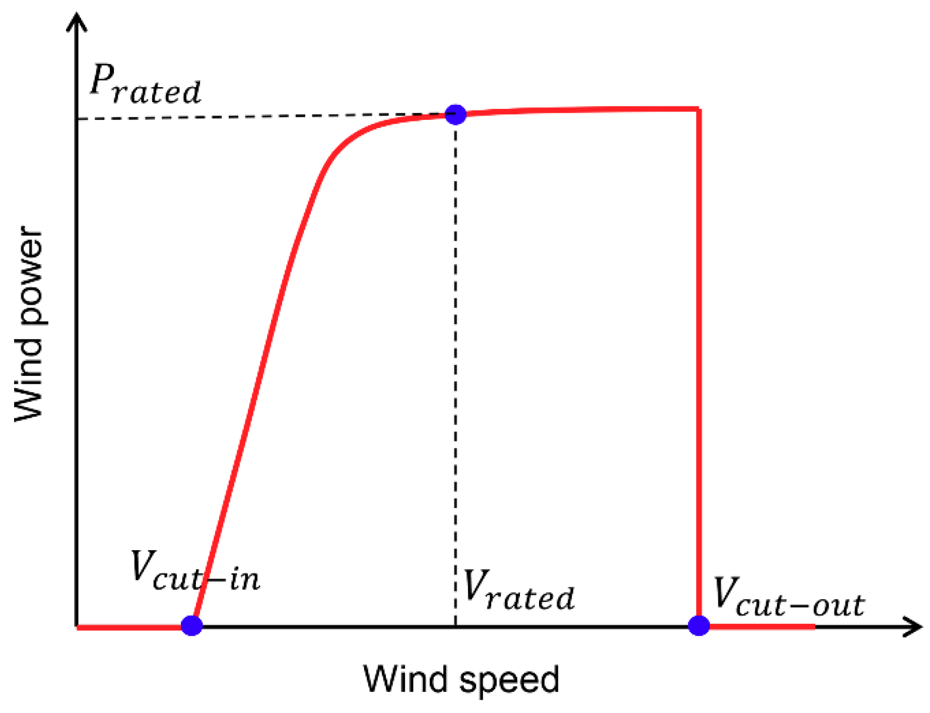
2. Popular Power Curve Models

In this section, some popular power curve models are introduced briefly. Usually, they can be divided into two categories: parametric models and nonparametric models.

2.1. Parametric Models

Parametric models, which are constructed by several mathematic expressions with several parameters, are often used to describe the WTPC [23]. Some representative parametric models such as 3-PLF, 4-PLF, 5-PLF, 6-PLF, and MHTan are introduced here. Supposing $V,P$ represent wind speed and wind power, respectively, the calculations of different parametric models are presented in

Table 1. Parametric wind turbine power curve models.

Model	Expression	Parameters
3-PLF	$P=\frac{k{y}_0{e}^{rV}}{k+y_0\left(e^{rV}-1\right)}$	$k$: the capacity of the system; $r$: the rate of increase; $y_0$: no special mean.
4-PLF	$P=\alpha +\frac{\beta -\alpha }{1+{\left(\frac{V}{\gamma }\right)}^{\delta }}$	$\alpha$: the maximum asymptote; $\beta$: the minimum asymptote; $\gamma$: the inflection point, $\delta$: means the hill slope.
5-PLF	$P=\alpha +\frac{\left(\beta -\alpha \right)}{{\left(1+{\left(\frac{V}{\gamma }\right)}^{\delta }\right)}^{ϵ}}$	$ϵ$: the asymmetric factor; $\alpha ,\beta ,\gamma ,\delta$ are the same with the parameters in 4-PLF.
6-PLF	$P=\delta +\frac{\alpha -\delta }{{\left(ϵ+\exp \left(-\beta \left(V-V_0\right)\right)\right)}^{1/\gamma }}$	$\delta$: the lower asymptote; $\alpha$: the upper asymptote; $\beta$: the growth rate; $\gamma$: the closet asymptote to the maximum growth part of the curve; $V_0$: the value $P\left(0\right)$; $ϵ$: the value around 1.
MHTan	$P=\frac{{\alpha }_1{e}^{{\alpha }_{2}V}-{\alpha }_3{e}^{-{\alpha }_{4}V}}{{\alpha }_5{e}^{{\alpha }_{6}V}-{\alpha }_7{e}^{-{\alpha }_{8}V}}+{\alpha }_9$	${\alpha }_1,{\alpha }_2,\cdots ,{\alpha }_9$: nine model parameters.

.

As for 5-PLF, it can degenerate in 4-PLF when the asymmetric factor $ϵ$ is equal to 1. MHTan can degenerate into a hyperbolic tangent by assuming ${\alpha }_1=\cdots ={\alpha }_8=1$ and ${\alpha }_9=0$, while it becomes a hyperbolic sine when ${\alpha }_1=\cdots ={\alpha }_5={\alpha }_7=1$ and ${\alpha }_6={\alpha }_8={\alpha }_9$ [10].

2.2. Nonparametric Models

For a wind turbine, there is a nonlinear relationship between power output and the other variables, such as wind speed and wind direction. It is usually described by a wind turbine power curve and expressed by the following function, namely.

$$P=f\left(V,\mathit{\theta }\right)+\zeta$$

(1)

where $\mathit{\theta }$ denotes the set of variables that affect the power output of a wind turbine, such as wind direction and pressure, $\zeta$ is the error term, $f(\cdot )$ is the nonlinear function.

Due to the superior nonlinear fitting ability of many artificial intelligence methods, they have been widely utilized in wind turbine power curve modeling, namely estimating the unknown nonlinear function $f(\cdot )$. Some popular ones are SVR [20], GP [21,22], and ANNs [19,26].

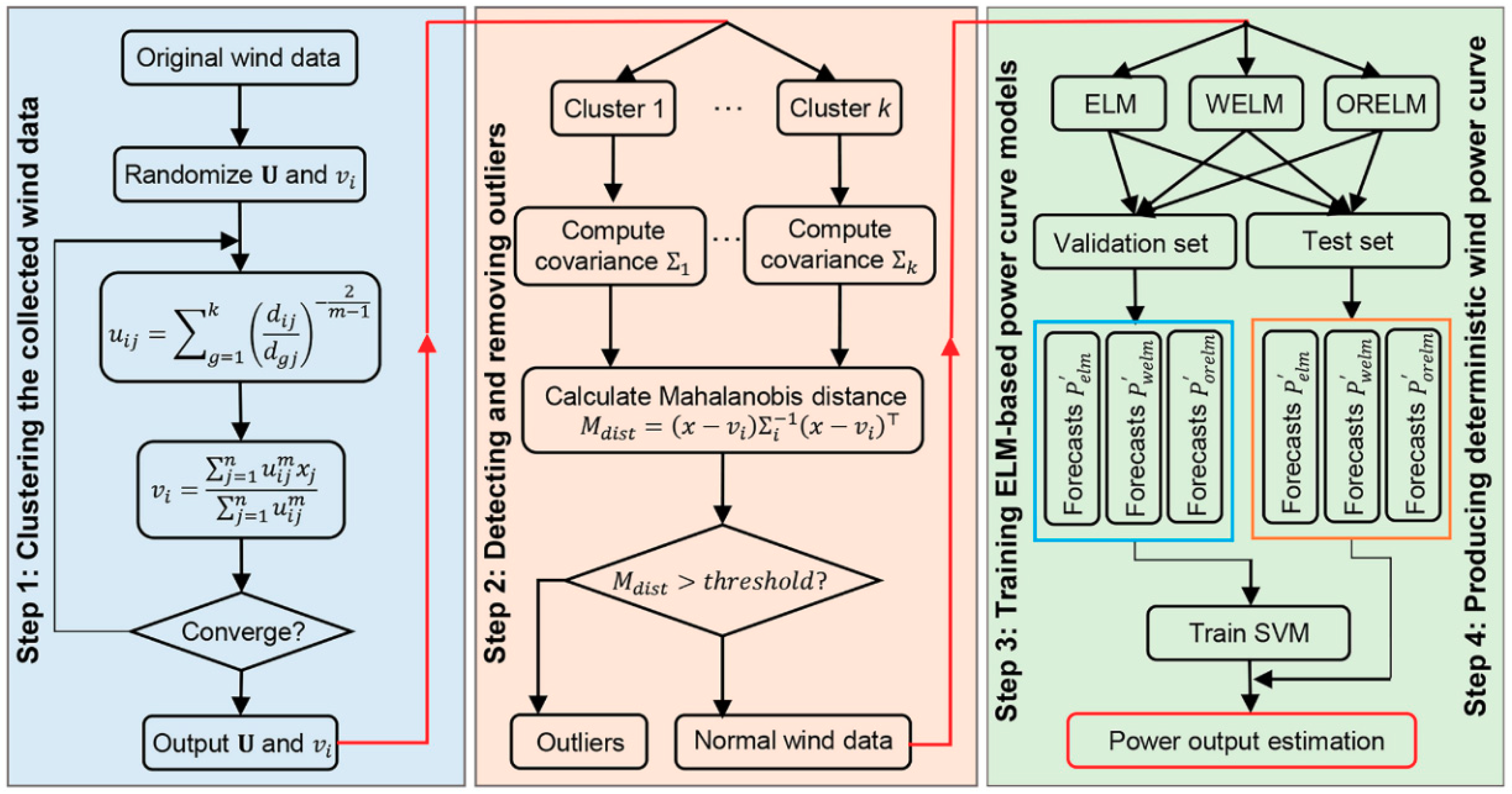
3. Proposed Wind Power Curve Model

In this section, related methods for the proposed model are introduced at first. Then, the proposed strategies for deterministic and probabilistic power curve modeling are presented in detail.

3.1. Fuzzy C-Means Clustering

FCM was first proposed by Bezdek in 1981 [39]. In FCM, each sample is not strictly divided into a certain class. It has a degree of membership for each class. Generally, the objective function for FCM can be expressed as [40]

$$J_m\left(U,v_1,\cdots ,v_k\right)={\displaystyle \sum }_{i=1}^k{J}_i={\displaystyle \sum }_{j=1}^n{\displaystyle \sum }_{i=1}^k{u}_{ij}^m{d}_{ij}^2$$

(2)

where the membership matrix $U={\left\{u_{ij}\right\}}_{k\times n}$, $1\le i\le k$, $1\le j\le n$, $\left\{v_1,\dots ,v_k\right\}$ are $k$ cluster centers, $n$ is the number of samples, $m$ is the weighting exponent, and its value is usually selected as 2, $u_{ij}$ denotes the degree that the $j$th sample belongs to the $i$th cluster, $0<u_{ij}<1$, ${{\displaystyle \sum }}_{i=1}^k{u}_{ij}=1$, $d_{ij}=\left|\left|x_j-v_i\right|\right|$ is the Euclidean distance between the sample $x_j$ and the cluster center $v_i$.

Considering the constraint on $u_{ij}$, the objective function can be rewritten as the following function by introducing a Lagrange multiplier $\lambda$,

$$F={\displaystyle \sum }_{j=1}^n{\displaystyle \sum }_{i=1}^k{u}_{ij}^m{d}_{ij}^2+\lambda \left(1-{\displaystyle \sum }_{i=1}^k{u}_{ij}\right)$$

(3)

Let the partial derivatives of function $F$ with respect to $u_{ij}$ and $v_i$, respectively, equal to 0, the updated formulas for $u_{ij}$ and $v_i$ can be expressed as [40]

$$u_{ij}={\left[{\displaystyle \sum }_{g=1}^k{\left(\frac{d_{ij}}{d_{gj}}\right)}^{\frac{2}{m-1}}\right]}^{-1}$$

(4)

$$v_i=\frac{{{\displaystyle \sum }}_{j=1}^n{u}_{ij}^m{x}_j}{{{\displaystyle \sum }}_{j=1}^n{u}_{ij}^m}$$

(5)

FCM employs the above two functions to update the membership matrix $U$ and all cluster centers so as to make the objective function reach its minimum.

3.2. Extreme Learning Machine and Its Variants

In this subsection, the original ELM and its variants are introduced briefly.

3.2.1. Extreme Learning Machine

ELM is a new single hidden layer feed-forward neural network that was first proposed by Huang et al. [35] in 2004. Given the $i$th sample pair $\left\{X_i,T_i\right\}\left(i=1,\cdots ,N\right)$, where $X_i={\left[x_{i1},x_{i2},\cdots ,x_{iD}\right]}^T\in R^D$ is the output of ELM with $M$ hidden nodes is given by

$$f\left(X_i\right)={\displaystyle \sum }_{m=1}^M{\beta }_m H\left({\varpi }_m,X_i,{\alpha }_m\right)$$

(6)

where $H(\cdot )$ is the activation function, ${\beta }_m$ is the $m$th output weight, ${\varpi }_m\in R^D$ is the input weight vector, and ${\alpha }_m$ is the corresponding bias. Equation (6) can be re-written as a matrix form,

$$\widehat{T}=H\beta$$

(7)

where $\beta ={\left[{\beta }_1,{\beta }_2,\cdots ,{\beta }_M\right]}^T\in R^M$ is the output weight vector, the output vector $\widehat{T}={\left[f\left(X_i\right),\cdots ,f\left(X_N\right)\right]}^T\in R^N, H\in R^{N\times M}$ is the hidden layer output matrix, which is represented as

$$=\left[\begin{array}{ccc}H\left(\varpi ,X_1,{\alpha }_1\right)& \cdots & H\left(\varpi ,X_1,{\alpha }_M\right)\\ ⋮& \ddots & ⋮\\ H\left(\varpi ,X_N,{\alpha }_1\right)& \cdots & H\left(\varpi ,X_N,{\alpha }_M\right)\end{array}\right]$$

(8)

The optimization of ELM is to solve the following minimization problem,

$$\underset{\beta }{\min }\Vert H\beta -T{\Vert }_2^2=\underset{\beta }{\min }\Vert H\beta -T{\Vert }_2^2$$

(9)

where $T={\left[T_1,\cdots ,T_N\right]}^T\in R^N$ is the observed target matrix, $\Vert \cdot {\Vert }_2^2$ denotes the squared $l_2$-norm of a vector. Then, the output weight vector $\beta$ can be estimated by

$$\beta =H^{†}T$$

(10)

where $H^{†}$ denotes the Moore–Penrose generalized inverse of $H$.

3.2.2. Weighted Regularized Extreme Learning Machine (WELM)

The objective function for a regularized ELM can be expressed as [41]

$$\begin{array}{c}\underset{\beta }{\mathrm{argmin}} C{\left|\left|\epsilon \right|\right|}_2^2+{\left|\left|\beta \right|\right|}_2^2\\ s.t. T=H\beta +\epsilon \end{array}$$

(11)

where $C$ is the regularization term. By introducing a vector of Lagrangian multiplier $\alpha \in R^N$, the corresponding Lagrangian function is defined as

$$L\left(\beta ,\epsilon ,\alpha \right)={\Vert \epsilon \Vert }_2^2+C{\Vert \beta \Vert }_2^2+{\alpha }^T\left(T-H\beta -\epsilon \right)$$

(12)

The corresponding solution for the above problem is [37,41]

$$\beta ={\left(H^{T}H+\frac{I}{C}\right)}^{-1}{H}^{T}T$$

(13)

where $I$ is an identity matrix.

Deng et al. [36] developed a WELM to reduce the adverse effects of outliers. They weighted the $i$th error term ${\epsilon }_i$ by the weighting factor ${\eta }_i$. Thus, the error term ${\Vert \epsilon \Vert }_2^2$ in Equation (11) becomes ${\Vert \eta \epsilon \Vert }_2^2$. The objective function for WELM is expressed as [36,37]

$$\begin{array}{c}\underset{\beta }{\mathrm{argmin}} C{\Vert \eta \epsilon \Vert }_2^2+{\Vert \beta \Vert }_2^2\\ s.t. T=H\beta +\epsilon \end{array}$$

(14)

where $\eta =diag\left\{{\eta }_1,\cdots ,{\eta }_N\right\}$ is a diagonal matrix. Similar to the optimization of the regularized ELM, Lagrangian multiplier is also introduced. The solution for WELM is given by [36,37]

$$\beta ={\left(H^T{\eta }^{2}H+\frac{I}{C}\right)}^{-1}{H}^T{\eta }^{2}T$$

(15)

There are several weighting functions that can be used to construct weighting matrix $\eta$, as suggested in [36,37,41], the expression of Hampel weighting function is given by

$${\eta }_i=\{\begin{array}{c}1 \left|{\epsilon }_i/\widehat{s}\right| \le c_1\\ \frac{c_2-\left|{\epsilon }_i/\widehat{s}\right|}{c_2-c_1} c_1<\left|{\epsilon }_i/\widehat{s}\right|<c_2\\ {10}^{-4} otherwise\end{array}$$

(16)

where $\widehat{s}$ is the robust estimate of the standard deviation of the error variables generated by the regularized ELM,

$$\widehat{s}=\frac{IQR}{2\times 0.6745}$$

(17)

The term IQR denotes the inter-quartile range, which is the difference between the 75th percentile and the 25th percentile. And, the constants $c_1$, $c_2$ are typically set as $c_1=2.5$ and $c_2=3$ [37].

On the whole, there are three steps to construct a WELM model. Firstly, the regularized ELM model is used to generate the error series $\left\{{\epsilon }_1,\cdots ,{\epsilon }_N\right\}$. Secondly, according to the computed error series, the weighting matrix will be calculated by Equation (16). Finally, the output weight vector $\beta$ is obtained via Equation (15).

3.2.3. Outlier-Robust Extreme Learning Machine (ORELM)

Owing to the presence of outliers, the training error will show the sparse characteristic [37]. The sparsity can be realized by $l_0$-norm rather than $l_2$-norm. So, to deal with outliers, the objective function can be modified by replacing ${\Vert E\Vert }_2^2$ with ${\Vert E\Vert }_0$. However, the modified objective function becomes a non-convex problem, which is difficult to be optimized. With this in mind, Zhang and Luo [37] replaced ${\Vert \epsilon \Vert }_0$ by the $l_1$-norm-based loss function, ${\Vert E\Vert }_1$. Thus, the objective function is given by

$$\begin{array}{c}\underset{\beta }{\mathrm{argmin}} {\Vert \epsilon \Vert }_1+\frac{1}{C}{\Vert \beta \Vert }_2^2\\ s.t. T=H\beta +\epsilon \end{array}$$

(18)

For Equation (18), it not only guarantees the sparsity, but also leads to the overall minimization convex [37]. Then, the Augmented Lagrange Multiplie (ALM) method is used to optimize Equation (18), and the corresponding Lagrangian function is expressed as

$$L\left(\epsilon ,\beta ,\alpha \right)={\Vert \epsilon \Vert }_1+\frac{1}{C}{\Vert \beta \Vert }_2^2+{\alpha }^T\left(T-H\beta -\epsilon \right)+\frac{\mu }{2}{\Vert T-H\beta -\epsilon \Vert }_2^2$$

(19)

where $\mu$ is a penalty parameter and set as $\mu =2N/{\Vert T\Vert }_1$ in [37]. The optimal solutions for $\epsilon$, $\beta$, $\alpha$ can be obtained by iteratively minimizing Equation (19). The corresponding iterative functions are

$$\begin{gathered} {\beta }_{k+1}={\left(H^{T}H+\frac{2}{C\mu I}\right)}^{-1}{H}^T\left(T-{\epsilon }_k+\frac{{\alpha }_k}{\mu }\right) \\ {\epsilon }_{k+1}=max\left\{\left|T-H{\beta }_{k+1}+\frac{{\alpha }_k}{\mu }\right|-\frac{1}{\mu },0\right\}\circ sign\left(T-H{\beta }_{k+1}+\frac{{\alpha }_k}{\mu }\right) \\ {\alpha }_{k+1}={\alpha }_k+\mu \left(T-H{\beta }_{k+1}-{\epsilon }_{k+1}\right) \end{gathered}$$

(20)

where $\circ$ means the element-wise multiplication, and $sign (\cdot )$ is a sign function. The optimal output weights $\beta$ can be obtained when the number of iterations reaches a predefined maximum iteration [37].

3.3. Support Vector Regression

SVR was first proposed by Vapnik based on the structural risk minimization [38]. The main idea is to find a nonlinear mapping function $\varphi$, which can map low-dimensional data into high-dimensional feature space.

Given the training data $\left\{\left(x_1,y_1\right),\left(x_2,y_2\right),\cdots ,\left(x_n,y_n\right)\right\}$, the aim is to get an estimated $f\left(x\right)$ for the real output $y$, the expression of $f\left(x\right)$ is $f\left(x\right)=w^T\varphi \left(x\right)+b$, in which $w$, $b$ are two model parameters. The objective function for SVR is

$$\underset{w,b}{\min }\frac{1}{2}{\Vert w\Vert }^2+C{\displaystyle \sum }_{i=1}^{n}l\left(f\left(x_i\right)-y_i\right)$$

(21)

where $l(\cdot )$ is the loss function, $C$ is the trade-off parameter. For the original SVR, the $\epsilon$-insensitive loss function is employed. When introducing the slack variables ${\xi }_i$, ${\xi }_i^{*}$, the primal problem for SVR is

$$\begin{array}{c}\underset{w,b,{\xi }_i,{\xi }_i^{*}}{\min }\frac{1}{2}{\Vert w\Vert }^2+C{\displaystyle \sum _{i=1}^n}\left({\xi }_i+{\xi }_i^{*}\right)\\ s.t. \{\begin{array}{c}{y}_i-\left(w^T\varphi \left(x_i\right)+b\right)<\epsilon +{\xi }_i\\ \left(w^T\varphi \left(x_i\right)+b\right)-y_i<\epsilon +{\xi }_i^{*}\\ {\xi }_i,{\xi }_i^{*}\ge 0\end{array}\end{array}$$

(22)

The dual problem for SVR can be obtained by applying the Karush-Kuhn-Tucker (KKT) conditions. Then, the decision function $f\left(x\right)$ for a new sample $x$ is

$$f\left(x\right)={\displaystyle \sum }_i^n\left({\alpha }_i-{\alpha }_i^{*}\right)K\left(x,x_i\right)+b$$

(23)

where $K\left(x,x_i\right)=\langle \varphi \left(x\right),\varphi \left(x_i\right)\rangle$ is the kernel function, ${\alpha }_i,{\alpha }_i^{*} \left(i=1,\cdots ,n\right)$ denote the Lagrangian multipliers. Usually, Gaussian kernel is used in many applications due to its superior performance.

3.4. Proposed Strategy for Wind Power Curve Modeling

In our collected wind data, there are many outliers, which may be caused by over dating, pitch malfunction, pitch controller malfunction, wind speed under reading, dirt, bugs or icing on blades, and down rating, and so on. [42]. So, it is essential to detect and remove those outliers in our collected wind data. In this paper, several steps, which are described in Figure 2, are taken to generate accurate wind power curves.

Step 1: Clustering the collected wind data. Different environmental conditions or different working conditions lead to different patterns and characteristics of the collected wind data. Here, FCM is employed to divide the data into different clusters. The samples in the same cluster may have some common characteristics.

Step 2: Detecting and removing outliers. In a certain cluster, Mahalanobis distance is employed to measure the distance between the sample and cluster center. Generally, outliers will be far from normal samples, and also farther from the cluster center than normal samples. So, the sample will be considered as an outlier when the distance between the sample and cluster center is larger than a given threshold. Then, the detected outliers will be removed from the data. The Mahalanobis distance can be computed by

$$M_{dist}=\left(x-\mu \right){\Sigma }^{-1}{\left(x-\mu \right)}^{\top }$$

(24)

where $x$ is the sample in the observed cluster, $\mu ,\mathsf{\Sigma }$ are the corresponding cluster center and covariance of all samples in the same cluster.

Step 3: Training ELM-based power curve models. After removing the outliers from the collected data, the processed data is employed to train different wind power curve models. However, one cannot ensure that all outliers are detected and removed from the collected wind data. So, some unobvious outliers may hide in the processed data. It is wise to use robust wind power curve models to eliminate the adverse effect of hidden outliers on the power curve modeling. Moreover, considering the efficiency of ELM, the original ELM and its two robust variants are selected as basic power curve models to describe the nonlinear relationship between wind speed and power output. The number of hidden nodes in ELM-based models greatly affects their performance. So, in their training phases, validation sets are employed to help select the optimal model parameters, which can be obtained when the forecasting error on a validation set reaches its minimum.

Step 4: Producing deterministic wind power curve. Occasionally, a single model is unable to describe the complex relationship comprehensively. So, in this paper, alongside the wind speed, the wind power forecasts on the validation set obtained in Step 3 are also used as inputs to train a regression model, SVR. Namely, SVR is utilized to approximate the function $f(\cdot )$ in the following equation,

$$P_{real}=f\left(S,P_{elm}^{\prime },P_{welm}^{\prime },P_{orelm}^{\prime }\right)+\epsilon$$

(25)

where $P_{real}$ is the real wind power, $P_{elm}^{\prime }$, $P_{welm}^{\prime }$, $P_{orelm}^{\prime }$ denote the forecasted wind power obtained by ELM, WELM, and ORELM, respectively, at wind speed $V$, $\epsilon$ is the error term. Then, at any unknown wind speed, the corresponding wind power forecasts can be obtained using the trained SVR. Thus, a deterministic wind power curve can be derived.

4. Wind Turbine Power Curve Modeling in Different Wind Farms

In this section, to evaluate the performances of different power curve models under various geographical environments, a comparative study is conducted in different wind farms.

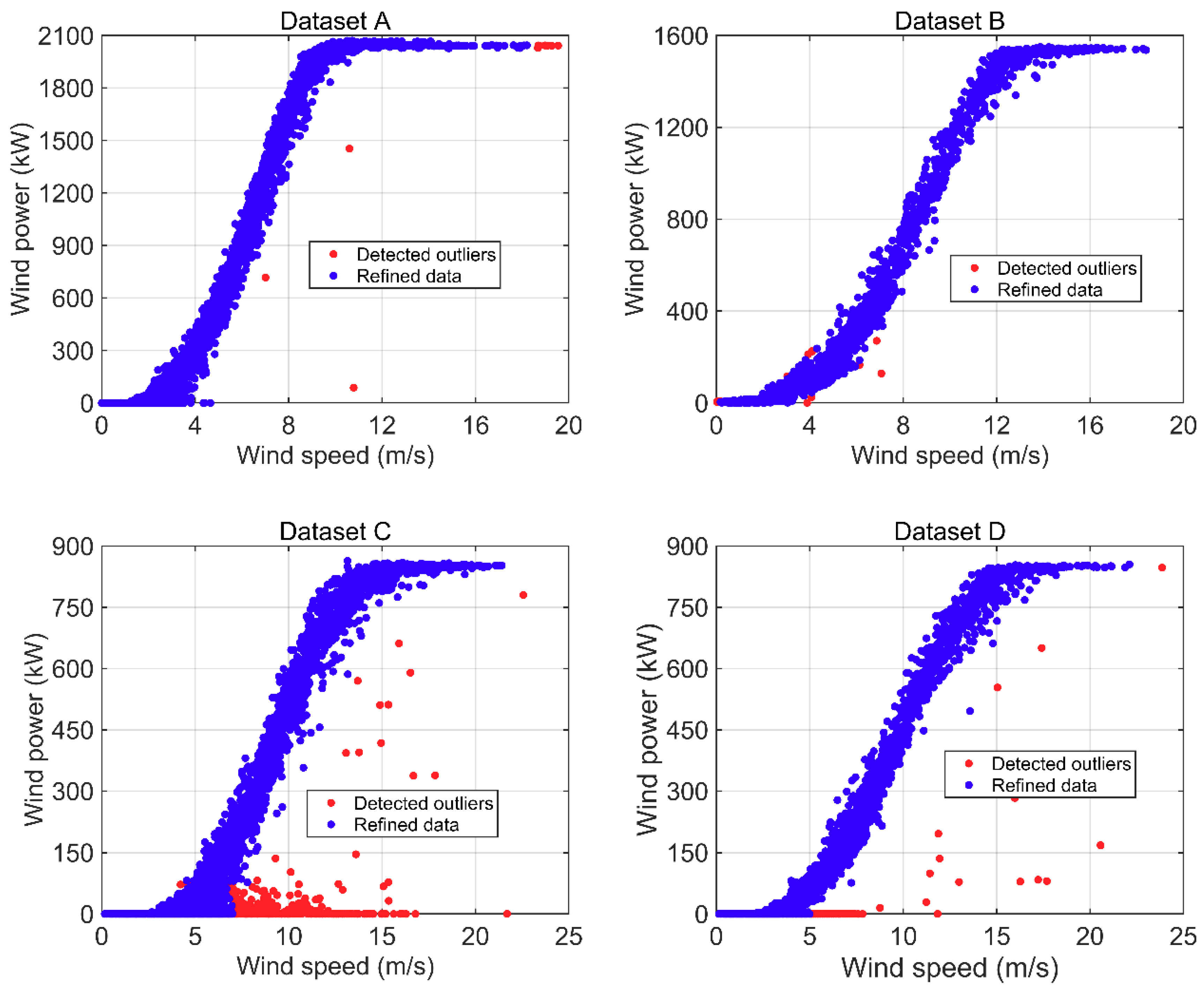
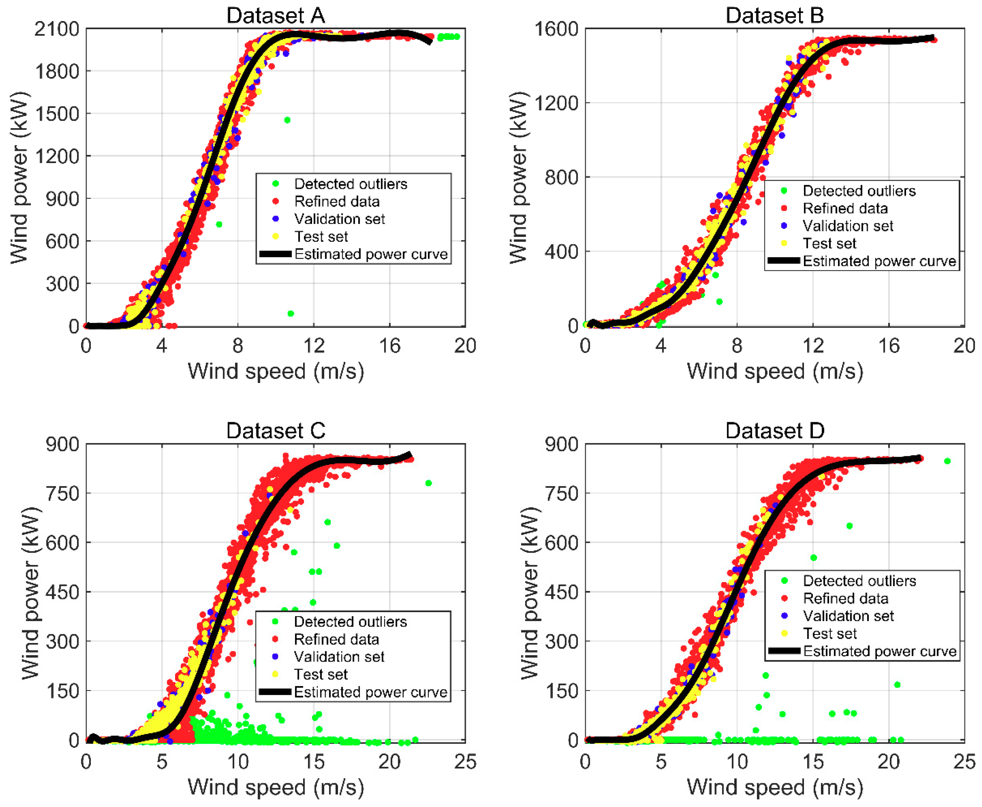
4.1. Data Description

Four wind datasets were taken to assess the performance of different power curve models. Dataset A and Dataset B were collected from China Xichang and Hunan wind farms, respectively. For Dataset C and Dataset D, they were collected from different wind turbines of the same wind farm. The whole dataset for each wind farm was divided into three separate parts: training set, validation set, and test set. The training set was used to train different power curve models, the validation set was employed to select the optimal model parameters, and the performances of different models were evaluated on the test set. The information of four datasets is presented in

Table 2. The numbers of different types of samples in four datasets.

Dataset	All Samples (#)	Training Samples (#)	Validation Samples (#)	Test Samples (#)
A	5500	4500	400	600
B	6500	5500	400	600
C	7500	6000	500	1000
D	6000	5000	400	600

. In all datasets, only two variables, wind speed and wind power, were measured and reserved. So, the only input for all power curve models is wind speed.

4.2. Experiment Setting

In order to make a comparative study comprehensively, five parametric models (e.g., 3-PLF, 4-PLF, 5-PLF, 6-PLF and MHTan) and five nonparametric models, back-propagation neural network (BPNN), ANFIS, ELM, WELM, ORELM, were utilized. For all models, the only input was wind speed, and the output was wind power. Moreover, all models were trained with the same processed data generated by the FCM-based model for a fair comparison.

In the paper, similar to [10], the backtracking search algorithm (BSA) was employed to optimize the model parameters in all parametric models with the least squares loss function. Grid search was employed to tune the parameters in SVR. For BPNN, the number of neurons in hidden layers are determined by the Hecht-Nelson method [9]. For ELM-based regression models, the optimal number of hidden layers can be obtained when the modeling error of the observed model on the validation set reaches the minimum. The candidate number of hidden layers can be selected from the set $\left\{20,40,60,\cdots ,200\right\}$.

In order to test the performances of different models, four error indicators, mean absolute error (MAE), root mean square error (RMSE), normalized mean absolute percentage error (NMAPE) and the coefficient of determination ($R^2$), were employed. For all models, the values of different error indicators were computed based on the same test set. Assuming that $y_l$ denotes the lth measured value in the test set, and $\widehat{y_l}$ is the corresponding forecast ($l=1,\cdots ,L$), $\overline{y_l}$ is the mean of all measured values, $L$ is the number of samples in the test set, the calculations for the four error indicators are presented in

Table 3. Performance evaluation metrics and the corresponding definitions.

Indicator	Calculation	Description
MAE	$MAE={\displaystyle \sum _{l=1}^L}\frac{\left|y_l-\widehat{y_l}\right|}{L}$	The smaller the better
RMSE	$RMSE=\sqrt{{\displaystyle \sum _{l=1}^L}\frac{{\left(y_l-\widehat{y_l}\right)}^2}{L}}$	The smaller the better
NMAPE	$NMAPE=\frac{1}{L}{\displaystyle \sum _{l=1}^L}\frac{\left|y_l-\widehat{y_l}\right|}{\max \left\{y_1,\cdots ,y_L\right\}}\times 100\%$	The smaller the better
$R^2$	$R^2=1-\frac{{{\displaystyle \sum }}_{l=1}^L{\left(y_l-\widehat{\left(y_l\right)}\right)}^2}{{{\displaystyle \sum }}_{l=1}^L{\left(y_l-\overline{\left(y_l\right)}\right)}^2}$	The bigger the better

. For MAE, NMAPE and RMSE, a smaller value indicates a better estimator. However, the closer the value of $R^2$ is to 1, the better the model.

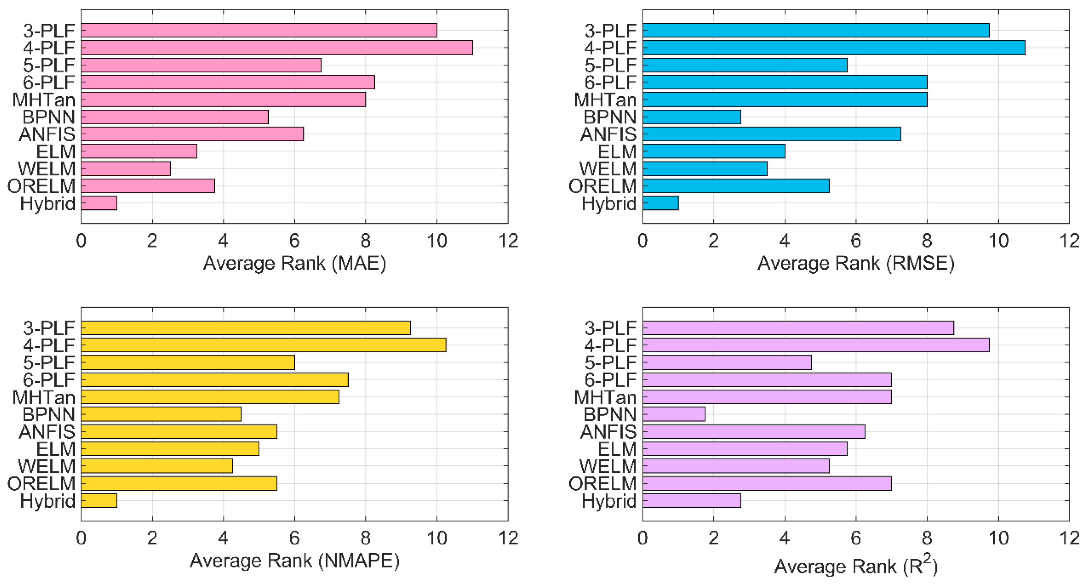
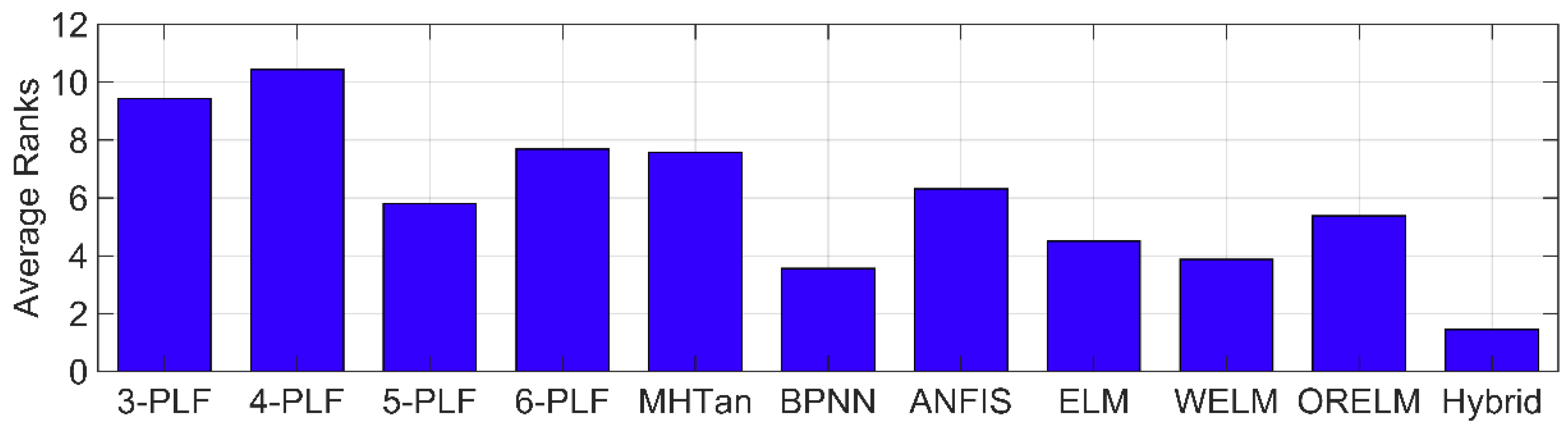
4.3. Results of Wind Turbine Power Curve Modeling

According to the steps described in Section 3.3, the original wind data are clustered by FCM at first. Then, in each cluster, if the Mahalanobis distance (Equation (24)) is larger than 10, the sample will be considered as outliers. The refined data and outliers are presented in Figure 3. From Figure 3, most outliers can be detected from the original wind data by FCM-based outlier detection model.

After some outliers are detected and removed from four datasets, the processed wind data will be used to train different power curve models. For ELM-based power curve models, the number of neurons in hidden layers has a great effect on their performance. So, the validation set in each dataset helps to select the optimal number of neurons in the given candidates. In four datasets, as the number of neurons in hidden layers changed, the performances of ELM-based power curve models on the validation set were calculated, and these are presented in

Table 4. Power curve modeling results of ELM-based models on validation set of Dataset A.

Number of Neurons	ELM		WELM		ORELM
	MAE	NMAPE	MAE	NMAPE	MAE	NMAPE
20	31.1966	1.5165	30.6275	1.4889	30.2793	1.4720
40	31.3355	1.5233	30.6819	1.4915	30.1564	1.4660
60	31.2018	1.5168	30.6325	1.4891	30.0923	1.4629
80	31.2489	1.5191	30.5587	1.4855	30.0131	1.4590
100	31.1304	1.5133	30.5600	1.4856	30.1424	1.4653
120	31.1159	1.5126	30.5568	1.4854	30.0607	1.4613
140	31.1660	1.5151	30.5901	1.4871	30.1577	1.4660
160	31.2230	1.5178	30.6028	1.4877	30.2313	1.4696
180	31.2163	1.5175	30.7079	1.4928	30.2346	1.4698
200	31.2042	1.5169	30.6600	1.4905	30.2831	1.4721

,

Table 5. Power curve modeling results of ELM-based models on validation set of Dataset B.

Number of Neurons	ELM		WELM		ORELM
	MAE	NMAPE	MAE	NMAPE	MAE	NMAPE
20	19.5752	1.2916	19.6813	1.2986	19.3721	1.2782
40	19.4678	1.2845	19.3994	1.2800	19.1576	1.2640
60	19.5612	1.2906	19.6308	1.2952	19.4058	1.2804
80	19.5769	1.2917	19.6576	1.2970	19.3674	1.2778
100	19.5334	1.2888	19.5756	1.2916	19.4176	1.2812
120	19.5381	1.2891	19.6577	1.2970	19.9057	1.3134
140	19.5528	1.2901	19.6811	1.2985	19.9866	1.3187
160	19.5555	1.2903	19.7093	1.3004	20.1874	1.3319
180	19.5723	1.2914	19.6612	1.2972	19.7598	1.3037
200	19.5538	1.2901	19.6977	1.2996	20.1378	1.3287

,

Table 6. Power curve modeling results of ELM-based models on validation set of Dataset C.

Number of Neurons	ELM		WELM		ORELM
	MAE	NMAPE	MAE	NMAPE	MAE	NMAPE
20	15.3341	2.0665	15.3846	2.0733	16.0515	2.1631
40	15.4442	2.0813	15.6734	2.1122	16.0831	2.1674
60	15.4285	2.0792	15.4668	2.0843	16.1864	2.1813
80	15.4258	2.0788	15.4991	2.0887	16.3482	2.2031
100	15.4324	2.0797	15.4687	2.0846	16.2203	2.1859
120	15.2910	2.0606	15.3831	2.0731	15.7288	2.1196
140	15.4222	2.0783	15.7103	2.1172	16.3020	2.1969
160	15.4347	2.0800	15.4756	2.0855	16.2555	2.1906
180	15.4334	2.0798	15.4823	2.0864	16.2622	2.1915
200	15.2928	2.0609	15.5146	2.0908	15.7213	2.1186

and

Table 7. Power curve modeling results of ELM-based models on validation set of Dataset D.

Number of Neurons	ELM		WELM		ORELM
	MAE	NMAPE	MAE	NMAPE	MAE	NMAPE
20	9.7527	1.3681	9.7187	1.3634	9.6653	1.3559
40	9.7582	1.3689	9.7191	1.3634	9.6651	1.3559
60	9.7528	1.3682	9.7150	1.3629	9.6692	1.3564
80	9.7583	1.3689	9.7179	1.3633	9.6574	1.3548
100	9.7594	1.3691	9.7182	1.3633	9.6615	1.3554
120	9.7593	1.3691	9.7186	1.3634	9.6631	1.3556
140	9.7529	1.3682	9.7156	1.3629	9.6688	1.3564
160	9.7603	1.3692	9.7197	1.3635	9.6594	1.3551
180	9.7592	1.3691	9.7186	1.3634	9.6584	1.3549
200	9.7587	1.3690	9.7188	1.3634	9.6601	1.3552

.

From Table 4, in Dataset A, the optimal numbers of hidden nodes for ELM, WELM, and ORELM are 120, 120 and 80, respectively. According to the results in Table 5, 40, 40, and 40 were selected as the optimal numbers of hidden nodes in ELM, WELM, and ORELM, respectively, for Dataset B. From Table 6, the optimal ones are 120, 120, and 200 for Dataset C, while from Table 7, they are 20, 60, and 80 for Dataset D. After the optimal numbers of hidden nodes in ELM-based models were decided, the trained models were used to forecast the power output of a wind turbine at an unknown wind speed. The results of ELM, WELM, and ORELM in different datasets are presented in

Table 8. Results of all power curve models on test sets of Dataset A and Dataset B.

Dataset	Model	Error Indicator
		MAE	RMSE	NMAPE	${\mathit{R}}^{\mathbf{2}}$
A	3-PLF	48.4476	63.2152	2.3528	0.9949
	4-PLF	48.7739	63.4799	2.3686	0.9948
	5-PLF	36.5998	53.3506	1.7774	0.9963
	6-PLF	45.2280	60.8805	2.1964	0.9952
	MHTan	42.7914	58.3378	2.0781	0.9956
	BPNN	32.1661	51.2157	1.5621	0.9966
	ANFIS	37.3980	53.3276	1.8162	0.9963
	ELM	32.0219	51.4542	1.5551	0.9966
	WELM	31.6347	52.3488	1.5363	0.9965
	ORELM	31.6811	53.6236	1.5385	0.9963
	Hybrid	30.5422	49.7355	1.4832	0.9968
B	3-PLF	21.7192	34.9560	1.4212	0.9891
	4-PLF	21.7790	34.9837	1.4251	0.9891
	5-PLF	19.9222	33.2145	1.3036	0.9902
	6-PLF	20.6772	34.6191	1.3530	0.9894
	MHTan	20.5743	34.2099	1.3463	0.9896
	BPNN	19.3444	32.8101	1.2658	0.9904
	ANFIS	19.3400	33.7645	1.2655	0.9899
	ELM	19.2145	32.9260	1.2573	0.9904
	WELM	19.2872	33.2975	1.2620	0.9902
	ORELM	19.7225	34.2069	1.2905	0.9896
	Hybrid	18.8438	32.0968	1.2330	0.9909

and

Table 9. Results of all power curve models on test sets of Dataset C and Dataset D.

Dataset	Model	Error Indicator
		MAE	RMSE	NMAPE	${\mathit{R}}^{\mathbf{2}}$
C	3-PLF	21.7192	34.9560	1.4212	0.9891
	4-PLF	21.7790	34.9837	1.4251	0.9891
	5-PLF	19.9222	33.2145	1.3036	0.9902
	6-PLF	20.6772	34.6191	1.3530	0.9894
	MHTan	20.5743	34.2099	1.3463	0.9896
	BPNN	19.3444	32.8101	1.2658	0.9904
	ANFIS	19.3400	33.7645	1.2655	0.9899
	ELM	16.0682	26.9427	2.1093	0.9425
	WELM	15.8361	26.6344	2.0788	0.9438
	ORELM	15.9102	25.9158	2.0885	0.9468
	Hybrid	9.0638	16.4979	1.1898	0.9784
D	3-PLF	15.0039	19.0627	1.8723	0.9811
	4-PLF	15.0733	19.1098	1.8810	0.9810
	5-PLF	10.1637	16.9569	1.2683	0.9850
	6-PLF	10.1192	16.5730	1.2628	0.9857
	MHTan	11.1313	17.3347	1.3891	0.9844
	BPNN	10.0238	16.3810	1.2509	0.9860
	ANFIS	11.4776	20.5935	1.4323	0.9779
	ELM	9.8328	16.6137	1.2270	0.9856
	WELM	9.8043	16.4880	1.2235	0.9858
	ORELM	9.7503	16.5073	1.2167	0.9858
	Hybrid	9.4122	16.1494	1.1745	0.9864

.

According to the Step 4 of the proposed hybrid model described in Section 3.3, the wind power forecasts of the optimal ELM, WELM, and ORELM on the validation set are used as inputs, together with the corresponding wind speed, to train SVR. Then, the forecasted power output can be obtained by the trained SVR. The results are presented in Table 8 and Table 9. Moreover, the results of the other ten compared models (five parametric models and five nonparametric models) are also shown in Table 8 and Table 9.

According to Table 8, the proposed hybrid model provides better power forecasts than the other compared models in Dataset A. Moreover, the majority of nonparametric models outperform parametric models. However, 5-PLF performs better than ANFIS. In five parametric models, 5-PLF is the best one. With the exception of the hybrid model, among the five nonparametric models, no model outperforms the others in terms of four error indicators. Specifically, WELM performs the best in terms of MAE and NMAPE, while the best one is BPNN in terms of RMSE and $R^2$.

From the results on Dataset B and Dataset D presented in Table 8 and Table 9, respectively, the best model is also the proposed hybrid model in terms of all error indicators. Similar to the results in Dataset A, most nonparametric models perform better than parametric models. Among all parametric models, 5-PLF usually generates better power forecasts.

According to the results in Dataset C presented in Table 9, the proposed hybrid model is superior to the other models in terms of MAE, RMSE, and NMAPE, while BPNN is the best model in terms of $R^2$. Moreover, in terms of MAE and RMSE, ELM, WELM, and ORELM perform better than the other compared models. However, in terms of NMAPE and $R^2$, ELM, WELM, and ORELM perform worse than the other compared models.

According to the results in Table 8 and Table 9, the average ranks of all wind turbine power output estimation models were computed, and these are presented in Figure 4. From Figure 4, according to different error indicators, the average ranks of wind turbine power output models are also different. In terms of the MAE, RMSE, and NMAPE, the proposed hybrid model ranks the highest among all models. However, in terms of $R^2$, BPNN ranks first and the proposed hybrid model ranks second. Moreover, in terms of MAE and NMAPE, all nonparametric models rank higher than all parametric models. In terms of RMSE, except the ANFIS, all nonparametric models perform better than parametric models.

The average ranks of all models based on four error indicators as well as the results in Table 8 and Table 9 are shown in Figure 5. According to Figure 5, the proposed hybrid model performs the best among all models selected in this paper. Generally, the performance of nonparametric models is better than that of parametric models. However, sometimes 5-PLF is superior to ANFIS in wind turbine power output estimation.

For different wind turbines, the estimated wind turbine power curves generated by the proposed hybrid model are presented in Figure 6. It can be seen from Figure 6 that the estimated power curves can fit the data of different wind turbines well.

Based on the above analysis, it can be concluded that the proposed hybrid model is an effective technique for wind turbine power curve modeling, and can also be chosen and perform well when there are some outliers in the collected wind data.

5. Conclusions

Wind power curves play important roles in many aspects, such as wind power forecasting, wind turbine condition monitoring, wind energy potential estimation, and wind turbine selection. In this paper, a hybrid model is proposed in order to obtain a more accurate power curve. Firstly, an FCM-based outlier detection method is employed to process the collected wind data and eliminate the adverse effects of outliers on wind power curve modeling. Secondly, different types of ELM-based regression models are trained and used to estimate the power output of wind turbines. Finally, the power forecasts generated by the above regression models on a validation set are used to train SVR, and the trained SVR is employed to forecast the power output of a wind turbine at different wind speeds. It can be concluded from the power curve modeling results that: (1) most nonparametric models perform better than parametric models; (2) in all parametric models selected in this paper, 5-PLF is superior to the other parametric models with large probability; (3) the proposed hybrid model can generate more accurate power curves than single parametric and nonparametric models for different wind turbines. In practice, even if there are numerous outliers in the collected wind data, the proposed hybrid model is also a good choice for power curve modeling.

References

1. Wang, Y.; Hu, Q.; Li, L.; Foley, A.M.; Srinivasan, D. Approaches to wind power curve modeling: A review and discussion. Renew. Sustain. Energy Rev. 2019, 116, 109422. [Google Scholar] [CrossRef]
2. Wang, J.; Song, Y.; Liu, F.; Hou, R. Analysis and application of forecasting models in wind power integration: A review of multi-step-ahead wind speed forecasting models. Renew. Sustain. Energy Rev. 2016, 60, 960–981. [Google Scholar] [CrossRef]
3. Wang, Y.; Hu, Q.; Meng, D.; Zhu, P. Deterministic and probabilistic wind power forecasting using a variational Bayesian-based adaptive robust multi-kernel regression model. Appl. Energy 2017, 208, 1097–1112. [Google Scholar] [CrossRef]
4. Seo, S.; Oh, S.D.; Kwak, H.Y. Wind turbine power curve modeling using maximum likelihood estimation method. Renew. Energy 2019, 136, 1164–1169. [Google Scholar] [CrossRef]
5. Manwell, J.F.; McGowan, J.G.; Rogers, A.L. Wind Energy Explained: Theory, Design and Application; John Wiley & Sons: Hoboken, NJ, USA, 2010. [Google Scholar]
6. Carrillo, C.; Montaño, A.O.; Cidrás, J.; Díaz-Dorado, E. Review of power curve modelling for wind turbines. Renew. Sustain. Energy Rev. 2013, 21, 572–581. [Google Scholar] [CrossRef]
7. Goretti, G.; Duffy, A.; Lie, T.T. The impact of power curve estimation on commercial wind power forecasts—An empirical analysis. In Proceedings of the 14th International Conference on the European Energy Market (EEM), Dresden, Germany, 6–9 June 2017; pp. 1–4. [Google Scholar]
8. Yesilbudak, M. Implementation of novel hybrid approaches for power curve modeling of wind turbines. Energy Convers. Manag. 2018, 171, 156–169. [Google Scholar] [CrossRef]
9. Wang, Y.; Hu, Q.; Pei, S. Wind power curve modeling with asymmetric error distribution. IEEE Trans. Sustain. Energy 2019. [Google Scholar] [CrossRef]
10. Taslimi-Renani, E.; Modiri-Delshad, M.; Elias, M.F.M.; Rahim, N.A. Development of an enhanced parametric model for wind turbine power curve. Appl. Energy 2016, 177, 544–552. [Google Scholar] [CrossRef]
11. Pinson, P.; Nielsen, H.A.; Madsen, H. Robust Estimation of Time-Varying Coefficient Functions-Application to the Modeling of Wind Power Production; Technical University of Denmark, Informatics and Mathematical Modelling: Lyngby, Denmark, 2007. [Google Scholar]
12. Sainz, E.; Llombart, A.; Guerrero, J.J. Robust filtering for the characterization of wind turbines: Improving its operation and maintenance. Energy Convers. Manag. 2009, 50, 2136–2147. [Google Scholar] [CrossRef]
13. Hernández-Escobedo, Q.; Manzano-Agugliaro, F.; Zapata-Sierra, A. The wind power of Mexico. Renew. Sustain. Energy Rev. 2010, 14, 2830–2840. [Google Scholar] [CrossRef]
14. Sohoni, V.; Gupta, S.; Nema, R. A comparative analysis of wind speed probability distributions for wind power assessment of four sites. Turk. J. Electr. Eng. Comput. Sci. 2016, 24, 4724–4735. [Google Scholar] [CrossRef]
15. Sohoni, V.; Gupta, S.C.; Nema, R.K. A critical review on wind turbine power curve modeling techniques and their applications in wind based energy systems. J. Energy 2016, 2016, 8519785. [Google Scholar] [CrossRef]
16. Lydia, M.; Selvakumar, A.I.; Kumar, S.S.; Kumar, G.E.P. Advanced algorithms for wind turbine power curve modeling. IEEE Trans. Sustain. Energy 2013, 4, 827–835. [Google Scholar] [CrossRef]
17. Villanueva, D.; Feijóo, A. Comparison of logistic functions for modeling wind turbine power curves. Electr. Power Syst. Res. 2018, 155, 281–288. [Google Scholar] [CrossRef]
18. Marvuglia, A.; Messineo, A. Monitoring of wind farms’ power curves using machine learning techniques. Appl. Energy 2012, 98, 574–583. [Google Scholar] [CrossRef]
19. Goudarzi, A.; Davidson, I.E.; Ahmadi, A.; Venayagamoorthy, G.K. Intelligent analysis of wind turbine power curve models. In Proceedings of the IEEE Symposium on Computational Intelligence Applications in Smart Grid (CIASG), Orlando, FL, USA, 9–12 December 2014; pp. 1–7. [Google Scholar]
20. Ouyang, T.; Kusiak, A.; He, Y. Modeling wind-turbine power curve: A data partitioning and mining approach. Renew. Energy 2017, 102, 1–8. [Google Scholar] [CrossRef]
21. Pandit, R.; Infield, D. Gaussian Process operational curves for wind turbine condition monitoring. Energies 2018, 11, 1631. [Google Scholar] [CrossRef]
22. Rogers, T.J.; Gardner, P.; Dervilis, N.; Worden, K.; Maguire, A.E.; Papatheou, E.; Cross, E.J. Probabilistic modelling of wind turbine power curves with application of heteroscedastic Gaussian Process regression. Renew. Energy 2019. [Google Scholar] [CrossRef]
23. Wang, Y.; Hu, Q.; Srinivasan, D.; Wang, Z. Wind power curve modeling and wind power forecasting with inconsistent data. IEEE Trans. Sustain. Energy 2019, 10, 16–25. [Google Scholar] [CrossRef]
24. Mehrjoo, M.; Jozani, M.J.; Pawlak, M. Wind turbine power curve modeling for reliable power prediction using monotonic regression. Renew. Energy 2020, 147, 214–222. [Google Scholar] [CrossRef]
25. Kusiak, A.; Zheng, H.; Song, Z. On-line monitoring of power curves. Renew. Energy 2009, 34, 1487–1493. [Google Scholar] [CrossRef]
26. Schlechtingen, M.; Santos, I.F.; Achiche, S. Using data-mining approaches for wind turbine power curve monitoring: A comparative study. IEEE Trans. Sustain. Energy 2013, 4, 671–679. [Google Scholar] [CrossRef]
27. Üstüntaş, T.; Şahin, A.D. Wind turbine power curve estimation based on cluster center fuzzy logic modelling. J. Wind Eng. Ind. Aerodyn. 2008, 96, 611–620. [Google Scholar] [CrossRef]
28. Stephen, B.; Galloway, S.J.; McMillan, D.; Hill, D.C.; Infield, D.G. A copula model of wind turbine performance. IEEE Trans. Power Syst. 2011, 26, 965–966. [Google Scholar] [CrossRef]
29. Wang, J.; Zhang, N.; Lu, H. A novel system based on neural networks with linear combination framework for wind speed forecasting. Energy Convers. Manag. 2019, 181, 425–442. [Google Scholar] [CrossRef]
30. Che, J.; Wang, J. Short-term load forecasting using a kernel-based support vector regression combination model. Appl. Energy 2014, 132, 602–609. [Google Scholar] [CrossRef]
31. Li, W.; Chang, L. A combination model with variable weight optimization for short-term electrical load forecasting. Energy 2018, 164, 575–593. [Google Scholar] [CrossRef]
32. Zheng, L.; Hu, W.; Min, Y. Raw wind data preprocessing: A data-mining approach. IEEE Trans. Sustain. Energy 2015, 6, 11–19. [Google Scholar] [CrossRef]
33. Shen, X.; Fu, X.; Zhou, C. A combined algorithm for cleaning abnormal data of wind turbine power curve based on change point grouping algorithm and quartile algorithm. IEEE Trans. Sustain. Energy 2018, 10, 46–54. [Google Scholar] [CrossRef]
34. Zhao, Y.; Ye, L.; Wang, W.; Sun, H.; Ju, Y.; Tang, Y. Data-driven correction approach to refine power curve of wind farm under wind curtailment. IEEE Trans. Sustain. Energy 2018, 9, 95–105. [Google Scholar] [CrossRef]
35. Huang, G.B.; Zhu, Q.Y.; Siew, C.K. Extreme learning machine: A new learning scheme of feedforward neural networks. IEEE Int. Jt. Conf. Neural Netw. 2004, 2, 985–990. [Google Scholar]
36. Deng, W.; Zheng, Q.; Chen, L. Regularized extreme learning machine. In Proceedings of the IEEE Symposium on Computational Intelligence and Data Mining, Nashville, TN, USA, 30 March–2 April 2009; pp. 389–395. [Google Scholar]
37. Zhang, K.; Luo, M. Outlier-robust extreme learning machine for regression problems. Neurocomputing 2015, 151, 1519–1527. [Google Scholar] [CrossRef]
38. Vapnik, V. The Nature of Statistical Learning Theory; Springer Science & Business Media: Berlin, Germany, 2013. [Google Scholar]
39. Bezdek, J.C. Pattern Recognition with Fuzzy Objective Function Algorithms; Springer Science & Business Media: Berlin, Germany, 2013. [Google Scholar]
40. Egrioglu, E.; Aladag, C.H.; Yolcu, U. Fuzzy time series forecasting with a novel hybrid approach combining fuzzy c-means and neural networks. Expert Syst. Appl. 2013, 40, 854–857. [Google Scholar] [CrossRef]
41. Suykens, J.A.; De Brabanter, J.; Lukas, L.; Vandewalle, J. Weighted least squares support vector machines: Robustness and sparse approximation. Neurocomputing 2002, 48, 85–105. [Google Scholar] [CrossRef]
42. Park, J.Y.; Lee, J.K.; Oh, K.Y.; Lee, J.S. Development of a novel power curve monitoring method for wind turbines and its field tests. IEEE Trans. Energy Convers. 2014, 29, 119–128. [Google Scholar] [CrossRef]
Figure 1. A typical wind turbine power curve.
Applsci 09 04930 g001
Figure 2. The flowchart of the proposed hybrid model.
Applsci 09 04930 g002
Figure 3. Different kinds of data in four datasets.
Applsci 09 04930 g003
Figure 4. Averages ranks of different models on all datasets based on four error indicators.
Applsci 09 04930 g004
Figure 5. Averages ranks of different models based on all datasets and all error indicators.
Applsci 09 04930 g005
Figure 6. The estimated power curves for different wind turbines.
Applsci 09 04930 g006