Power Quality Disturbance Recognition Using VMD-Based Feature Extraction and Heuristic Feature Selection

Abstract

Power quality disturbances (PQDs) have a large negative impact on electric power systems with the increasing use of sensitive electrical loads. This paper presents a novel hybrid algorithm for PQD detection and classification. The proposed method is constructed while using the following main steps: computer simulation of PQD signals, signal decomposition, feature extraction, heuristic selection of feature selection, and classification. First, different types of PQD signals are generated by computer simulation. Second, variational mode decomposition (VMD) is used to decompose the signals into several instinct mode functions (IMFs). Third, the statistical features are calculated in the time series for each IMF. Next, a two-stage feature selection method is imported to eliminate the redundant features by utilizing permutation entropy and the Fisher score algorithm. Finally, the selected feature vectors are fed into a multiclass support vector machine (SVM) model to classify the PQDs. Several experimental investigations are performed to verify the performance and effectiveness of the proposed method in a noisy environment. Moreover, the results demonstrate that the start and end points of the PQD can be efficiently detected.

1. Introduction

Currently, renewable energy, such as photovoltaic and wind energy, is increasingly integrated with power systems to respond to the global energy crisis. Distribution generation systems with high penetration and power electronic equipment with nonlinear loads cause serious power quality disturbances (PQDs). The uncertain behavior of wind energy and PV systems occurs in nonstationary disturbances due to the random variation of environmental factors [1]. Smart transmission systems that are equipped with modern power systems increase the applications of nonlinear switched devices, which exaggerate the power quality problems in distribution systems [2,3]. Furthermore, nonlinear electronic loads, switching phenomena, short circuit faults, and lightning strikes can cause power quality disturbances [4]. These disturbances are harmful to electrical equipment and they cause system faults, computer data loss, and programmable logic controller failures or malfunctions [5]. For instance, a short circuit fault or transformer energizing may result in variations of the magnitude of voltage and current waveforms, which create sag, swell, and interruption events [6]. The application of an electronic converter might lead to harmonics and notches. Voltage flickers are usually caused by arc furnaces. Transients and spikes may be caused by lightning or a sudden switching-off for large loads.

Power quality (PQ) is the ability of power systems to deliver undistorted voltage, current, and frequency signals with a set of limits of electrical properties, which permit power systems to function under expected operational conditions without a significant loss of performance or life [7]. According to the IEEE standard 1159–1995 [8], the PQD include a wide range of PQ phenomena, namely transient (impulsive and oscillatory), short duration variations (interruption, sag, and swell), frequency variations, long duration variations (sustained under voltages and sustained over voltages), and steady state variations (harmonics, notch, and flicker), with a time scale that ranges from tens of nanoseconds to steady state. The IEEE standard 1459–2010 [9] includes definitions for the measurement of electric power quantities under sinusoidal, non-sinusoidal, balanced, and unbalanced conditions. In [10], the authors presented an IEEE Std.1459 power magnitude measurement system that works as a part of a PQ improvement structure. It is essential to analyze and identify power disturbances through power quality event detection to mitigate power quality events. The effective strategy of mitigation action can be implemented to improve the quality of power systems by classifying power quality disturbances.

Various studies have focused on signal processing methods, such as Fourier Transform (FT), short time Fourier Transform (STFT), S-transform, and wavelet transform (WT), when considering that feature extraction plays an important role in power quality analysis [11,12,13]. However, Fourier Transform is effective for stationary signals, but it is not suitable for PQD detection. Meanwhile, Short Time Fourier Transform also has a limitation, as it has a fixed resolution when the time-frequency window is selected [14]. The wavelet transform has better performance under ideal conditions, but its ability to detect PQDs is reduced in a noisy background [15]. S-transform (ST) is a time-frequency analysis method that combines the WT and STFT. ST is utilized to recognize PQDs by using a flexible localizing Gaussian window. However, in [16], it shows that ST degrades when dealing with some nonstationary events, especially for transient PQDs.

Recently, empirical mode decomposition (EMD) has been widely used in PQD feature extraction due to its excellent local adaptive performance [17,18]. In [19], the authors developed a method for evaluating PQDs by utilizing EMD and the Hilbert transform. Nevertheless, EMD is sensitive to noise and sampling and it suffers from the problems of recursive calculation and mode mixing [20]. Dragomiretskiy and Zosso proposed a more robust decomposition technique, named variational mode decomposition (VMD), to overcome the drawbacks of EMD [21]. VMD decomposes a signal into several band-limited intrinsic modes by updating with Wiener filtering. Each mode has a central frequency that is gradually demodulated to the corresponding baseband. Different from EMD, the bandwidth of the VMD intrinsic modes is narrow, which can not only prevent the mode mixing problem in EMD but also accurately extract time-frequency features.

In highlighting VMD, many studies have tried to enhance its application in signal feature extraction. Fu et al. [22] proposed a VMD-based method to assess the health status of wind turbines in condition monitoring fields. Samantaray et al. [23] investigated the detection and classification method for single and mixed power quality disturbances by utilizing VMD and a decision tree. Abdoos et al. [24] adopted VMD and ST to extract the PQD features and then used sequential forward selection and sequential backward selection to eliminate the redundant features. The results demonstrated the satisfactory performance of VMD in terms of speed and accuracy.

There is still a lack of analysis of the feature extraction effect with classifier accuracy, despite the numerous studies performed in the field of PQD detection. Few studies have focused on feature selection during PQD detection. Feature selection also needs to be taken seriously since not all features are involved in PQD detection. Features with useful information the increase the accuracy of PQD classification. Meanwhile, redundant features may mislead the classifier and reduce the computational efficiency.

In this paper, a novel methodology is developed for the detection and classification of power quality disturbances in a microgrid system. Different from the method that is introduced in the reviewed studies, this proposed approach takes advantage of VMD, permutation entropy, and Fisher scoring to obtain the relevant features for classification. Specifically, VMD is utilized to decompose the obtained signal into a cluster of sub-intrinsic mode functions. Afterwards, the statistical features, such as RMS, standard deviation, and multiscale moments, are extracted from each IMF under noise-free and noisy environments. Furthermore, the permutation entropy and Fisher scoring are used to effectively identify the relevant features. Both of the two analysis methods are essential and constitute a two-stage heuristic feature selection method. Finally, an SVM classifier is implemented to identify the different types of the PQ disturbance signals through the optimized feature vectors. Experimental investigations are performed while using the proposed methodology in both a simulation model and real microgrid platform.

The main contributions of the proposed approach include the following aspects:

(1)

VMD is more capable of PQD signal decomposition when compared with wavelet packet decomposition due to its adaptive and robust characteristics, especially in dealing with recursive calculation and mode mixing problems. Additionally, the start and end points of a PQD event can be detected by using VMD and permutation entropy.

(2)

The two-stage heuristic feature selection technique consists of permutation entropy, and the Fisher score is utilized to eliminate any irrelevant features, which not only enhances the generalization capability and detection accuracy of the classifier, but also releases the computational complexity in terms of efficiency.

(3)

The proposed algorithm has sufficient flexibility under different levels of noisy environments, either for the detected sensitivity or specificity of the PQD.

2. Theoretical Background

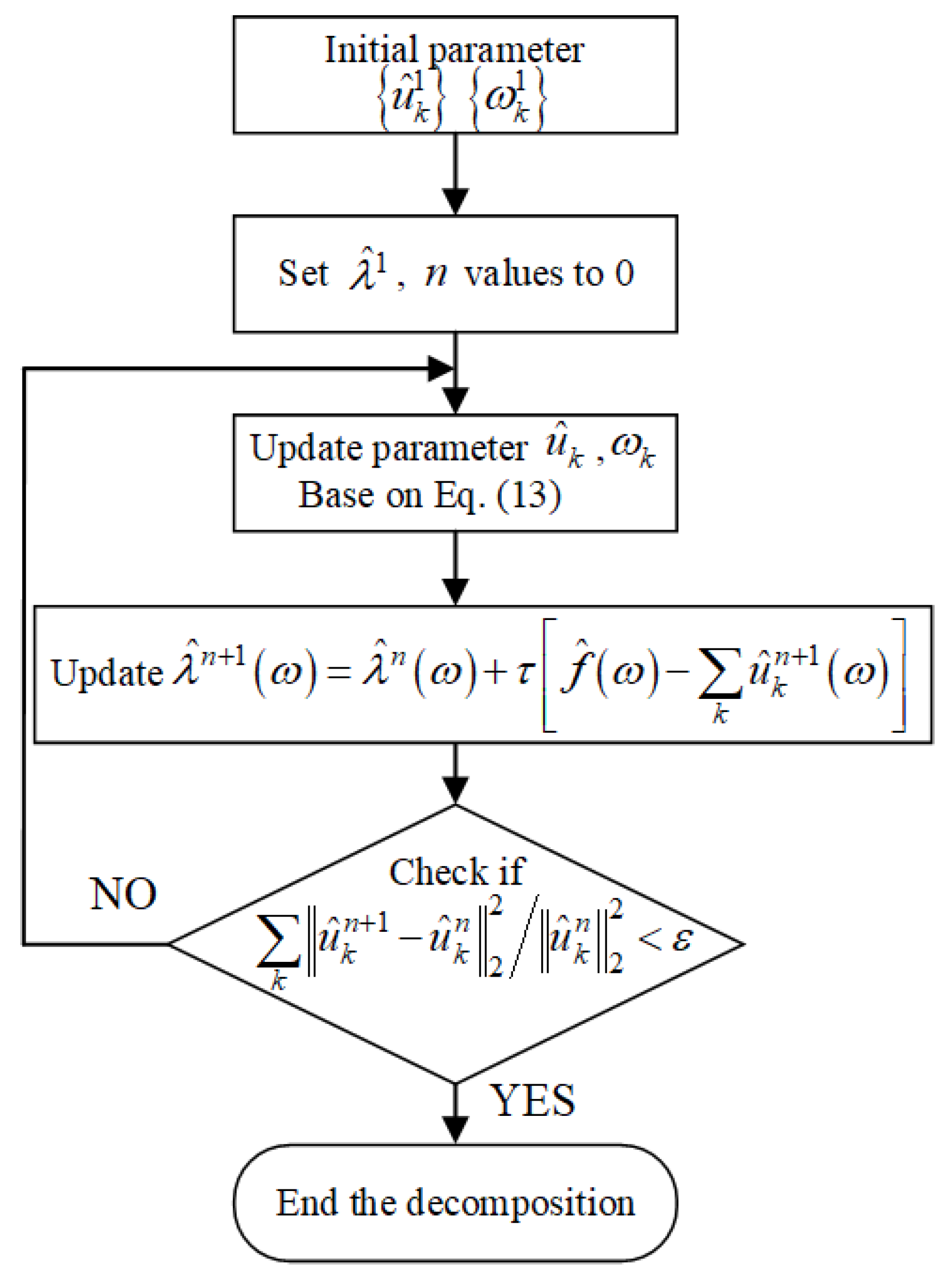
2.1. Variational Mode Decomposition

Different from EMD, VMD is an adaptive and non-recursive method that can analyze both nonstationary and nonlinear signals. The scope of VMD decomposes a signal into band-limited sub-signals by using a non-recursive calculation method. Each decomposed sub-signal has certain sparse properties in the frequency domain. Additionally, the decomposed sub-signal is defined as the mode as well as EMD. Moreover, each sub-signal is assumed to be concentrated around a corresponding frequency centre. Thus, the bandwidth of each sub-signal can be chosen by utilizing the H1 Gaussian smoothness for the transformed signal.

VMD first utilizes the Hilbert transform to convert each mode u_k into an analytical expression u_k⁺ in a single-sided spectral domain to obtain the bandwidth of each mode function:

$$u_k^{+}(t)=\left(\delta (t)+\frac{j}{\pi t}\right)\ast u_k(t)$$

(1)

After the Hilbert transformation, the frequency spectrum of each mode is shifted to the baseband and the corresponding estimated centre frequency ω_k is adjusted by using an exponential tuned term. Subsequently, the bandwidth is estimated according to the Gaussian smoothness of the demodulated signal by utilizing the squared L2-norm of the gradient [25]. Thus, the VMD process is realized by solving a constrained variational problem [26]:

$$\underset{\left\{u_k\right\},\left\{{\omega }_k\right\}}{\min }\left\{{\displaystyle \sum _{k=1}^K{\Vert \partial \left[\left(\delta (t)+\frac{j}{\pi t}\right)\ast u_k(t)\right]e^{-j{\omega }_{k}t}\Vert }_2^2}\right\},subjectto{\displaystyle \sum _{k=1}^K{u}_k(t)}=f(t)$$

(2)

where f(t) is the target signal, {u_k}: = {u₁, …, u_K} represents the set of the decomposed modes, and {ω_k}: = {ω₁, …, ω_K} represents the respective centre frequencies, respectively. Subsequently, the constraint optimization problem in Equation (2) can be converted into an unconstrained problem via a quadratic penalty term and Lagrangian multipliers, as below:

$$\mathcal{L}\left(\left\{u_k\right\},\left\{{\omega }_k\right\},\lambda \right)=\alpha {\displaystyle \sum _{k=1}^K{\Vert \partial \left[\left(\delta (t)+\frac{j}{\pi t}\right)\ast u_k(t)\right]e^{-j{\omega }_{k}t}\Vert }_2^2}+{\Vert f(t)-{\displaystyle \sum _{k=1}^K{u}_k(t)}\Vert }_2^2+\langle \lambda (t),f(t)-{\displaystyle \sum _{k=1}^K{u}_k(t)}\rangle$$

(3)

To solve the original minimization problem, the alternate direction method of multipliers (ADMM) is adopted to determine the saddle point of the augmented Lagrangian in a sequence of iterative suboptimizations. [21] summarizes the details of the VMD algorithm. By this process, all of the mode functions are obtained and updated by Wiener filtering to tune the centre frequency in the spectral domain:

$$\begin{array}{l}{\widehat{u}}_k^{n+1}(\omega )=\frac{\widehat{f}(\omega )-{\displaystyle {\sum }_{i<k}{\widehat{u}}_i^{n+1}(\omega )}-{\displaystyle {\sum }_{i>k}{\widehat{u}}_i^n(\omega )}+\frac{{\widehat{\lambda }}^n(\omega )}{2}}{1+2\alpha {(\omega -{\omega }_k^n)}^2}(\omega >0)\\ {\omega }_k^{n+1}=\frac{{\displaystyle {\int }_0^{\infty }\omega {\left|{\widehat{u}}_k^{n+1}(\omega )\right|}^{2}d\omega }}{{\displaystyle {\int }_0^{\infty }{\left|{\widehat{u}}_k^{n+1}(\omega )\right|}^{2}d\omega }}\end{array}$$

(4)

The centre frequency ω_kⁿ is calculated from the weighted centre of each mode in the spectral domain: the centre represents the frequency of the least squares linear regression of the instantaneous phase. Figure 1 presents the VMD algorithm as well as Appendix A.

2.2. Permutation Entropy

Entropy is a conventional approach to indicate the degree of uncertainty for a random system in the field of information theory. As entropy increases with the degree of randomness for an observed system, it can be utilized in a quantitative analysis for feature extraction in the field of PQD detection. Permutation entropy is one of most popular entropies in signal processing [22]. The temporal information of the monitored object is recognized according to permutation entropy by counting the ordinal patterns. Permutation entropy can estimate the complexity of a time-series after comparing the neighbouring values. By definition, permutation entropy is calculated by the time-series probability density function that is based on Shannon entropy. For a time domain series with a finite length of N, {x(t)} (t = 1, 2, …, N), a segment can be constructed by an m-order dimension. Each m-order segment is then sorted in an ascending sequence that is defined as permutation pattern π. The m-order segment X is defined in Equation (5) while considering the time delay α:

$$X_i^m=\left\{x\left(i+\alpha \left(j_1-1\right)\right),x\left(i+\alpha \left(j_2-1\right)\right),\cdots ,x\left(i+\alpha \left(j_m-1\right)\right)\right\}$$

(5)

From practical experience, the time lag α is selected as 1 and the value m is from 3 to 7. Hence, the number of m-order permutation patterns π is the factorial of m. The relative frequency of each permutation pattern π is calculated in Equation (6):

$$p\left(\pi \right)=\frac{H\left\{X_i^{m}hastype\pi ,i|1,2,\dots ,N-m+1\right\}}{N-m+1}$$

(6)

where H represents a number. Subsequently, permutation entropy PE(m) is calculated while using the probability density function p(π) for the relative frequency in Equation (7):

$$PE(m)=-{\displaystyle \sum _{i=1}^{m!}p\left({\pi }_i\right)\log \left(p\left({\pi }_i\right)\right)}$$

(7)

2.3. Fisher Score- Based Feature Selection Method

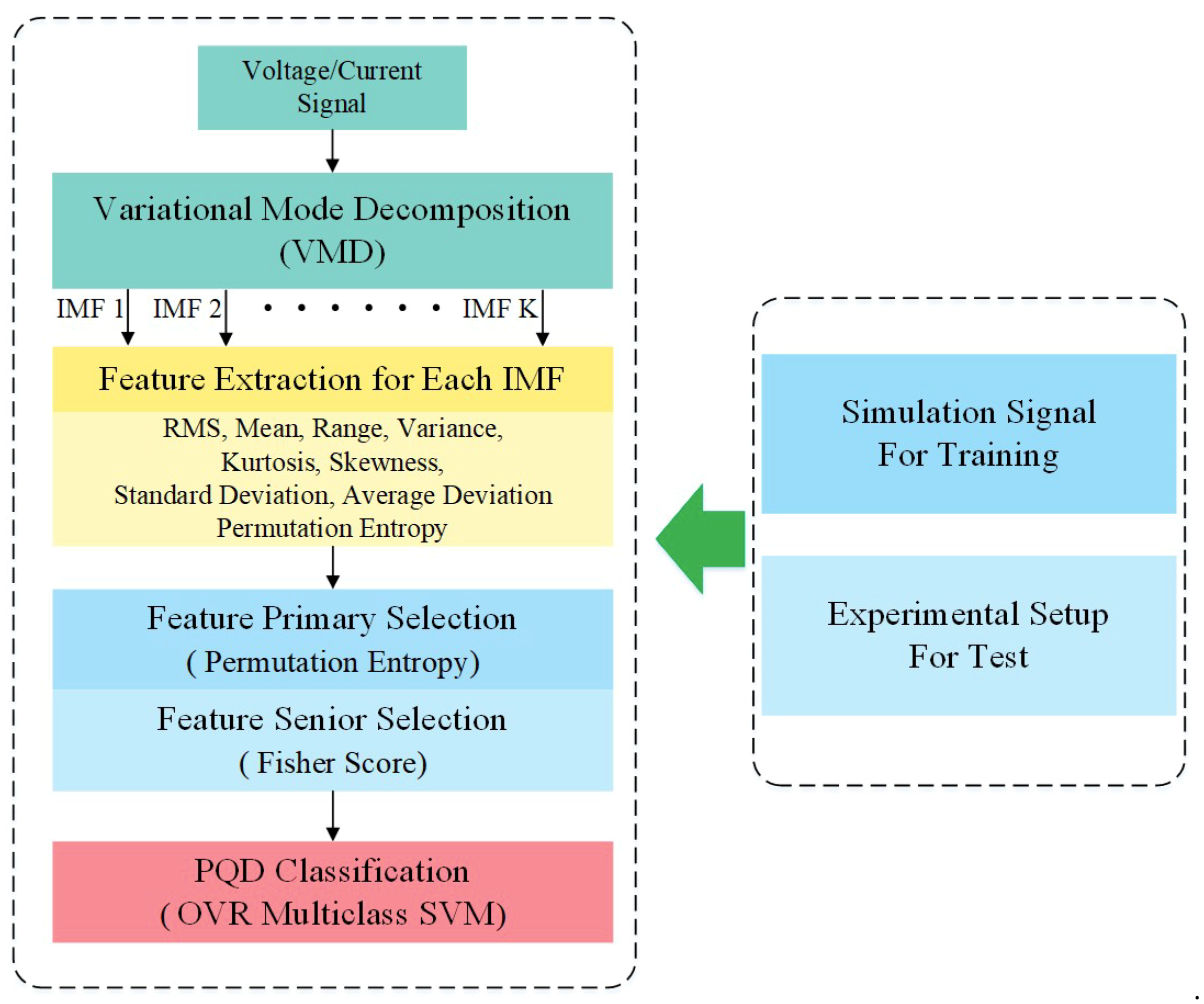
As mentioned above, a number of features can be extracted according to the behavior of the statistical method. However, the extracted features are not all useful for the classification, which might be redundant or irrelevant. It is essential to select the significant features and discard irrelevant features to improve the accuracy of the classification. Meanwhile, low dimensionality is beneficial to simultaneously reduce the computation burden and improve the efficiency of the classification algorithm. Various methods, such as Laplacian Score, Fisher score, ReliefF, Wilcoxon rank, and Gain Ratio, are valid for feature selection.

The Fisher score is one of the most popular algorithms for ranking the priority of features [27,28]. As a supervised algorithm, the Fisher score ranks extracted features by the Fisher criterion. In this method, the extracted features can be quantified in discriminative scores for different classes. For instance, the data set {f_ik(1), f_ik (2), …f_ik (N)} is defined as the kth feature in the ith class. First, the mean value u_ik and standard deviation σ²_ik of the kth feature are calculated, as follows:

$$\begin{array}{l}{u}_{ik}=\frac{1}{N}{\displaystyle \sum _{p=1}^{N_i}{f}_{ik}}\\ {\sigma }_{ik}^2=\frac{1}{N}{\displaystyle \sum _{p=1}^{N_i}{\left(f_{ik}-u_{ik}\right)}^2}\end{array}$$

(8)

Afterwards, the Fisher score value FS_ij between the ith and the jth class can be quantified, as follows:

$$F{S}_{ij}^{(k)}=\frac{{\displaystyle \sum _{k=1}^C{\left(f_{ij}^k-u_i^k\right)}^2}}{{\displaystyle \sum _{k=1}^C{\displaystyle \sum _{yi\in k}{\left(f_{ij}^k-u_i^k\right)}^2}}}$$

(9)

As observed from the Fisher score expression, a large value represents a highly relevant correlation of the kth feature between the ith and the jth classes. A larger Fisher score indicates that the corresponding feature reveals more relevant distinction between the classes. The feature has a high priority to be chosen for the training model.

3. Proposed Method

Figure 2 presents the flowchart of the proposed method. The main scheme is implemented in four steps: PQD generation in a computer simulation, feature extraction, optimization of feature selection, and pattern recognition. In this paper, the proposed algorithm is designed to classify 13 classes of different signals, which are generated as a pure sine signal, sag, swell, interrupt, harmonics, sag with harmonics, swell with harmonics, interrupt with harmonics, flicker, oscillatory transient, impulsive transient, periodic notch, and spike. Second, by utilizing VMD to decompose the target signal into several IMFs, the feature vector is extracted in the statistical analysis method. Third, permutation entropy is imported to filter the invalid IMFs. Subsequently, the Fisher score is adopted to eliminate the redundant features to optimize feature selection. Finally, the classifier is realized by SVM to recognize different PQD patterns.

The training data is generated from computer simulation with the 13 classes mentioned above. The dataset size of each class is 1000. After training, several analysis methods, such as confusion matrix and receiver operating characteristic curve, are imported to evaluate the performance of the training model, which is presented in Section 4.4. In another word, the artificial dataset of the simulation signals is utilized for the training and developed set. Additionally, the trained model will be tested on the real experimental setup to verify the effectiveness of the classifier, which is presented in Section 4.5.

As specific implementation, the data generation and preprocessing, including the VMD algorithm, is realized on the Python script in the training stage. Subsequently, the public feature extraction library, LibXtract, is integrated with the console application to extract features. Afterwards, the feature heuristic selection and classifier model is trained on the server setup in Anaconda Python. In the training stage, the fault simulator system and the data acquisition system are both integrated on the LabVIEW environment. In particular, the communication is realized by the data-logging and supervisory control (DSC) packet. Additionally, the DAQmx driver packet realizes the data acquisition system. The experimental voltage/current data in time domain is obtained and saved as csv format in files. As an alternative method, the proposed algorithm can be realized on other platforms, such as C++ and Matlab.

3.1. Computer Simulation of PQDs

In this work, a set of signals for training is artificially obtained through computer models. The artificial PQD signals consist of 10 single types, including pure a sine signal, sag, swell, interrupt, harmonics, flicker, oscillatory transient, impulsive transient, periodic notch, and spike. The multiple types consist of sag with harmonics, swell with harmonics, and interrupt with harmonics. The definition of the PQD signals with the parameter variations is based on the IEEE-1159 standard [29], as presented in

Table 1. Mathematical model of the power quality disturbances.

Label	PQD Type	Mathematical Mode	Parameters
C1	Pure Sine	$y\left(t\right)=A\sin \left(\omega t\right)$	$\begin{array}{l}A=1\\ \omega =2\pi *50\end{array}$
C2	Sag	$y\left(t\right)=A\left[1-\alpha \left(u\left(t-t_1\right)-u\left(t-t_2\right)\right)\right]\sin \left(\omega t\right)$	$\begin{array}{l}0.1\le \alpha \le 0.9\\ T\le t_2-t_1\le 9T\end{array}$
C3	Swell	$y\left(t\right)=A\left[1+\alpha \left(u\left(t-t_1\right)-u\left(t-t_2\right)\right)\right]\sin \left(\omega t\right)$	$\begin{array}{l}0.1\le \alpha \le 0.8\\ T\le t_2-t_1\le 9T\end{array}$
C4	Interrupt	$y\left(t\right)=A\left[1-\alpha \left(u\left(t-t_1\right)-u\left(t-t_2\right)\right)\right]\sin \left(\omega t\right)$	$\begin{array}{l}0.9\le \alpha \le 1;\\ T\le t_2-t_1\le 9T\end{array}$
C5	Harmonics	$y\left(t\right)=A\left[{\alpha }_1\sin \left(\omega t\right)+{\alpha }_3\sin \left(3\omega t\right)+{\alpha }_5\sin \left(5\omega t\right)+{\alpha }_7\sin \left(7\omega t\right)\right]$	$\begin{array}{l}0.05\le {\alpha }_3,{\alpha }_5,{\alpha }_7\le 0.15\\ {\displaystyle \sum {\alpha }_i^2}=1\end{array}$
C6	Flicker	$y\left(t\right)=A\left[1+{\alpha }_f\sin \left(\beta \omega t\right)\right]\sin \left(\omega t\right)$	$\begin{array}{l}0.1\le \alpha \le 0.2\\ 5\le \beta \le 20Hz\end{array}$
C7	Oscillatory transient	$y\left(t\right)=A\left[\sin \left(\omega t\right)+{\alpha }^{-c\left(t-t_1\right)/\tau }\sin \left({\omega }_n\left(t-t_1\right)t\right)\left(u\left(t_1\right)-u\left(t_2\right)\right)\right]$	$\begin{array}{l}0.1\le \alpha \le 0.8\\ 0.5T\le t_2-t_1\le 3T\\ 8\mathrm{ms}\le \tau \le 40\mathrm{ms}\\ 300\le f_n\le 900Hz\end{array}$
C8	Impulsive transient	$y\left(t\right)=A\left[1-\alpha \left(u\left(t-t_1\right)-u\left(t-t_2\right)\right)\right]\sin \left(\omega t\right)$	$\begin{array}{l}0\le \alpha \le 0.414\\ 0.05T\le t_2-t_1\le 0.1T\end{array}$
C9	Periodic notch	$\begin{array}{l}y\left(t\right)=\sin \left(\omega t\right)-\mathrm{sign}\left(\sin \left(\omega t\right)\right)\\ \times \left\{{\displaystyle \sum _{n=0}^{9}K\times \left[u\left(t-\left(t_1-0.02n\right)\right)-u\left(t-\left(t_2-0.02n\right)\right)\right]}\right\}\end{array}$	$\begin{array}{l}0\le t_1,t_2\le 0.5T\\ 0.01T\le t_2-t_1\le 0.05T\\ 0.1\le K\le 0.4\end{array}$
C10	Spike	$\begin{array}{l}y\left(t\right)=\sin \left(\omega t\right)+\mathrm{sign}\left(\sin \left(\omega t\right)\right)\\ \times \left\{{\displaystyle \sum _{n=0}^{9}K\times \left[u\left(t-\left(t_1-0.02n\right)\right)-u\left(t-\left(t_2-0.02n\right)\right)\right]}\right\}\end{array}$	$\begin{array}{l}0\le t_1,t_2\le 0.5T\\ 0.01T\le t_2-t_1\le 0.05T\\ 0.1\le K\le 0.4\end{array}$
C11	Sag with harmonics	$y\left(t\right)=A\left[1-\alpha \left(u\left(t-t_1\right)-u\left(t-t_2\right)\right)\right]\left[{\alpha }_1\sin \left(\omega t\right)+{\alpha }_3\sin \left(3\omega t\right)+{\alpha }_5\sin \left(5\omega t\right)\right]$	$\begin{array}{l}0.1\le \alpha \le 0.9;\\ T\le t_2-t_1\le 9T\\ 0.05\le {\alpha }_3,{\alpha }_5,{\alpha }_7\le 0.15;\\ {\displaystyle \sum {\alpha }_i^2}=1\end{array}$
C12	Swell with harmonics	$y\left(t\right)=A\left[1+\alpha \left(u\left(t-t_1\right)-u\left(t-t_2\right)\right)\right]\left[{\alpha }_1\sin \left(\omega t\right)+{\alpha }_3\sin \left(3\omega t\right)+{\alpha }_5\sin \left(5\omega t\right)\right]$	$\begin{array}{l}0.1\le \alpha \le 0.9\\ T\le t_2-t_1\le 9T\\ 0.05\le {\alpha }_3,{\alpha }_5,{\alpha }_7\le 0.15\\ {\displaystyle \sum {\alpha }_i^2}=1\end{array}$
C13	Interrupt with harmonics	$y\left(t\right)=A\left[1-\alpha \left(u\left(t-t_1\right)-u\left(t-t_2\right)\right)\right]\left[{\alpha }_1\sin \left(\omega t\right)+{\alpha }_3\sin \left(3\omega t\right)+{\alpha }_5\sin \left(5\omega t\right)\right]$	$\begin{array}{l}0.9\le \alpha \le 1\\ 0.05\le {\alpha }_3,{\alpha }_5,{\alpha }_7\le 0.15\\ {\displaystyle \sum {\alpha }_i^2}=1\end{array}$

. Waveform signals with 10 cycles are generated for 2000 points at a 10 kHz sampling frequency. The parameter A represents the normalized amplitude at a constant value. The parameter α represents the intensity levels of the sag, swell, and interruption. The expression u(t) denotes the time step function.

In this work, all of the studied cases are based on pure normal-class sinusoidal signals that can vary their amplitude within 10% of their ideal magnitude. Additionally, the probability of a signal containing noise must be considered. Therefore, the simulated signal is coupled with Gaussian noise contamination at different signal-to-noise ratios (SNRs) in this paper. The SNR is defined, as follows, where P_s represents the original signal power and P_n represents the noise power correspondingly.

$$SNR=10*\log \left(\frac{P_s}{P_n}\right)$$

(10)

3.2. PQD Feature Extraction

For the recognition of different PQD patterns, it is essential to utilize a classifier to analyze the signal that is obtained from the voltage or current sensors. However, it is difficult to identify the time-series signal directly for common classification methods. As feature extraction plays an important role in the pattern recognition schemes, VMD is utilized to decompose the obtained signal into several IMFs for potential feature extraction in this paper. The sub-mode decomposed by VMD contains a specific spectrum, which can accurately trace the signal changes of the power quality. Thus, signal decomposition can effectively eliminate the impact of noise and separate the useful components in high level modes. As mentioned above, the decomposition results depend on the mode number, which is defined as K. When considering the harmonic components that exist in the PQD signal, the value of K is selected as 5. Additionally, parameter α of the data-fidelity constraint is selected as 2500 based on the experimental trial. Subsequently, by generating artificial PQD signals, the IMF is decomposed by VMD. After the decomposition, the statistical features are calculated and extracted from each mode in the time domain.

Table 2. Statistical parameters for feature extraction.

No.	Statistical Feature	Expression
1	RMS	$RMS=\sqrt{\frac{1}{K}{\displaystyle \sum _{k=1}^K{\left[x(k)\right]}^2}}$
2	Mean	$\mu ={\displaystyle \sum _{k=1}^K\left[x(k)\right]}/K$
3	Standard Deviation	$\sigma =\sqrt{{\displaystyle \sum _{k=1}^K{\left[x(k)-\overline{x}\right]}^2}/\left(K-1\right)}$
4	Variance	$\mathrm{var}={\displaystyle \sum _{k=1}^K{\left[x(k)-\overline{x}\right]}^2}/K$
5	Range	$range=\max \left(x(k)\right)-\min \left(x(k)\right)$
6	Kurtosis	$KT={\displaystyle {\sum }_{k=1}^K{\left[\left(x(k)-\overline{x}\right)/\sigma \right]}^4/K}$
7	Skewness	$SK={\displaystyle {\sum }_{k=1}^K{\left[\left(x(k)-\overline{x}\right)/\sigma \right]}^3/K}$
8	Average Deviation	$\overline{\sigma }={\displaystyle {\sum }_{k=1}^K\left|x(k)-\overline{x}\right|/K}$
9	Permutation Entropy	$PE=-{\displaystyle \sum _{i=1}^{m!}p\left({\pi }_i\right)\log \left(p\left({\pi }_i\right)\right)}$

marks and lists all of the features and the corresponding labels.

With the proposed feature extraction method, the PQD signals are decomposed into five IMFs. Subsequently, the statistical feature vectors are given as the following equations, where F₁, F₂, …, F₉ represent the feature vectors of RMS, standard deviation, variance, range, skewness, kurtosis, mean, average deviation, and permutation entropy, respectively.

$$\begin{array}{l}{F}_1=\left[RMS1RMS2RMS3RMS4RMS5\right]\\ F_2=\left[{\mu }_1{\mu }_2{\mu }_3{\mu }_4{\mu }_5\right]\\ F_3=\left[{\sigma }_1{\sigma }_2{\sigma }_3{\sigma }_4{\sigma }_5\right]\\ F_4=\left[{\mathrm{var}}_1{\mathrm{var}}_2{\mathrm{var}}_3{\mathrm{var}}_4{\mathrm{var}}_5\right]\\ F_5=\left[rang{e}_{1}rang{e}_{2}rang{e}_{3}rang{e}_{4}rang{e}_5\right]\\ F_6=\left[K{T}_{1}K{T}_{2}K{T}_{3}K{T}_{4}K{T}_5\right]\\ F_7=\left[S{K}_{1}S{K}_{2}S{K}_{3}S{K}_{4}S{K}_5\right]\\ F_8=\left[{\overline{\sigma }}_1{\overline{\sigma }}_2{\overline{\sigma }}_3{\overline{\sigma }}_4{\overline{\sigma }}_5\right]\\ F_9=\left[P{E}_{1}P{E}_{2}P{E}_{3}P{E}_{4}P{E}_5\right]\end{array}$$

(11)

The data must be normalized between 0 and 1 by using the min-max normalization method in Equation (12), where Z_i is the normalized data, F_max is the maximum data of the vector, and F_min is the minimum data, respectively, since the elements of the extracted feature sets have different units.

$$Z_{\mathrm{i}}=\frac{F_i-F_{\min }}{F_{\max }-F_{\min }}$$

(12)

After normalization, the feature set F is obtained while using Equation (13).

$$F=\left[F_1{F}_2{F}_3{F}_4{F}_5{F}_6{F}_7{F}_8{F}_9\right]$$

(13)

3.3. PQD Feature Heuristic Selection

The original feature vectors in high dimensions contain not only useful information, but also redundant messages. As a result, the original high dimensional feature vectors would lead to the waste of computer resources and a decrease in accuracy. In this paper, a two-stage heuristic feature selection algorithm is adopted to filter relevant features for the classification of PQDs. When considering the function of the VMD method, some decomposed IMFs may be the separated noise, which contains little useful information. As a result, it is obligatory to remove these feature vectors extracted from the useless IMFs. Further, permutation entropy is imported by estimating the time-series complexity of the obtained IMF to select IMFs. In this work, a hard threshold of permutation entropy is computed to select valid IMFs, which is set as 0.6. In other words, if the permutation entropy of the IMF is larger than 0.6, the decomposed IMF is treated as chaotic with less useful information [30].

In the second stage, the Fisher score is adopted to filter the relevant features. As described above, if the feature is highly relevant, the corresponding Fisher score is relatively large. Hence, the classification accuracy would achieve perfection. On the contrary, if the feature shows irrelevance for the classification result, the Fisher score is near zero. In this circumstance, the classifier would have poor performance. In addition, one point should be noted: the threshold selection of the Fisher’s score is very important. In this study, the threshold value of the Fisher score is set as 0.25 and Section 4.3 discusses the reason of the threshold selection.

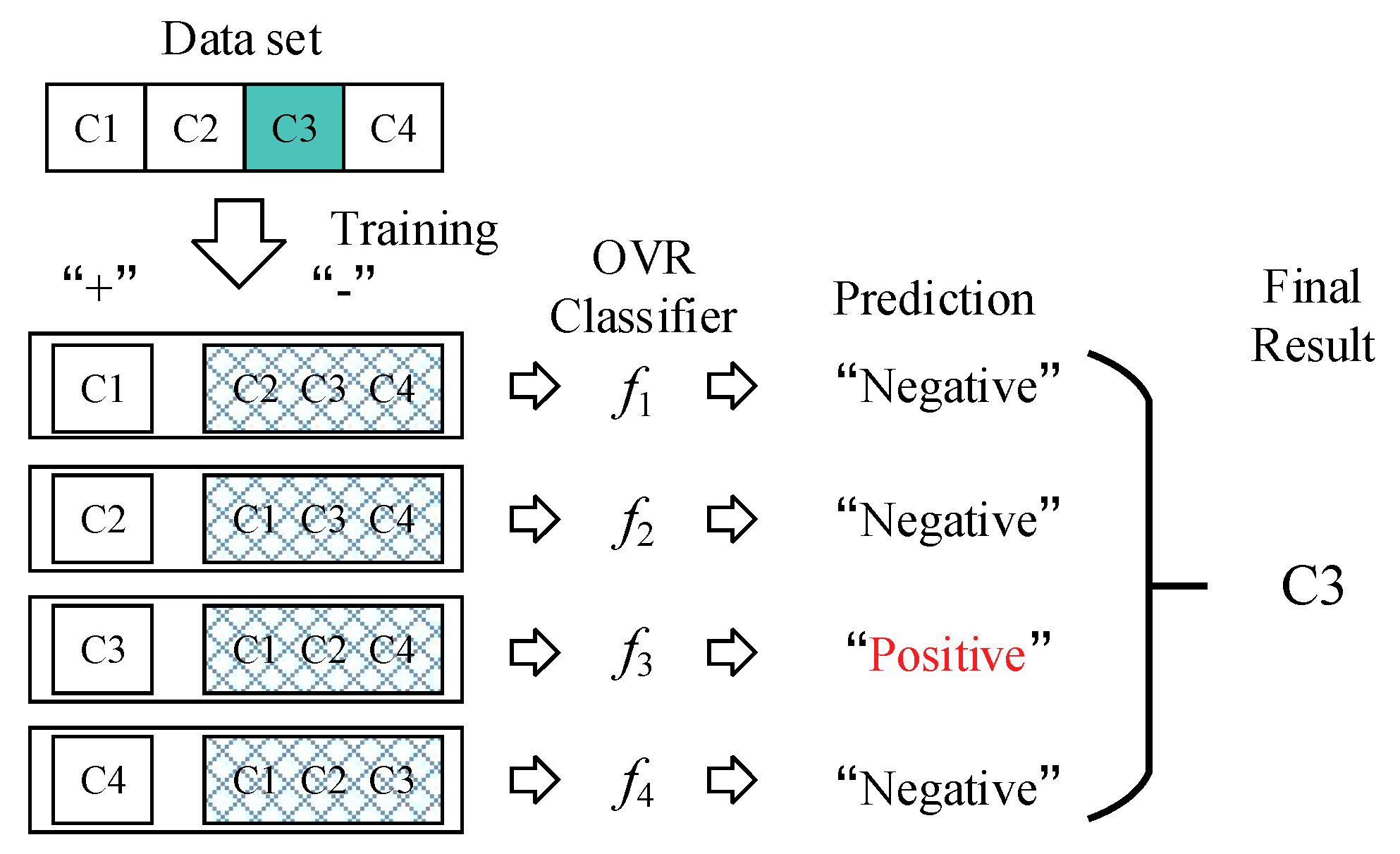
3.4. Multiclass Classification for PQDs

After feature selection, a support vector machine (SVM) is utilized as the classifier to identify the pattern of PQDs. It is essential to adjust the strategies that are used for multiclass classification since the original SVM was designed for binary classification. When compared with binary classification problems, multi classification is more complex and it contains large datasets [31]. In this paper, the strategy “one-versus-rest” (OVR) is adopted to expand the SVM for multiclass classification. For an N-class problem, N hyperplanes are generated for N classes. When generating the ith hyperplane of the ith class, SVM treats the ith class as the positive case. Meanwhile, the rest are treated as a negative class. During the classifying process, all of the samples are required in each quadratic programming problem. The new sample is assigned to the corresponding class by calculating the closest distant to the hyperplane.

Figure 3 gives an example of the OVR strategy. When considering a data set with four classes marked C1, C2, C3, and C4, the OVR strategy treats each class as the positive example and the rest as negative examples. Therefore, four classifiers will be trained to give the predicted result. If there is only one classifier like f₃ predicts the sample as positive, the final result is determined. Otherwise, it is usually referred the forecast confidence given by each classifier. Subsequently, choose the maximum value as the final result.

In this paper, the radial basis function (RBF) is chosen as the kernel function of the SVM, because the selected features are nonlinear and the quadratic programming problem is not linearly separable. By choosing a nonlinear kernel, the SVM model will build a nonlinear classification boundary. Furthermore, the penalty parameter C and the adjustable parameter γ in the SVM with an RBF kernel are optimized by conducting the grid search algorithm. In particular, C is the penalty coefficient, which is representative of the tolerance for error. The higher C is, the less error is tolerated, which makes the classifier model over-fit. The smaller C is, the easier it is to under-fit. If C is too large or too small, the generalization ability of the classifier would be poor. Parameter γ comes with the RBF function when it is selected as kernel. It implicitly determines the distribution of data after mapping to the new eigenspace. The larger the gamma is, the less the support vector is, the smaller the gamma value is, and the more the support vector is.

4. Experimental Results and Discussion

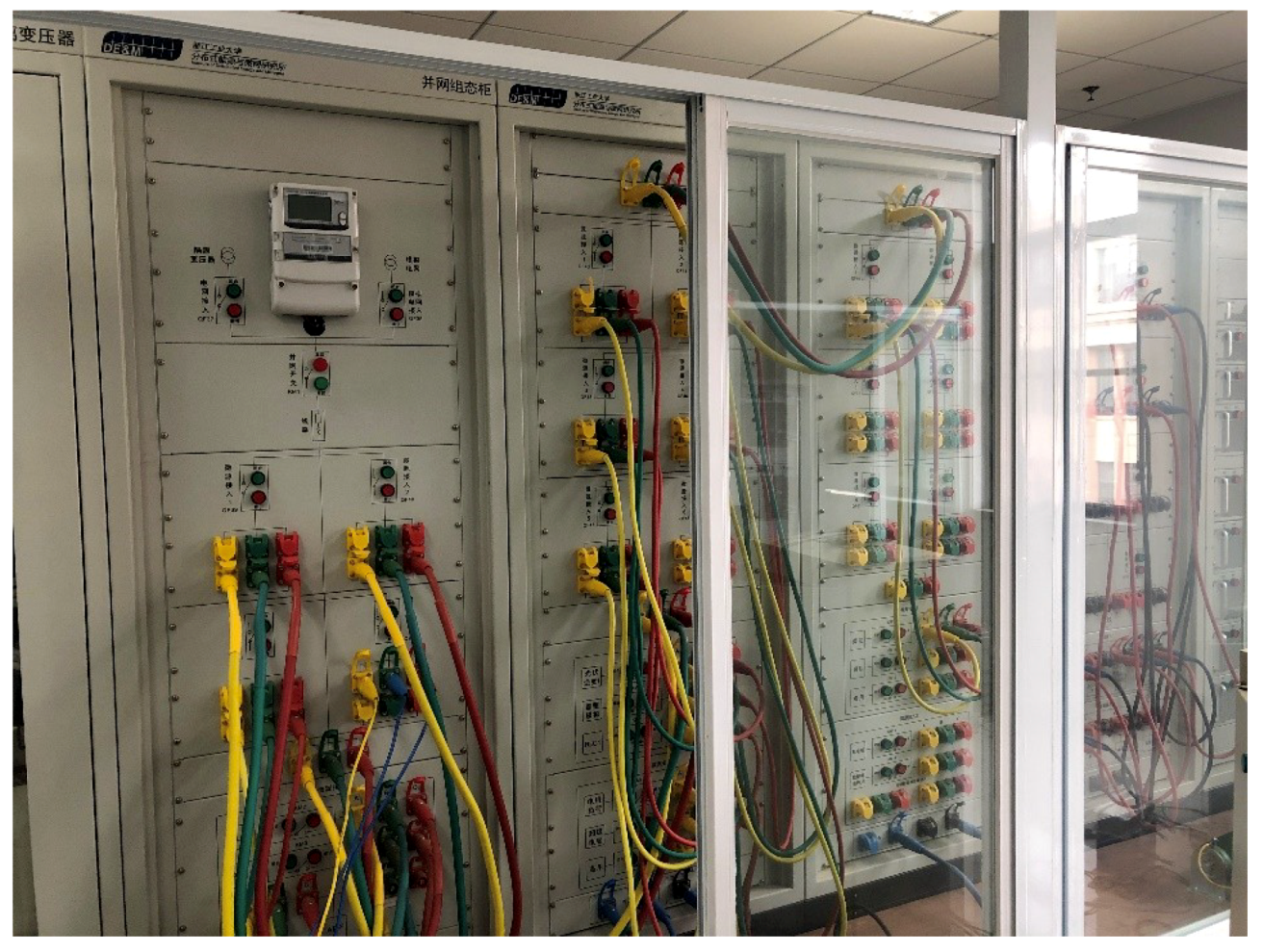
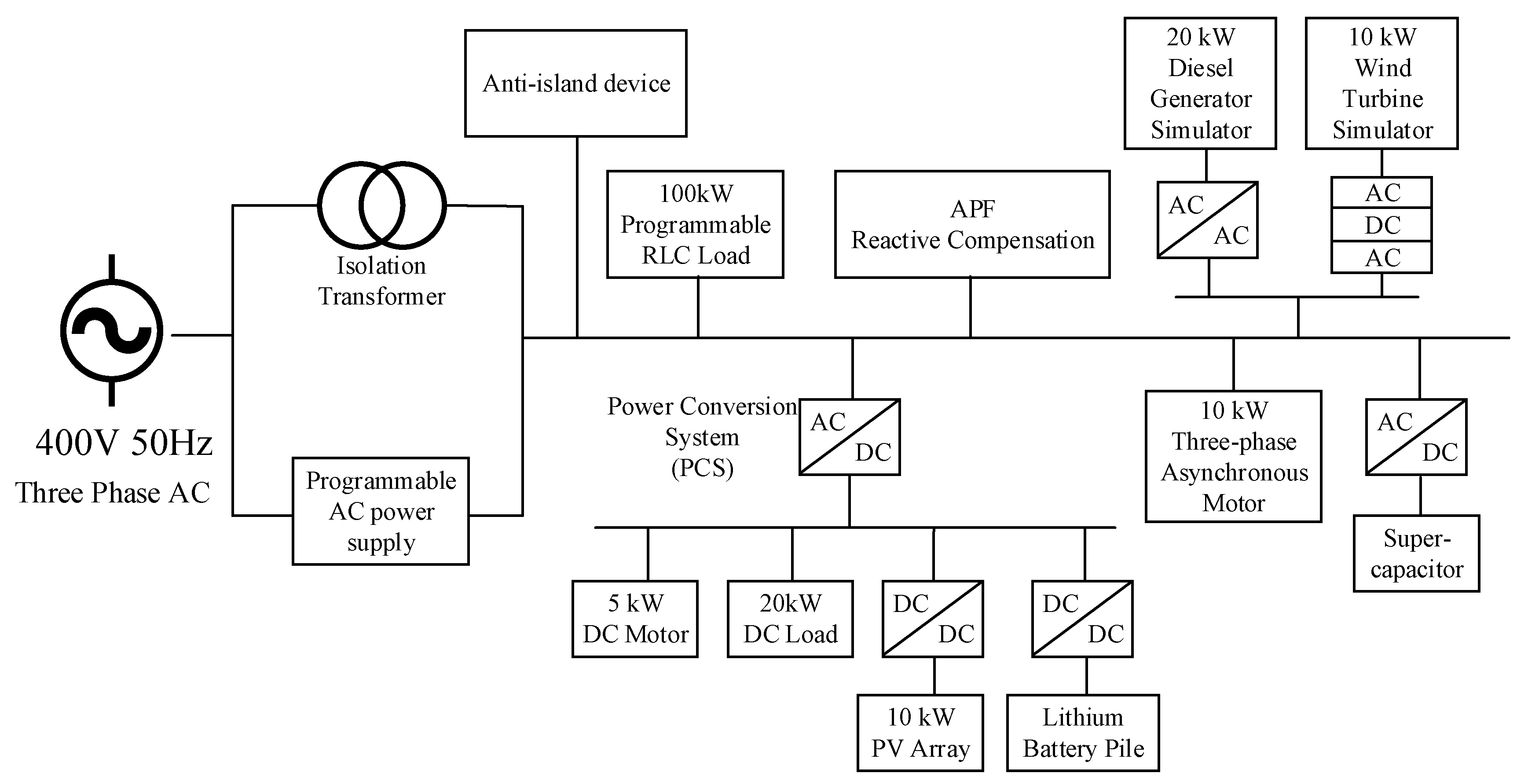
4.1. Experimental Setup

A microgrid platform is built in the laboratory environment to verify the proposed method, as shown in Figure 4 and Figure 5. The microgrid platform is designed in a double layer structure with a flexible topology that contains flexible line connection, distributed generations like PV array and wind turbine, line impedance simulators, including resistance, and inductive and capacitive loads (100 kW RLC Load). To be specific, the distributed generations consist of centralized inverters for the photovoltaic roof, microinverters for the photovoltaic roof, a photovoltaic simulator, a diesel generator simulator, and a wind turbine simulator. Moreover, the load of the microgrid platform consists of lighting systems, an induction motor, charging piles for electric vehicles, and a 100 kW programmable PLC load. The microgrid platform is designed to operate at 400 V three phases with 50 Hz. Two sub-microgrid layers are coupled with bidirectional converters, which allow for the electrical energy to be transmitted in bidirectional flows. These sub-microgrid layers are connected to the bulk power system by deploying the three phases AC bus. Moreover, the microgrid platform is able to simulate different line faults to recur by utilizing the line impedance simulator under the logical program control.

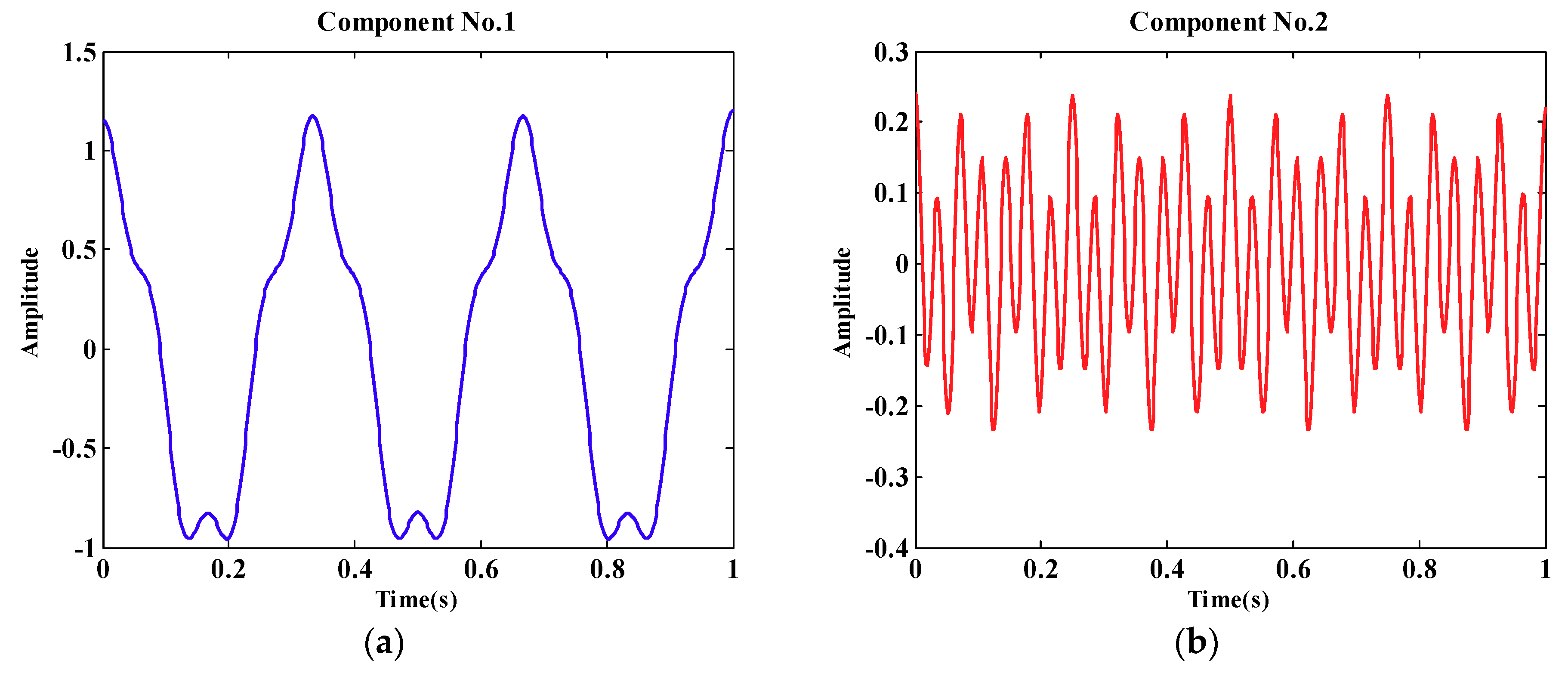
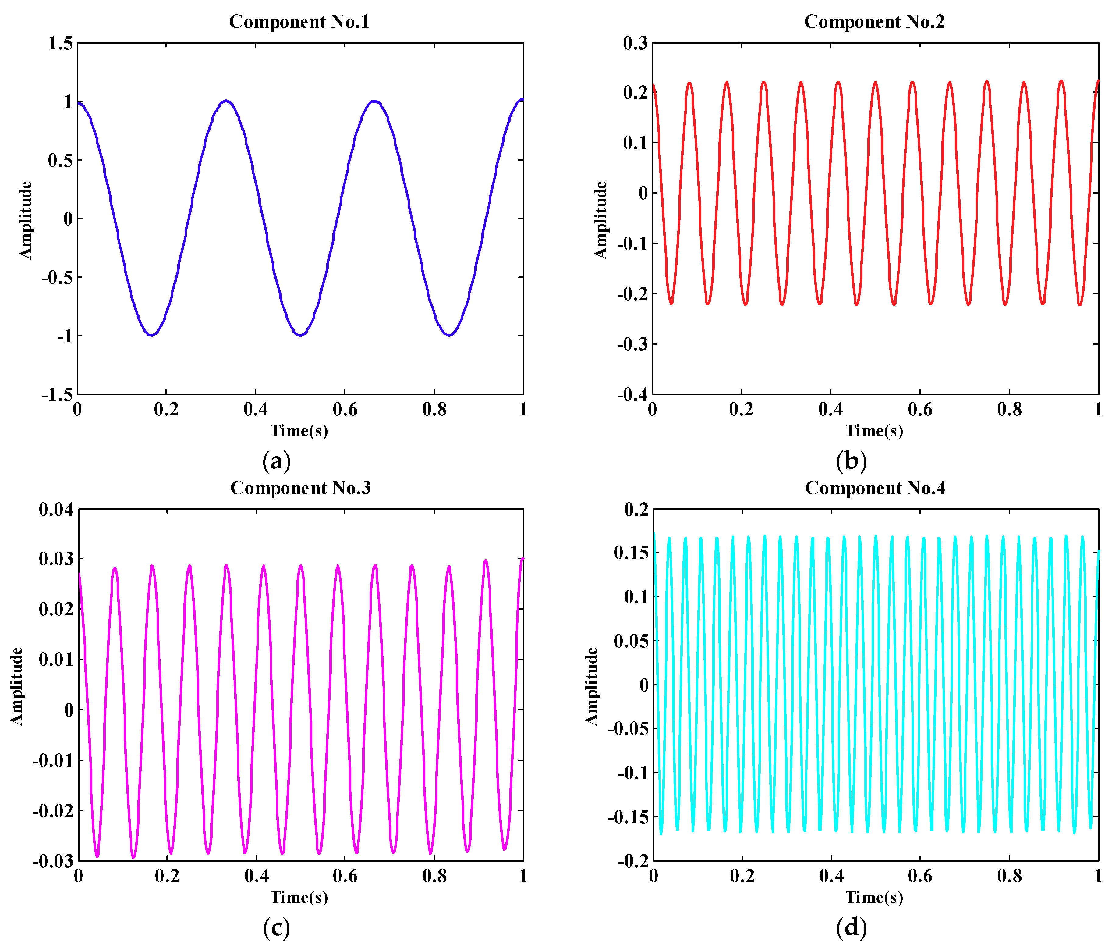
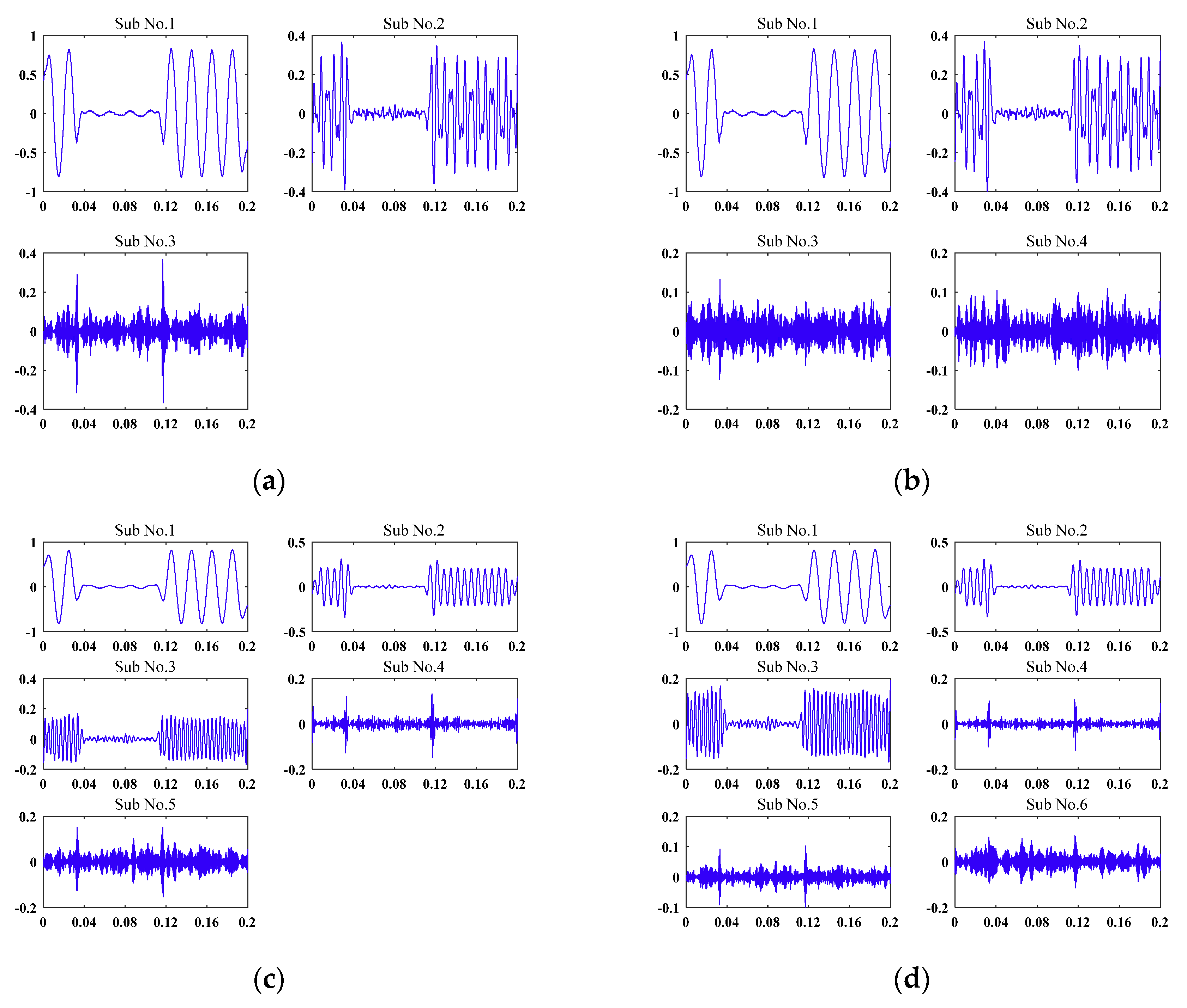
4.2. PQD Signal Decomposition and Detection

An artificial signal that represents an interruption with harmonics will be discussed, as follows, in order to verify the effectiveness of VMD. Figure 6 shows the PQD type of the interruption with third and fifth harmonics in the time series. As seen, the electric power is interrupted from 0.035 s to 0.117 s. Meanwhile, the obtained signal is contaminated with the third and fifth harmonics. Additionally, white noise is added with 25 dB SNR to represent the real signal.

Figure 7 presents the different decomposition result of VMD, and Figure 7a–d represent the decomposed number K = 3, 4, 5 and 6, respectively. When K = 3 in Figure 7a, it appears that the PQD signal is under-decomposed. Although the fundamental component is obtained in the first IMF, the third and fifth harmonics mix in the second IMF. Figure 7b shows the same result. When K = 5 in Figure 7c, the first three IMFs are decomposed as fundamental components, the third and fifth harmonics, effectively. Interestingly, the fourth IMF presents two mutation pulses for detecting the start and the end of the PQD. By setting an appropriate threshold, the start and the end of the PQD can be easily detected and implemented on the hardware with less computational cost. Meanwhile, Figure 7d also shows a similar result when K = 6, which reveals that the PQD signal is over-decomposed, because the other two IMFs share the noise component. Nevertheless, this situation is less harmful than the under-decomposed situation, since feature selection in the next step will help to filter redundant IMFs. Moreover, from Figure 7c, it is apparent that the first four IMFs carry valid information and the remaining IMFs are invalid. Therefore, it is obligatory to consider these four IMFs for feature extraction. Meanwhile, the permutation entropy of each IMF is 0.231, 0.357, 0.442, 0.553, and 0.689, which verifies the observation results.

Additionally, as referred to in Ref. [24], the wavelet packet decomposition (WPD) is imported for comparison. Figure 8a,b present the decomposition result by WPD when the decomposition level is 2 and 3, respectively. In Figure 8a, since the decomposition level is 2, the corresponding wavelet node is 4, which reveals that WPD can only filter noise, but the first node still retains the main component of the original signal. Though the number of the wavelet nodes increases to 8, it still reveals a similar result in Figure 8b. By contrast, VMD performs better, even if the decomposed number K is not suitable for decomposition. The reason for this phenomenon is that each node of the wavelet packet can be approximately treated as a band-pass filter at the specific frequency range. As mentioned in Section 3.1, the sampling frequency is selected as 10 kHz. For the two levels of WPD that are shown in Figure 8a, the band width of each node is approximately 1.25 kHz. Meanwhile, for the three levels of WPD that are shown in Figure 8b, the band width of each node is approximately 0.625 kHz. However, the PQD signal is defined as the interruption of the third and fifth harmonics, where sinusoidal components with frequencies of 50 Hz, 150 Hz, and 250 Hz exist. Hence, all of these components are retained and mixed in the first node, so the WPD does not seem to work effectively. Based on the decomposition result, VMD is adaptive and robust for PQD signal decomposition, especially for recursive calculation and mode mixing problems.

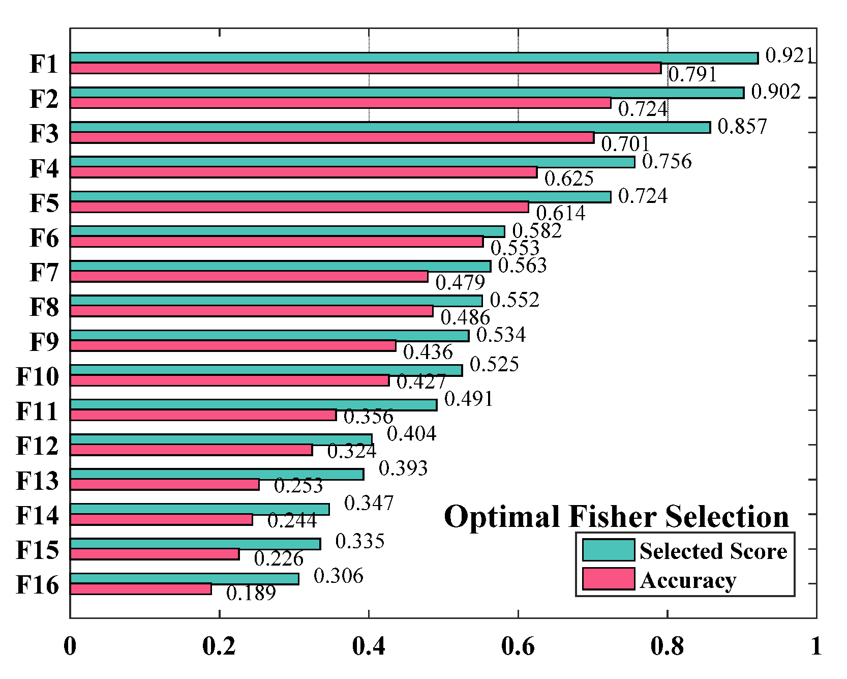
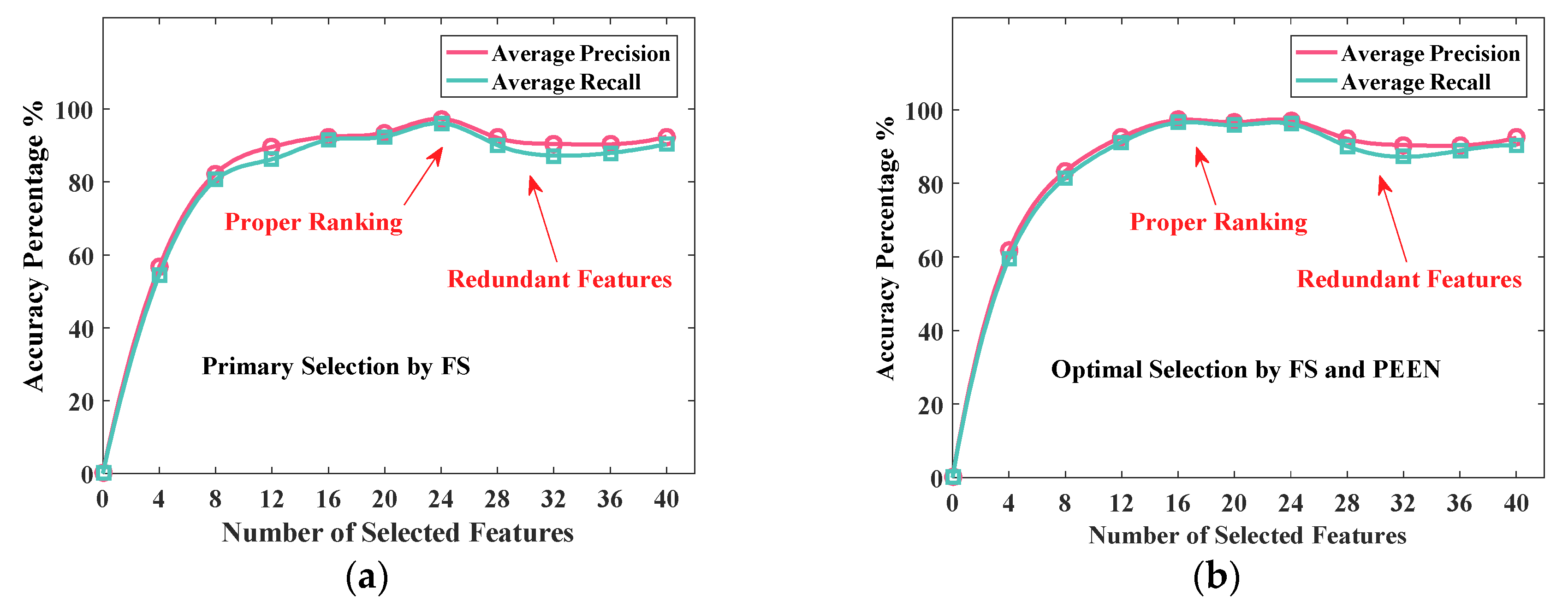
4.3. Feature Selection Analysis

The Fisher score with permutation entropy, which is described in Section 3.3, is utilized to filter redundant features as a feature heuristic selection method. Specifically, the embedded dimension parameter of permutation entropy is set to 6. Based on the experimental trial, the time delay parameter of permutation entropy is set to 1. The hard threshold of permutation entropy is set to 0.6. Figure 9 presents the correlation of the top 16 selected features, which represent the IMF2 RMS, IMF2 standard deviation, IMF2 variance, IMF2 average deviation, IMF2 kurtosis, IMF2 skewness, IMF2 range, IMF2 permutation entropy, IMF1 permutation entropy, IMF1 variance, IMF1 standard deviation, IMF1 RMS, IMF1 average deviation, IMF1 kurtosis, IMF1 range, and IMF4 permutation entropy. As shown, each feature is imported into the training dataset to determine the classification accuracy, with the aim of showing the effectiveness of the feature selection method. The experiments are conducted 50 times to avoid errors and stochastic disturbances. Subsequently, the accuracy results are generated by averaging the calculations. If the feature is irrelevant to the target class, the corresponding Fisher’s score is nearly zero. Hence, the average accuracy of the classification would be poor. Conversely, if the feature is highly relevant, the corresponding Fisher score is relatively large. Thus, the classifier that is constructed by relevant features would achieve perfect accuracy. Moreover, the threshold value of the selected feature is very important. Threshold selection is discussed in the following paragraph.

In this case, the SVM classifier is adopted to focus on the effects of the selected features. To be specific, the sample data sets are partitioned into 10 equal folds, and the tests were performed in 10 iterations. The number of each test instance is 1000. For the SVM classifier, the cost values C and γ of the SVM model are set to 100 and 0.02, respectively, and the linear kernel is selected as the kernel function. The classification threshold is set to 0.5. For each PQD class, the data sets were split into the training data sets and the test data sets. The ratio of the samples for the training and test is 4:1.

Two feature ranking methods, Fisher’s score only and Fisher’s score with the permutation algorithm, were used for feature selection for comparison. Figure 10a,b show the precision and recalls results by extracting different features according to the Fisher’s score only and Fisher’s score with the permutation algorithm, respectively. The average precision and average recall ratio reached 96.5% when the top 24 ranked features were selected by the Fisher’s scoring algorithm. Similarly, the average precision and the average recall ratio according to the Fisher’s score with the permutation algorithm achieved 97.6% when the SVM classifier was trained by feeding the 16 top-ranked features. However, the SVM classifier that was trained by the Fisher’s score with the permutation selection algorithm showed better performance. Moreover, it cost less dimensions for feature vectors.

Interestingly, as observed from the average precision and the average recall ratio, the accuracy was initially increased with the increased number of top-ranked features, because the decision boundary of the SVM hyperplane is more clearly separated by increasing the relevant feature vectors. However, once the feature dimension reached the proper ranking feature point, the performance of the classifier continued to decrease due to redundant features. After a decrease, the average precision and average recall ratio increased again, because the SVM imported the slack variable and the penalty factor to construct the decision boundary in soft intervals, which improved the robustness and generalization of the classifier.

The accuracy of the SVM classifier is compared under different ratios of training and testing sets to further investigate the effectiveness of the heuristic selection method. The percentages of the training set were increased by 5%, 10%, 15%, 20%, 25%, 30%, and 35%. 1000 trials were performed for each training set percentage to reduce random effects. Figure 11a,b presents the bar graphs of the average accuracy for different percentages of training and testing sets. The error standard deviations are also marked in figures. As discussed in Figure 11, the top 24 features are selected during training and testing. Overall, the training and test accuracies with heuristic selection were both better than the values without selection. When the training percentage is set as 5%, the training accuracy is larger than the testing accuracy, as shown in Figure 11a as well as Figure 11b, which reveals that the training model is underfitting. With the increased percentage of the training sets, the testing accuracy is enhanced. Meanwhile, the classification error is decreased. When the training percentage increases to 30%, the training and test accuracies approach one another when the feature heuristic selection method is used. Nevertheless, neither the training nor the test accuracy are consistent, regardless of the increasing percentages of the training set.

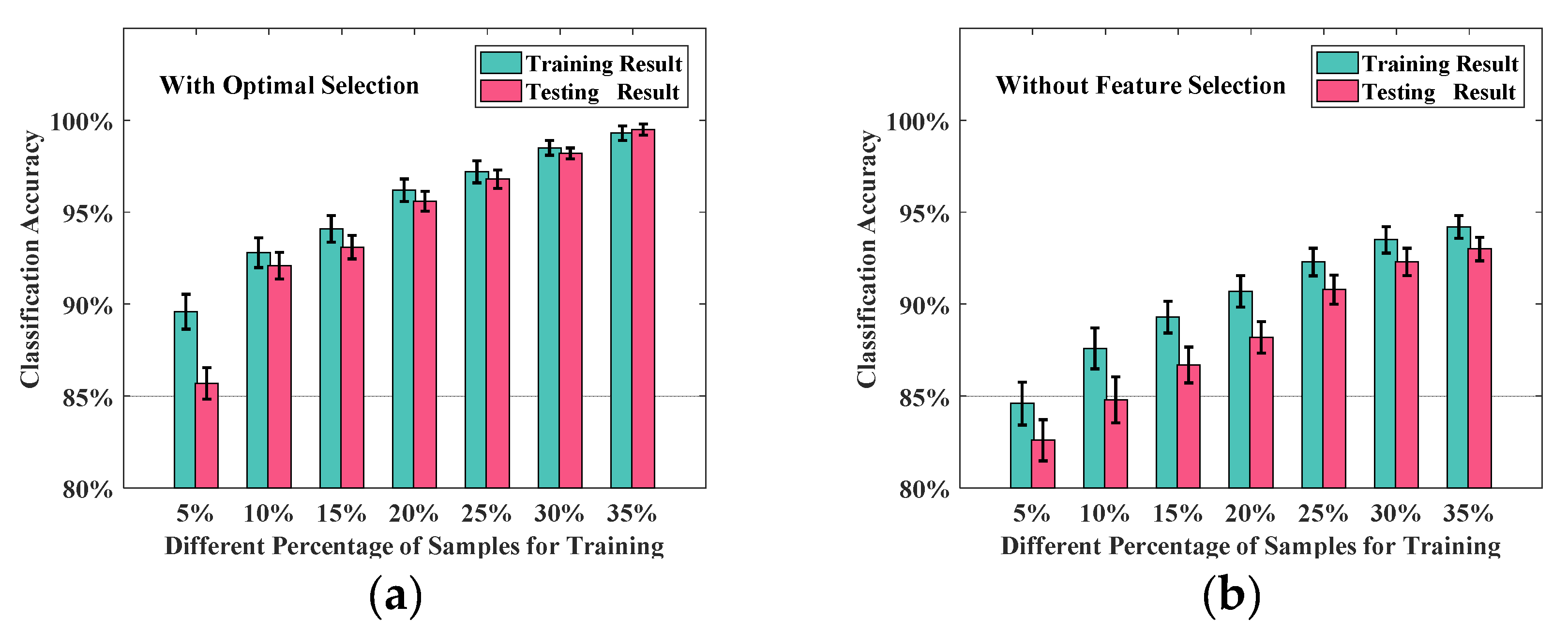
4.4. Performance Analysis

The performance of the proposed method can be depicted by the following values: precision for the correctly identified type of PQD, P_occur; recall for the correctly identified type of PQD, R_occur; precision for the incorrectly identified type of PQD, P_other; and, recall for the incorrectly identified type of PQD, R_other.

$$\begin{array}{l}{P}_{defect}=\frac{TP}{TP+FP}\\ R_{defect}=\frac{TP}{TP+FN}\\ P_{other}=\frac{TN}{TN+FN}\\ R_{other}=\frac{FP}{FP+TN}\\ A\mathrm{ccuracy}=\frac{TP+TN}{TP+FP+TN+FN}\times 100\%\end{array}$$

(14)

As shown in Equation (14), TP represents the number of true positive instances, which means that the estimated PQD type is correctly classified. FP represents the number of false positive instances, which means that another PQD is classified incorrectly as the estimated PQD type. FN represents the number of false negative instances, which means that the estimated PQD type is incorrectly classified as another PQD type. TN represents the number of true negative instances, which means that another PQD type is correctly identified as the corresponding PQD.

Table 3. Confusion matrix of PQD classification.

Assigned Class	True Class
	C1	C2	C3	C4	C5	C6	C7	C8	C9	C10	C11	C12	C13
C1	418	0	0	0	0	0	0	0	0	0	0	0	0
C2	0	394	0	4	0	0	0	0	0	0	0	0	0
C3	0	0	390	0	0	0	0	0	0	0	0	0	0
C4	0	5	0	411	0	0	0	0	0	0	0	0	0
C5	0	0	0	0	397	0	0	0	0	0	0	0	0
C6	0	0	0	0	0	427	0	0	0	0	0	0	0
C7	0	0	0	0	0	0	407	0	0	0	0	0	0
C8	0	0	0	0	0	0	0	396	0	0	0	0	0
C9	0	0	0	0	0	0	0	0	407	0	0	0	0
C10	0	0	0	0	0	0	0	0	0	406	0	0	0
C11	0	0	0	0	0	0	0	0	0	0	401	3	4
C12	0	0	0	0	0	0	0	0	0	0	3	413	0
C13	0	0	0	0	0	0	0	0	0	0	3	0	398

presents the confusion matrix of the PQD classification for the validation data sets. The classification results achieve high accuracy, as observed from the confusion matrix. However, there are still some mistakes due to the similar characteristics of some PQD types. For instance, two C4 (Interrupt Disturbances) samples are incorrectly assigned to C2 (Sag). Meanwhile, three C2 samples are also incorrectly assigned to C4, because the formula definitions of C2 and C4 are the same, and the only difference between these two classes is parameter α. As referred to above in Table 2, parameter α randomly varies over a range. To be specific, for C2 (sag), the range of parameter α is from 0.1 to 0.9. For C4 (interrupt) and the range of parameter α is from 0.9 to 1. When parameter α is selected to be near for both classes, the features that were extracted from the signal are also similar. In this circumstance, it would lead to an incorrect classification. The results for C11 (Sag with harmonics) and C13 (Interruption with harmonics) also verify this situation.

The receiver operating characteristic (ROC) curve is adopted to depict the tradeoff relationship between the true positive rate and the false positive rate to evaluate the performance of the proposed classifier, as shown in Figure 12. Ten OVR classifiers were constructed due to the ten PQD types since the “one-versus-rest” (OVR) structure was utilized for multiclass classification in this paper. Subsequently, ten ROC curves were drawn to represent the true positive rate versus the false positive rate at various threshold values of θ. To be specific, the threshold varied from 0 to 1 with a step of 0.02. By giving the threshold θ, the average values of the true positive rate and false positive rate were calculated. The areas of the four ROC curves from the C1 class to the C10 class were 0.979, 0.958, 0.949, 0.963, 0.957, 0.978, 0.947, 0.965, 0.986, and 0.987. For the PQD classification, a large false positive rate would cause false alarms, which would result in unexpected or even mistaken strategy responses for power grids. More seriously, a large false positive rate would lead to worse consequences in the distribution generation systems with high penetration. By contrast, a small true positive rate would degrade the usability of the PQD detecting system. Being observed from the ROC curves, the proposed method has enough flexibility to satisfy various requirements, either for the disturbance-detected sensitivity or specificity.

4.5. Accuracy Under a Real Noisy Environment

The signals in the real power systems are contaminated with the high probability of containing noise. Therefore, an artificial test signal is constructed with different intensities of white Gaussian noise (AWGN). The intensity of the white Gaussian noise is given as the signal to noise ratio (SNR), which is defined in Equation (10), where Ps and Pn are the power of the signal and noise, respectively.

Table 4. Performance of PQD classification accuracy under a noisy environment.

Assigned Class	Signal to Noise Ratio
	20 dB	30 dB	40 dB	50 dB
C1	100%	100%	100%	100%
C2	95.4%	98.2%	98.8%	99.2%
C3	99.2%	100%	100%	100%
C4	100%	100%	100%	100%
C5	94.2%	97.8%	97.8%	99.6%
C6	94.4%	98.0%	99.6%	100%
C7	97.6%	99.6%	99.6%	99.6%
C8	100%	100%	100%	100%
C9	100%	100%	100%	100%
C10	98.0%	98.4%	99.8%	100%
C11	95.4%	95.8%	97.2%	98.8%
C12	96.2%	96.6%	97.6%	98.4%
C13	95.6%	97.8%	98.6%	99.2%
Overall	97.38%	98.63%	99.15%	99.60%

shows the performance of the proposed classifier under different SNRs between 20 and 50 dB, which is conducted on the real microgrid platform. The robustness of the proposed algorithm is tested for 500 test samples for each PQD class in the presence of noise. The type of PQD events and the number of PQD events are selected in random series during the test stage. Overall, the classification accuracy decreases as the SNR level decreases. Nevertheless, the classification accuracy still reaches greater than 94%, even if the SNR drops to 20 dB. The results demonstrate that the SVM classifier of the proposed algorithm is less sensitive in a noisy environment. The reason that the classifier is insensitive to noise is attributed to the satisfactory performance of the algorithm. Each mode has a central frequency with a narrow bandwidth since VMD decomposes the signal into band-limited modes by updating with Wiener filtering. In this method, the disturbance signal is effectively separated from noise, which benefits the procedure of feature extraction for the SVM classifier.

5. Conclusions

This paper proposes a novel approach for PQD detection and classification. At the first stage, the proposed algorithm takes advantage of VMD to decompose the obtained signal into a series of intrinsic mode functions. Subsequently, the statistical features, such as RMS, standard deviation, and multiscale moments, are extracted from each IMF. Subsequently, a two-stage heuristic feature selection algorithm is introduced to rank the dominant features based on permutation entropy and the Fisher score. Finally, the reconstructed feature vectors are imported into a multiclass SVM classifier for training to identify the different types of PQD signals. The artificial dataset of the PQD signals is utilized for the model training and developing in order to improve the robust of the PQD classifier. Subsequently, the trained model is tested on the real experimental setup. Several analysis methods, such as confusion matrix and receiver operating characteristic (ROC) curve, are imported and analyzed the performance of the trained classifier model. Afterwards, the trained model is tested on the real microgrid platform to verify the effectiveness of the proposed algorithm.

The conclusions of this research are summarized, as follows. Signal preprocessing is obligatory at the first stage. The VMD process is beneficial for both signal de-noising and PQD detection. The permutation entropy analysis had the ability to identify useful IMFs that were obtained from VMD, which is vital in the feature selection process. By identifying the dominant features, the accuracy and the computational efficiency are both improved. Particularly, permutation entropy combined with the Fishe score showed better performance in ranking the relevant features. According to the real experimental data analysis, the proposed approach showed enough flexibility under different noisy environments, either for PQD detection sensitivity or specificity.

References

1. Mesbah, M.; Moses, P.S.; Islam, S.M.; Masoum, M.A.S. Digital implementation of a fault emulator for transient study of power transformers used in grid connection of wind farms. IEEE Trans. Sustain. Energy 2014, 5, 646–654. [Google Scholar] [CrossRef]
2. Fu, L.; Wei, Y.D.; Fang, S.; Tian, G.; Zhou, X.J. A wind energy generation replication method with wind shear and tower shadow effects. Adv. Mech. Eng. 2018, 10, 3. [Google Scholar] [CrossRef]
3. Teke, A.; Saribulut, L.; Tumay, M. A Novel Reference Signal Generation Method for Power-Quality Improvement of Unified Power-Quality Conditioner. IEEE Trans. Power Deliv. 2011, 26, 2205–2214. [Google Scholar] [CrossRef]
4. Ahila, R.; Sadasivam, V.; Manimala, K. An integrated PSO for parameter determination and feature selection of ELM and its application in classification of power system disturbances. Appl. Soft. Comput. 2015, 32, 23–37. [Google Scholar] [CrossRef]
5. Brenna, M.; Faranda, R.; Tironi, E. A New Proposal for Power Quality and Custom Power Improvement: OPEN UPQC. IEEE Trans. Power Deliv. 2009, 24, 2107–2116. [Google Scholar] [CrossRef]
6. Khokhar, S.; Zin, A.A.M.; Mokhtar, A.S.; Ismail, N.A.M. MATLAB/Simulink Based Modeling and Simulation of Power Quality Disturbances. In Proceedings of the IEEE Conference on Energy Conversion (CENCON), Johor Bahru, Malaysia, 13–14 October 2014; pp. 445–450. [Google Scholar]
7. Mahela, O.P.; Shaik, A.G.; Gupta, N. A critical review of detection and classification of power quality events. Renew. Sustain. Energy Rev. 2015, 41, 495–505. [Google Scholar] [CrossRef]
8. IEEE Recommended Practice for Monitoring Electric Power Quality; IEEE Standards Board, IEEE Std. 1159–1995; IEEE Inc.: New York, NY, USA, 1995; p. 6.
9. Standard Definitions for the Measurement of Electric Power Quantities Under Sinusoidal, Non-Sinusoidal, Balanced, or Unbalanced Conditions; Revision of IEEE Std. 1459–2000, IEEE Standard 1459–2010; IEEE Inc.: New York, NY, USA, 2010; p. 3.
10. José, C.A.; Salvador, O.; Nicolás, M.; Francisco, J.G.; Salvador, S. Measurement system for a power quality improvement structure based on IEEE Std. 1459. IEEE Trans. Instrum. Meas. 2013, 62, 3177–3188. [Google Scholar] [CrossRef]
11. Kanirajan, P.; Kumar, V.S. Power quality disturbance detection and classification using wavelet and RBFNN. Appl. Soft. Comput. 2015, 35, 470–481. [Google Scholar] [CrossRef]
12. He, S.F.; Li, K.C.; Zhang, M. A Real-Time Power Quality Disturbances Classification Using Hybrid Method Based on S-Transform and Dynamics. IEEE Trans. Instrum. Meas. 2013, 62, 2465–2475. [Google Scholar] [CrossRef]
13. Ray, P.K.; Mohanty, S.R.; Kishor, N.; Catalao, J.P.S. Optimal Feature and Decision Tree-Based Classification of Power Quality Disturbances in Distributed Generation Systems. IEEE Trans. Sustain. Energy 2014, 5, 200–208. [Google Scholar] [CrossRef]
14. Jurado, F.; Saenz, J.R. Comparison between discrete STFT and wavelets for the analysis of power quality events. Electr. Power Syst. Res. 2002, 62, 183–190. [Google Scholar] [CrossRef]
15. Eristi, H.; Ucar, A.; Demir, Y. Wavelet-based feature extraction and selection for classification of power system disturbances using support vector machines. Electr. Power Syst. Res. 2010, 80, 743–752. [Google Scholar] [CrossRef]
16. Biswal, B.; Dash, P.K.; Panigrahi, B.K. Non-stationary power signal processing for pattern recognition using HS-transform. Electr. Appl. Soft. Comput. 2009, 9, 107–117. [Google Scholar] [CrossRef]
17. Zhang, Y.; Ji, T.Y.; Li, M.S.; Wu, Q.H. Identification of Power Disturbances Using Generalized Morphological Open-Closing and Close-Opening Undecimated Wavelet. IEEE Trans. Ind. Electron. 2016, 63, 2330–2339. [Google Scholar] [CrossRef]
18. Camarena-Martinez, D.; Valtierra-Rodriguez, M.; Perez-Ramirez, C.A.; Amezquita-Sanchez, J.P.; Romero-Troncoso, R.D.; Garcia-Perez, A. Novel Downsampling Empirical Mode Decomposition Approach for Power Quality Analysis. IEEE Trans. Ind. Electron. 2016, 63, 2369–2378. [Google Scholar] [CrossRef]
19. Shukla, S.; Mishra, S.; Singh, B. Empirical-Mode Decomposition with Hilbert Transform for Power-Quality Assessment. IEEE Trans. Power Deliv. 2009, 24, 2159–2165. [Google Scholar] [CrossRef]
20. Lima, M.A.A.; Cerqueira, A.S.; Coury, D.V.; Duque, C.A. A novel method for power quality multiple disturbance decomposition based on Independent Component Analysis. Int. J. Electr. Power Energy Syst. 2012, 42, 593–604. [Google Scholar] [CrossRef]
21. Dragomiretskiy, K.; Zosso, D. Variational mode decomposition. IEEE Trans. Signal Process. 2014, 62, 531–544. [Google Scholar] [CrossRef]
22. Fu, L.; Wei, Y.D.; Fang, S.; Zhou, X.J.; Lou, J.Q. Condition Monitoring for Roller Bearings of Wind Turbines Based on Health Evaluation under Variable Operating States. Energies 2017, 10, 1564. [Google Scholar] [CrossRef]
23. Achlerkar, P.D.; Samantaray, S.R.; Manikandan, M.S. Variational Mode Decomposition and Decision Tree Based Detection and Classification of Power Quality Disturbances in Grid-Connected Distributed Generation System. IEEE Trans. Smart Grids 2018, 9, 3122–3132. [Google Scholar] [CrossRef]
24. Abdoos, A.A.; Mianaei, P.K.; Ghadikolaei, M.R. Combined VMD-SVM based feature selection method for classification of power quality events. Appl. Soft. Comput. 2016, 38, 637–646. [Google Scholar] [CrossRef]
25. Fu, L.; Zhu, T.T.; Zhu, K.; Yang, Y.L. Condition Monitoring for the Roller Bearings of Wind Turbines under Variable Working Conditions Based on the Fisher Score and Permutation Entropy. Energies 2019, 12, 3085. [Google Scholar] [CrossRef]
26. Wang, Y.X.; Liu, F.Y.; Jiang, Z.S.; He, S.L.; Mo, Q.Y. Complex variational mode decomposition for signal processing applications. Mech. Syst. Signal Proc. 2018, 86, 75–85. [Google Scholar] [CrossRef]
27. Zhu, T.; Qu, Z.; Xu, H.; Zhang, J.; Shao, Z.; Chen, Y.; Prabhakar, S.; Yang, J. RiskCog: Unobtrusive real-time user authentication on mobile devices in the wild. IEEE Trans. Mob. Comput. 2019. [Google Scholar] [CrossRef]
28. Tan, D.P.; Li, P.Y.; Ji, Y.X.; Wen, D.H.; Li, C. SA-ANN-based slag carry-over detection method and the embedded WME platform. IEEE Trans. Ind. Electron. 2013, 60, 4702–4713. [Google Scholar] [CrossRef]
29. Bhuiyan, S.M.A.; Khan, J.; Murphy, G. WPD for Detecting Disturbances in Presence of Noise in Smart Grid for PQ Monitoring. IEEE Trans. Ind. Appl. 2018, 54, 702–711. [Google Scholar] [CrossRef]
30. Zhang, X.Y.; Liang, Y.T.; Zhou, J.Z.; Zang, Y. A novel bearing fault diagnosis model integrated permutation entropy, ensemble empirical mode decomposition and optimized SVM. Measurement 2015, 69, 164–179. [Google Scholar] [CrossRef]
31. Tan, D.P.; Li, L.; Zhu, Y.L.; Zheng, S.; Ruan, H.J.; Jiang, X.Y. An embedded cloud database service method for distributed industry monitoring. IEEE Trans. Ind. Inf. 2018, 14, 2881–2893. [Google Scholar] [CrossRef]
Figure 1. Flow chart of the VMD algorithm.
Applsci 09 04901 g001
Figure 2. Main flow chart of the proposed method.
Applsci 09 04901 g002
Figure 3. The diagram of the “one-versus-rest” (OVR) multiclass strategy.
Applsci 09 04901 g003
Figure 4. Experimental setup for power quality disturbances.
Applsci 09 04901 g004
Figure 5. The architecture diagram of the experimental setup.
Applsci 09 04901 g005
Figure 6. Original signal of interruption with harmonics.
Applsci 09 04901 g006
Figure 7. Power quality disturbances (PQD) signal decomposition results by variational mode decomposition (VMD). (a) When K = 3 by VMD; (b) when K = 4 by VMD; (c) when K = 5 by VMD; and, (d) when K = 6 by VMD.
Applsci 09 04901 g007
Figure 8. PQD signal decomposition results by WPD. (a) When the decomposition level is 2 by WPD; and, (b) when the decomposition level is 3 by WPD.
Applsci 09 04901 g008
Figure 9. Correlation between features and classification accuracy.
Applsci 09 04901 g009
Figure 10. Identification accuracy results with different numbers of selected features. (a) Training result only by Fisher’s scoring method; and, (b) training result by Fisher’s score and the permutation entropy method.
Applsci 09 04901 g010
Figure 11. Accuracy comparison with different training percentages. (a) classification accuracy with feature heuristic selection; and, (b) classification accuracy without feature selection.
Applsci 09 04901 g011
Figure 12. Receiver operating characteristic curve for each PQD class.
Applsci 09 04901 g012