Hyperspectral Image Classification Based on Spectral and Spatial Information Using Multi-Scale ResNet

Featured Application

In this paper, a multi-scale ResNet is proposed for hyperspectral image classification, which can be applied in biohazard detection, agriculture, wasteland fire tracking, and environmental science.

Abstract

Hyperspectral imaging (HSI) contains abundant spectrums as well as spatial information, providing a great basis for classification in the field of remote sensing. In this paper, to make full use of HSI information, we combined spectral and spatial information into a two-dimension image in a particular order by extracting a data cube and unfolding it. Prior to the step of combining, principle component analysis (PCA) is utilized to decrease the dimensions of HSI so as to reduce computational cost. Moreover, the classification block used during the experiment is a convolutional neural network (CNN). Instead of using traditionally fixed-size kernels in CNN, we leverage a multi-scale kernel in the first convolutional layer so that it can scale to the receptive field. To attain higher classification accuracy with deeper layers, residual blocks are also applied to the network. Extensive experiments on the datasets from Pavia University and Salinas demonstrate that the proposed method significantly improves the accuracy in HSI classification.

1. Introduction

Hyperspectral image classification plays one of the most fundamental and important roles in remote sensing. It uses computers and other tools to quickly classify each pixel in an image into different classes, so as to achieve the ground observation and object recognition. Unlike a two-dimensional color image, Hyperspectral imaging (HSI) is a three-dimensional data cube with hundreds of narrow and continuous spectral bands, providing great potential for the subsequent information extraction [1,2]. In HSI, each spectral band is an ordinary two-dimensional image, and each pixel almost corresponds to a continuous spectral curve. The spectral curves of each land-cover class vary due to their different reflectance to light of various frequencies, which means that HSI classification assigns a specific set of categories to each pixel based on its spectral information [3].

However, the high dimension of HSI easily leads to the problem of the curse of dimensionality, which increases the complexity of calculation and decreases the accuracy of classification. In addition, HSI data usually contains a small number of labelled samples and the sample distribution is not balanced, easily resulting in an overfitting problem for the class with fewer samples. Due to the inherent characteristics of hyperspectral images, HSI classification is facing great difficulties. Various methods have been proposed to classify HSI, such as the K-nearest neighbor (KNN) algorithm [4], partial least squares-discriminant analysis (PLS-DA) [5], discriminant analysis (DA) or soft independent modeling of class analogy (SIMCA) [6], random forest (RF) [7], support vector machine (SVM) [8,9], and extreme learning machine (ELM) [10]. However, most of these traditional algorithms encounter the “curse of dimensionality”. Various methods have been developed to deal with HSI classification problems [11,12,13,14,15,16,17,18,19,20,21,22,23,24]. In recent years, many research results in image classification have been obtained with deep learning methods, especially convolutional neural networks. These exciting results demonstrate its powerful feature extraction capabilities in computer vision competition, which brings great opportunities for the development of HSI classification [25]. In 2015, Hu et al. [26] trained a one-dimensional CNN to directly classify a pixel of a hyperspectral image and obtained 92.56% accuracy on the dataset from Pavia University. The architecture of the network was very simple, with only five layers. In 2016, a contextual deep CNN was used to classify HSI by Hyungtae et al. [27], which obtained 94.06% accuracy in the same dataset. In 2017, Kussul et al. used one-dimensional and two-dimensional CNNs to classify crops, and they concluded that the effect of two-dimensional CNN was better than one-dimensional CNN [28]. Recently, classification methods based on spectral–spatial methods have made great progress in HSI classification, showing that they have higher classification accuracy, such as the methods proposed in the papers [29,30,31,32]. Although these methods above, based on spectral information classification, can classify HSI effectively, most of them did not consider either dimension reduction of data or spatial information in HSI, likely leading to many noisy points in the classification maps and heavy computation.

In a similar way, in this paper, we introduce a novel classification algorithm based on two-dimensional CNN that combines spectral and spatial features. The main contributions of this paper are listed below.

• To reduce the correlation between HSI spectral bands and the amount of computation, the principle component analysis (PCA) method is used to preprocess the HSI data.
• Spatial and spectral features are combined ahead of feeding into the classification model.
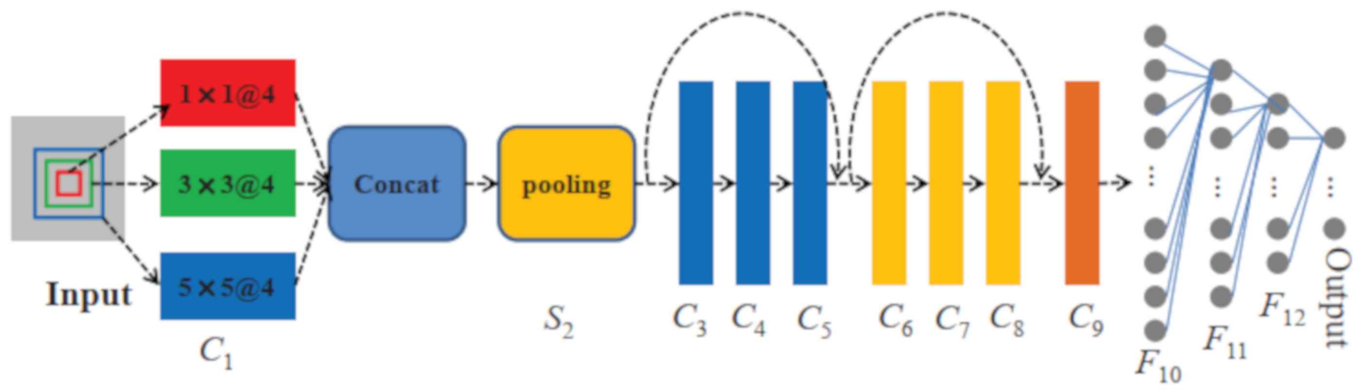
• To fully extract the most important information and reduce the risk of overfitting, multi-scale kernels are applied to the first convolutional layer.
• To protect the integrity of information and deepen the network, residual blocks are added to the network.

2. Related Works

2.1. CNN for Classification

The first convolutional neural network (CNN) so called LeNet-5 [33] consists of only five layers. With the recent advent of large scale image databases, the network becomes relatively deeper and wider. Hence, The feature extraction ability of networks has been enhanced dramatically from the original LeNet [33], to VGG-16 [34], to GoogleNet [35], to residual networks (ResNets), which have surpassed 100 layers [36], and to wide-residual networks [37]. The ResNets introduce the skip-connection layer, which creates shorter paths between earlier and later layers, to avoid the problems of gradient vanishing and feature propagation emergence caused by a very deep network.

2.2. Hyperspectral Image Classification

Most existing methods deal with the classification of hyperspectral images according to the conventional paradigm of pattern recognition, which is built on complex hand crafted features and shallow trainable classifiers, such as support vector machines (SVM) [38] and neural networks (NN) [39]. However, due to the high diversity of depicted materials, they are highly reliant on domain knowledge to determine which features are important for the classification task. A large number of deep learning models, capable of automatically discovering and learning semantic features, have been developed to tackle HSI classification problems [24,40,41,42,43]. Chen et al. [40] introduced the concept of deep learning into hyperspectral data classification for the first time. Chen et al. [41] employed several convolutional and pooling layers to extract deep features from HSIs, which are nonlinear, discriminant, and invariant. Ran et al. [42] proposed a spatial pixel pair feature that better exploits both the spatial/contextual information and spectral information for HSI classification. In [24], the image was firstly segmented into different homogeneous parts, called superpixels. Then a superpixel-based multitask learning framework was proposed for hyperspectral image classification. Mou et al. [43] proposed a novel recurrent neural network(RNN) model that can effectively analyze hyperspectral pixels as sequential data and then determine information categories via network reasoning. These approaches normally require large scale datasets whose size should be proportional to the number of parameters used by the network to avoid overfitting.

Unlike these deep learning-based approaches, we first reduce the computation by decreasing the dimensions of HSI with PCA. Then, a multi-scale network is proposed to expand the receptive filed and automatically capture spectral and spatial feature. Finally, we fuse the features and feed into the CNN model.

3. The Proposed Method

3.1. Data Preprocessing

As mentioned above, HSI has high dimensions and the data among adjacent spectral bands have strong correlations. If the raw data are trained directly, it may cause unnecessary calculation and even reduce the accuracy and speed of classification. Therefore, the PCA method [44,45] is used to reduce the dimensions of HSI. During the experiment processing on extensively-used datasets of HSI, the first 25 principle components are selected, which remains at least 99% of the initial information. In HSI, the spectral information is connected with the reflectance properties of each pixel on each spectral band. Differently, the spatial information is derived by considering its neighborhood pixels [29]. Therefore, in this paper, spectral and spatial information are combined as samples. For the sake of brevity, we call the samples combined with spatial and spectral information, SS Images. The sample generation process is shown in Figure 1.

The detailed sampling procedure is described as the following.

• After PCA is conducted, we assume that a labelled pixel $p_{i,j}$ at location of $(i,j)$ is selected as a sample, and labeled as the class of $l_{i,j}$.
• Then, we center on pixel $p_{i,j}$, increase the rows and columns from $(i-2,j-2)$ to $(i+2,j+2)$ respectively, and capture an area of $5\times 5$ to form a three-dimensional cube of $5\times 5\times c_r$.
• Finally, the three-dimensional cube is unfolded by extracting the spectral band values of each pixel to form a row vector from left to right and from top to bottom, thus a $25\times c_r$ image is formed as shown in Figure 2, which combine spectral and spatial information as an input, denoted as $x_{i,j}$. A sample of $d_{i,j}$, an SS Image, is formed as $d_{i,j}=(x_{i,j},l_{i,j})$.
• Repeat steps (1–3), and we can form the dataset $D=\{d_{i,j},i=1,2,...,w,j=1,2,...,h\}$.

3.2. Network Architecture

This part describes in detail the architecture of the network, the model used in the experiments. Except for the input layer, the model is comprised of 12 layers, all of which contain trainable parameters, as shown in Figure 3. All convolution layers use the same convolution operation, so that more information of the image can be retained. For convenience, let $C_x$, $S_x$, and $F_x$ denote convolutional layers, sub-sampling layers, and fully-connected layers, respectively, where x is the index of each layer.

Layer $C_1$ is a multi-scale kernel convolutional layer which can expand to the receptive filed. The convolution operation is carried out with convolution kernel of the size of $1\times 1$, $3\times 3$, and $5\times 5$. Each convolution module has 4 kernels and the output feature maps are concatenated after they pass through a rectified linear unit (ReLU) function.

Layer $S_2$ is a max pooling layer with 12 feature maps. Since the $2\times 2$ receptive fields do not overlap, the number of rows and columns of the feature map in $S_2$ is half of the feature map in $C_1$.

Layers $C_3$–$C_9$ are convolutional layers with $3\times 3$ kernels. Two residual blocks are added to the network which can attain higher classification accuracy with deeper layers. The last convolutional layer $C_9$ outputs 32 feature maps.

Layer $F_{10}$ and layer $F_{11}$ are fully-connected layers with 120 and 84 units, respectively. To decrease the risk of overfitting, the dropout method is conducted.

The last layer $F_{12}$ is also a fully connected layer, which is also the output layer of the model. The number of neuron units are related to the number of classes. Since it implements a multi-classification task, Softmax regression is used in this layer.

3.3. Loss Function

Considering the huge distinction in the number of each category, the dice coefficient was used as the loss function. The dice coefficient is used to compare the similarity of two batches of data, usually for binary image segmentation, i.e., when the label is binary. The dice coefficient results in a value of 0 to 1, where 1 indicates an exact match.

$$D=1-\frac{2|X\cap Y|}{\left|X\right|+\left|Y\right|}.$$

(1)

The network predictions $p_i$, which contain k dimension, are processed through a soft-max layer which outputs the probability of each pixel to belong to different classes. Parameter k is the number of classes. According to the dice coefficient, we propose an objective function. The loss function is defined as the following:

$$L=1-\frac{2{\sum }_i^N{p}_i{g}_i}{{\sum }_i^N{p_i}^2+{\sum }_i^N{g_i}^2}$$

(2)

where $p_i$ is the output score and $g_i$ is the ground true label score. N stands for the number of pixels.

4. Experiment Results and Analysis

We evaluate the performance of the proposed method on two datasets from Pavia University and Salinas. The Pavia University dataset contains 103 bands, which covers the wavelength from 430 nm to 860 nm. It has $610\times 340$ pixels and nine classes to be classified. The Salinas dataset contains 204 bands, which covers the wavelength from 400 to 2500 nm with $512\times 217$ pixels and has 16 classes. Four commonly used performance metrics are utilized to evaluate the model: overall accuracy (OA), average accuracy (AA), kappa coefficient, and testing time. In the experiment, we randomly selected 200 samples per class as training sets (as shown in

Table 1. The number of training samples of the Pavia University dataset.

No.	Classes	Total Samples	Training Samples
1	Asphalt	6631	200
2	Meadows	18,649	200
3	Gravel	2099	200
4	Trees	3064	200
5	Painted metal sheets	1345	200
6	Bare Soil	5029	200
7	Bitumen	1330	200
8	Self-blocking bricks	3682	200
9	Shadows	947	200
Total		42776	1800

and

Table 2. The number of training samples of the Salinas dataset.

No.	Classes	Total Samples	Train Samples
1	Brocoli green weeds 1	2009	200
2	Brocoli green weeds 2	3726	200
3	Fallow	1976	200
4	Fallow rough plow	1394	200
5	Fallow smooth	2678	200
6	Stubble	3959	200
7	Celery	3579	200
8	Grapes untrained	11,271	200
9	Soil vinyard develop	6203	200
10	Corn senesced green weeds	3278	200
11	Lettuce romaine 4wk	1068	200
12	Lettuce romaine 5wk	1927	200
13	Lettuce romaine 6wk	916	200
14	Lettuce romaine 7wk	1070	200
15	Vinyard untrained	7268	200
16	Vinyard vertical trellis	1807	200
Total		54,129	3200

), and the rest of the samples for testing sets. All the experiments were conducted using Python 3.6 on a computer with an 11G GPU.

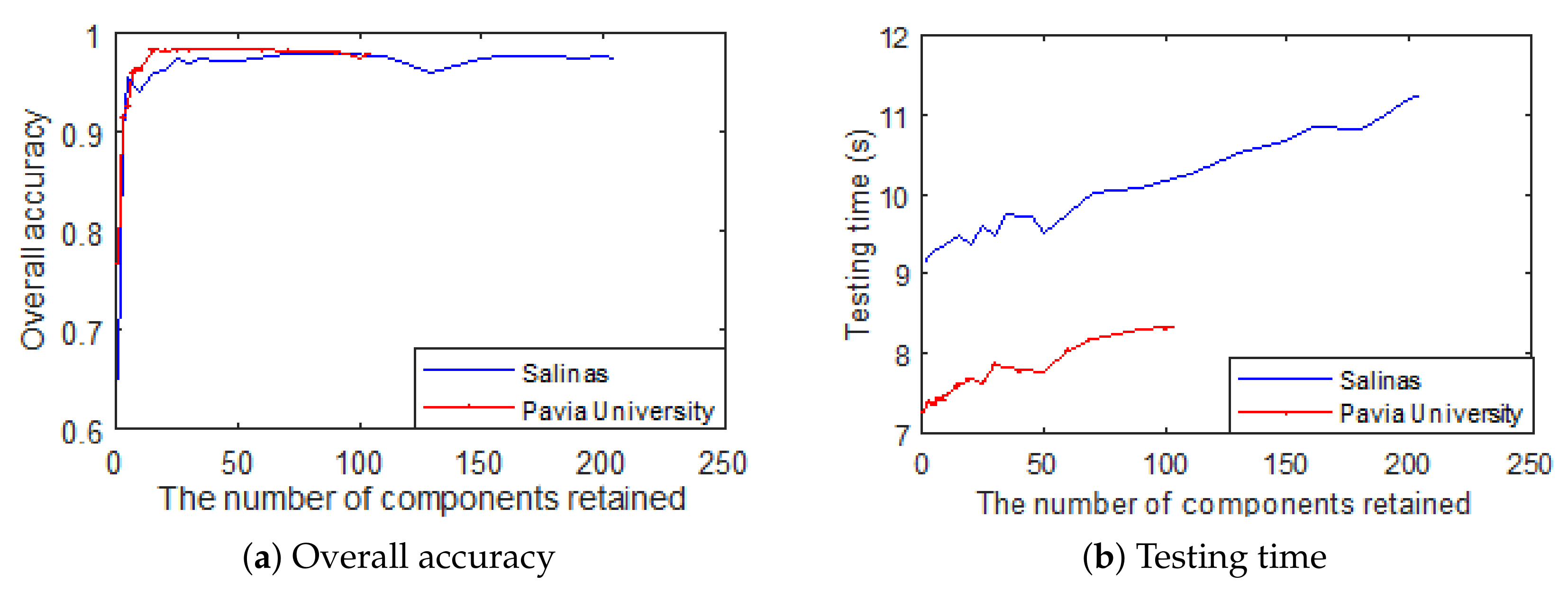
4.1. How Many Components Should Be Remained?

To test how many principal components should remain, we tested on the two datasets mentioned above. For the Pavia University dataset, the number of principal component components retained changes from 1 to 103, and for the Salinas data set, the number of principal component components retained changes from 1 to 204. The corresponding run time and overall accuracy are shown in Figure 4.

As can be seen from Figure 4, in the Salinas data set, when the number of components is less than 25, the more principal components that are retained, the higher the overall accuracy is that can be obtained. While in the data set of Pavia University, when the number of components is less than 15, the more principal component components that are retained, the higher the overall accuracy. However, from then on, the accuracy did not improve with an increase in the number of components. This is because these components have retained the information more than 99%. However, as the retained components increase, the testing time increases linearly. To balance time and efficiency, we set the number of components to 25 for the rest of experiments. Of course, the number can also be calculated automatically, for example, the number of reserved components can be determined automatically by requiring more than 99% of the information to be retained.

4.2. The Effect of the Cube Size

To demonstrate the effect of the extracted cube size in terms of overall accuracy of spectral–spatial method based on PCA, during the experiment, $3\times 3\times 9$, $4\times 4\times 16$, and $5\times 5\times 25$ cube data are extracted respectively and in each class, we selected 200 of samples randomly as training sets. The OA plot of the two datasets over the entire sample is shown in Figure 5. From Figure 5, we learn that the overall accuracy increases in both datasets with the increased cube size. This is because more contextual information, including spatial and spectral information, can be acquired with the increased cube size. In the experiment, both datasets achieve above 96% classification accuracy when the cube size is $5\times 5\times 25$.

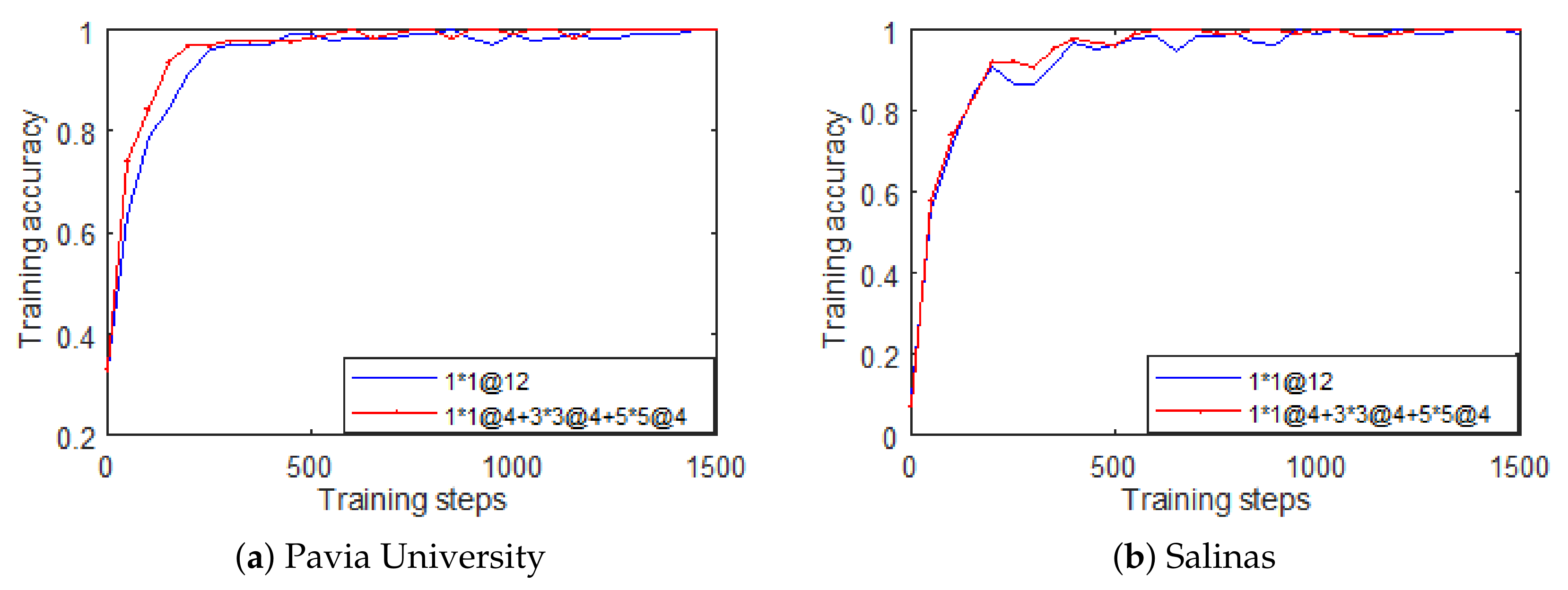
4.3. How the Multi-Scale Affects the Classification

In order to test the influence of the multi-scale convolutional kernel, we conducted six sets of experiments. In these experiments, the cube size is set to $5\times 5\times 25$. The first three experiments are convolution kernels with only one scale, whose convolution kernels are 1*1@12, 3*3@12 and 5*5@1 respectively. The fourth and fifth are the combination of two scale convolutional kernels, which are respectively the concatenation of 1*1@6+3*3@6, and the concatenation of 3*3@6+5*5@6. The sixth experiment is a concatenation of three scale convolution kernels: 1*1@4+3*3@4+5*5@4, as shown in Figure 6. Detailed results of the experiments are shown in

Table 3. The accuracy affected by multi-scale kernels. Overall accuracy (OA), average accuracy (AA). The best results are highlighted in bold.

Datasets	Kernels	Training Time	Testing Time	OA	AA	Kappa
Pavia University	1*1@12	26.40	7.32	0.963604	0.956682	0.951763
	3*3@12	26.15	7.23	0.978551	0.97294	0.971562
	5*5@12	26.23	7.30	0.97834	0.966848	0.971356
	1*1@6+3*3@6	26.93	7.45	0.978551	0.97294	0.971562
	3*3@6+5*5@6	26.84	7.48	0.978995	0.968616	0.972227
	1*1@4+3*3@4+5*5@4	27.57	7.49	0.986153	0.983208	0.981648
Salinas	1*1@12	25.96	8.95	0.957255	0.982387	0.952307
	3*3@12	26.13	9.04	0.965719	0.982829	0.961777
	5*5@12	26.12	9.27	0.964592	0.983698	0.96056
	1*1@6+3*3@6	26.63	9.17	0.971393	0.986391	0.968131
	3*3@6+5*5@6	27.04	9.28	0.974165	0.98662	0.971259
	1*1@4+3*3@4+5*5@4	27.61	9.53	0.975608	0.986853	0.972731

.

As can be seen from Table 3, the best results highlighted in bold were obtained by the last group while combining three scale convolution kernels. This is because multiple scales can get both local and global information.

We also plotted convergence curves with different kernels, as shown in Figure 7. The multi-scale kernel model can make the training convergence more stable in both the datasets.

4.4. The Performance of Classification on the Salinas and Pavia University Datasets

In this part, the three methods based on spectral, spectral + PCA, and spectral–spatial + PCA are compared. Among them, the method based on spectral does not carry out PCA preprocessing on the original hyperspectral image, but only normalization. Therefore, each pixel contains all the spectral information of the original image, and such a pixel containing all the original spectral information is taken as a sample. For the method based on spectral + PCA, PCA preprocessing is carried out after normalization, and then the first $c_r$ principal components are selected to reconstruct the image. When extracting the pixel, it does not consider the information of the neighborhood pixel, so each pixel only contains $c_r$ components of the pixel. In this experiment, $c_r$ is set to 25. Spectral–spatial + PCA is the method proposed in this paper.

The label maps of ground truth were shown in Figure 8a and Figure 9a and the classification maps were shown in Figure 8b–d and Figure 9b–d. It has to be mentioned that the black background pixels were not considered for our classification purpose. The classification results including OA, AA, Kappa, and time were displayed in

Table 4. Classification results of the Salinas dataset, including classification accuracies for every class, AA, OA, Kappa, and Time obtained by methods based on spectral, spectral + PCA and spectral–spatial + PCA. The best results are highlighted in bold.

Class	Spectral	Spectral + PCA	Spectral-Spatial + PCA
1	96.17	99.75	100.00
2	99.81	99.87	100.00
3	99.75	96.96	100.00
4	99.21	99.21	99.93
5	98.36	98.32	98.58
6	99.77	99.70	100.00
7	99.64	99.61	99.80
8	70.00	87.19	91.40
9	99.03	99.15	99.97
10	93.90	92.01	97.28
11	95.97	98.97	99.81
12	99.74	96.16	99.95
13	98.47	99.56	99.67
14	98.97	96.92	98.97
15	70.50	57,31	88.80
16	99.11	99.28	99.78
OA	88.84	90.48	96.41
AA	93.73	91.15	98.09
Kappa	87.61	89.38	96.01
Time (s)	2.3799	1.3771	5.0755

and

Table 5. Classification results of the Pavia University dataset, including classification accuracies for every class, AA, OA, Kappa, and Time obtained by methods based on spectral, spectral + PCA and spectral–spatial + PCA. The best results are highlighted in bold.

Class	Spectral	Spectral + PCA	Spectral-Spatial + PCA
1	83.74	81.81	97.45
2	85.81	83.67	98.47
3	80.32	77.23	97.33
4	95.43	93.37	98.43
5	99.78	99.48	100.00
6	84.67	87.55	98.91
7	94.43	90.90	99.47
8	82.16	85.17	92.42
9	100.00	99.89	99.89
OA	86.48	85.43	97.89
AA	84.19	83.58	95.57
Kappa	82.46	81.18	97.22
Time (s)	1.3992	1.0734	4.2585

, and the best results for each category are highlighted in bold.

Space spectral combination method based on PCA: This method is proposed in this paper. Firstly, PCA dimension reduction is carried out on the original hyperspectral image, and then the information of the target pixel and all pixels in its neighborhood are extracted as sample data for training and classification.

Table 4 and Table 5 show that the proposed method almost obtains optimal performance across all categories, and it also displays the best classification performance compared with the other two methods in terms of OA, AA, and Kappa. The proposed method is about 6% to 12% higher than the other two methods in both datasets in terms of OA, showing a great improvement in HSI classification. Considering AA, the method proposed is about 4.3% to 12%, higher than the other two methods in both datasets. We can see classification accuracy from the kappa coefficient. The proposed method outperforms the other two methods. Moreover, the proposed method has 100% classification accuracy in class 1, 2, 3, and 6 in the Salinas dataset and in class 5 in the Pavia University dataset. Visually, as shown in Figure 8 and Figure 9, the noisy points are greatly decreased in spectral–spatial based on PCA method. The reason why the proposed method can make such a great improvement is that it can compensate the insufficient of spectral information only by utilizing the spatial dependence of pixels.

4.5. The Influence between the Number of Training Samples and the Classification

During the experiment, we changed the number of training samples to study the effects on the classification performance for various methods. Here, we set the parameters as same as used in Section 4.4. In each experiment, 50, 100, 150, and 200 samples are chosen randomly in each class as training sets, and the rest were set to be testing sets. The overall accuracy plots under different conditions are shown in Figure 10. As shown in Figure 10, in most cases, when the percentage of training samples increases, the overall accuracy also increases. Furthermore, the proposed method achieves about 93% classification accuracy in both datasets by using only 50 of samples in each class, which is higher than the other two methods when using 200 samples. Therefore, it can be said that the spectral–spatial method based on PCA uses less samples to obtain higher classification accuracy.

4.6. Comparison of other Proposed Methods

To verify the feasibility of the proposed method, we compare some other CNN-based methods proposed in recent years on the Salinas and Pavia University datasets, including the methods CNN in [26], CNN-PPF in [46] and CD-CNN in [47]. The architecture of the classifier, proposed by Hu et al., comprises an input layer, the convolutional layer, the max poolinglayer, the fully-connected layer, and the output layer with weights [26]. In paper of Wei et al., a pixel-pair method was proposed to markedly increase such a number. This will enable the advantages provided by CNN to be used as much as possible. For testing pixels, the trained CNN classifies the pairs of pixels created by combining the central pixel with each surrounding pixel, and then determines the final label through voting strategy [46]. In the paper by Lee et al. [47], a deep CNN, which was deeper and wider than any other deep network for HSI classification was described. Different from methods in CNN-based hyperspectral image classification, the proposed network—a contextual deep CNN—can best explore local contextual interactions, by jointly utilizing local spatial-spectral relationships of neighboring individual pixel vectors. By using a multi-scale convolution filter bank as the initial component of the proposed CNN pipeline, the joint development of spatial-temporal spectral information can be achieved. After that, the original spatial and spectral feature maps obtained from the multi-scale filter bank are combined together to form a joint spatial–spectral feature map that represents abundant spectral and spatial properties of the hyperspectral image. The joint feature map is then fed through a fully convolutional network that eventually predicts the corresponding label of each pixel vector.

In this experiment, 50, 100, 150, and 200 training samples for each class are set respectively. The overall accuracy is shown in

Table 6. Overall accuracy (%) versus different numbers of training samples per class for different methods. The best results are highlighted in bold.

Datasets	Methods	Numbers of Training Samples
		50	100	150	200
Salinas	CNN [26]	89.20	89.58	89.60	89.72
	CNN-PPF [46]	92.15	93.88	93.84	94.80
	CD-CNN [47]	82.74	98.58	-	95.42
	Proposed method	92.18	93.77	95.02	96.41
Pavia University	CNN [26]	86.39	88.53	90.89	92.27
	CNN-PPF [46]	88.14	93.35	94.97	96.48
	CD-CNN [47]	92.19	93.35	-	96.73
	Proposed method	94.34	96.25	97.64	97.89

. As it can be seen in the Table, when the number of training samples increases, the overall accuracy also increases. In the case of the same number of training samples, it is clear that the proposed method almost always outperforms other three methods.

We can see from the overall accuracy of the Salinas dataset, with 50 training samples in each category, the overall accuracy of the proposed method is 92.18%. The overall accuracy resulting from the method proposed is 9.44%, higher than the lowest one. With 100 training samples in each category, the overall accuracy of the proposed method is not the maximum. With 150 training samples in each category, the overall accuracy of the proposed method is 95.02%. The overall accuracy resulting from the method proposed is 5.42%, higher than the lowest one. With 200 training samples in each category, the overall accuracy of the proposed method is 96.41%. The overall accuracy resulting from the method proposed is 6.69%, higher than the lowest one.

We can see from the overall accuracy of the Pavia University dataset with 50 training samples in each category, the overall accuracy of the proposed method is 94.34%. The overall accuracy resulting from the method proposed is 7.95%, higher than the lowest one. With 100 training samples in each category, the overall accuracy of the proposed method is 96.25%. The overall accuracy resulting from the method proposed is 7.72%, higher than the lowest one. With 150 training samples in each category, the overall accuracy of the proposed method is 97.64%. The overall accuracy resulting from the method proposed is 6.75%, higher than the lowest one. With 200 training samples in each category, the overall accuracy of the proposed method is 97.89%. The overall accuracy resulting from the method proposed is 5.62%, higher than the lowest one.

The proposed method shows higher classification accuracy on Pavia University dataset as well as Salinas datasets.

5. Conclusions

In this paper, we proposed a novel multi-scale kernel CNN with residual blocks based on PCA using spectral–spatial information for hyperspectral image classification. To reduce redundant spectral information, PCA is used in data preprocessing. Moreover, to improve the classification performance we combined spectral–spatial information by extracting a data cube and unfolding it into a two-dimensional. The classification block used in this paper is a multi-scale kernel CNN which can effectively extract the most important information from the HSI pixels. In particular, using multi-scale kernels can expand the receptive field and thus reduce the risk of overfitting. To make the network go deeper, two residual blocks were applied to the network. Experimental results reveal that the proposed method outperforms the method using spectral information only, and other methods proposed based on CNN in recent years, in terms of overall accuracy assessment.

References

1. Bioucas-Dias, J.; Plaza, A.; Camps-Valls, G.; Scheunders, P.; Nasrabadi, N.; Chanussot, J. Hyperspectral Remote Sensing Data Analysis and Future Challenges. IEEE Geosci. Remote Sens. Mag. 2013, 1, 6–36. [Google Scholar] [CrossRef]
2. He, L.; Li, J.; Liu, C.; Li, S. Recent Advances on Spectral-Spatial Hyperspectral Image Classification: An Overview and New Guidelines. IEEE Trans. Geosci. Remote Sens. 2018, 56, 1579–1597. [Google Scholar] [CrossRef]
3. Camps-Valls, G.; Tuia, D.; Bruzzone, L.; Benediktsson, J.A. Advances in Hyperspectral Image Classification: Earth Monitoring with Statistical Learning Methods. IEEE Signal Process. Mag. 2014, 31, 45–54. [Google Scholar] [CrossRef]
4. Blanzieri, E.; Melgani, F. Nearest Neighbor Classification of Remote Sensing Images with the Maximal Margin Principle. IEEE Trans. Geosci. Remote Sens. 2008, 46, 1804–1811. [Google Scholar] [CrossRef]
5. Yang, X.; Hong, H.; You, Z.; Cheng, F. Spectral and Image Integrated Analysis of Hyperspectral Data for Waxy Corn Seed Variety Classification. Sensors 2015, 15, 15578–15594. [Google Scholar] [CrossRef]
6. Rutlidge, H.T.; Reedy, B.J. Classification of heterogeneous solids using infrared hyperspectral imaging. Appl. Spectrosc. 2009, 63, 172. [Google Scholar] [CrossRef]
7. Ham, J.; Chen, Y.; Crawford, M.M.; Ghosh, J. Investigation of the random forest framework for classification of hyperspectral data. IEEE Trans. Geosci. Remote Sens. 2005, 43, 492–501. [Google Scholar] [CrossRef]
8. Melgani, F.; Bruzzone, L. Support vector machines for classification of hyperspectral remote-sensing images. In Proceedings of the IEEE International Geoscience and Remote Sensing Symposium, Toronto, ON, Canada, 24–28 June 2002; Volume 1, pp. 506–508. [Google Scholar] [CrossRef]
9. Archibald, R.; Fann, G. Feature Selection and Classification of Hyperspectral Images with Support Vector Machines. IEEE Geosci. Remote Sens. Lett. 2007, 4, 674–677. [Google Scholar] [CrossRef]
10. Wei, L.; Chen, C.; Su, H.; Qian, D. Local Binary Patterns and Extreme Learning Machine for Hyperspectral Imagery Classification. IEEE Trans. Geosci. Remote Sens. 2015, 53, 3681–3693. [Google Scholar]
11. Gurram, P.; Kwon, H. Sparse Kernel-Based Ensemble Learning with Fully Optimized Kernel Parameters for Hyperspectral Classification Problems. IEEE Trans. Geosci. Remote Sens. 2013, 51, 787–802. [Google Scholar] [CrossRef]
12. Gu, Y.; Liu, T.; Jia, X.; Benediktsson, J.A.; Chanussot, J. Nonlinear Multiple Kernel Learning with Multiple-Structure-Element Extended Morphological Profiles for Hyperspectral Image Classification. IEEE Trans. Geosci. Remote Sens. 2016, 54, 3235–3247. [Google Scholar] [CrossRef]
13. Morsier, F.D.; Borgeaud, M.; Gass, V.; Thiran, J.P.; Tuia, D. Kernel Low-Rank and Sparse Graph for Unsupervised and Semi-Supervised Classification of Hyperspectral Images. IEEE Trans. Geosci. Remote Sens. 2016, 54, 3410–3420. [Google Scholar] [CrossRef]
14. Liu, J.; Wu, Z.; Li, J.; Plaza, A.; Yuan, Y. Probabilistic-Kernel Collaborative Representation for Spatial-Spectral Hyperspectral Image Classification. IEEE Trans. Geosci. Remote Sens. 2016, 54, 2371–2384. [Google Scholar] [CrossRef]
15. Wang, Q.; Gu, Y.; Tuia, D. Discriminative Multiple Kernel Learning for Hyperspectral Image Classification. IEEE Trans. Geosci. Remote Sens. 2016, 54, 3912–3927. [Google Scholar] [CrossRef]
16. Guo, B.; Gunn, S.R.; Damper, R.; Nelson, J. Customizing kernel functions for SVM-based hyperspectral image classification. IEEE Trans. Image Process. 2008, 17, 622–629. [Google Scholar] [CrossRef]
17. Yang, L.; Min, W.; Yang, S.; Rui, Z.; Zhang, P. Sparse Spatio-Spectral LapSVM With Semisupervised Kernel Propagation for Hyperspectral Image Classification. IEEE J. Sel. Top. Appl. Earth Obs. Remote Sens. 2017, 10, 2046–2054. [Google Scholar] [CrossRef]
18. Roscher, R.; Waske, B. Shapelet-Based Sparse Representation for Landcover Classification of Hyperspectral Images. IEEE Trans. Geosci. Remote Sens. 2016, 54, 1623–1634. [Google Scholar] [CrossRef]
19. Zehtabian, A.; Ghassemian, H. Automatic Object-Based Hyperspectral Image Classification Using Complex Diffusions and a New Distance Metric. IEEE Trans. Geosci. Remote Sens. 2016, 54, 4106–4114. [Google Scholar] [CrossRef]
20. Jia, S.; Jie, H.; Yao, X.; Shen, L.; Li, Q. Gabor Cube Selection Based Multitask Joint Sparse Representation for Hyperspectral Image Classification. IEEE Trans. Geosci. Remote Sens. 2016, 54, 3174–3187. [Google Scholar] [CrossRef]
21. Xia, J.; Chanussot, J.; Du, P.; He, X. Rotation-Based Support Vector Machine Ensemble in Classification of Hyperspectral Data With Limited Training Samples. IEEE Trans. Geosci. Remote Sens. 2016, 54, 1519–1531. [Google Scholar] [CrossRef]
22. Zhong, Z.; Fan, B.; Ding, K.; Li, H.; Xiang, S.; Pan, C. Efficient Multiple Feature Fusion With Hashing for Hyperspectral Imagery Classification: A Comparative Study. IEEE Trans. Geosci. Remote Sens. 2016, 54, 4461–4478. [Google Scholar] [CrossRef]
23. Xia, J.; Bombrun, L.; Adali, T.; Berthoumieu, Y.; Germain, C. Spectral-Spatial Classification of Hyperspectral Images Using ICA and Edge-Preserving Filter via an Ensemble Strategy. IEEE Trans. Geosci. Remote Sens. 2016, 54, 4971–4982. [Google Scholar] [CrossRef]
24. Jia, S.; Deng, B.; Zhu, J.; Jia, X.; Li, Q. Superpixel-Based Multitask Learning Framework for Hyperspectral Image Classification. IEEE Trans. Geosci. Remote Sens. 2017, 55, 2575–2588. [Google Scholar] [CrossRef]
25. Lecun, Y.; Bengio, Y.; Hinton, G. Deep learning. Nature 2015, 521, 436. [Google Scholar] [CrossRef]
26. Hu, W.; Yangyu, H.; Li, W.; Fan, Z.; Hengchao, L. Deep Convolutional Neural Networks for Hyperspectral Image Classification. J. Sens. 2015, 2015, 1–12. [Google Scholar] [CrossRef]
27. Lee, H.; Kwon, H. Contextual Deep CNN Based Hyperspectral Classification. In Proceedings of the 2016 IEEE International Geoscience and Remote Sensing Symposium (IGARSS), Beijing, China, 10–15 July 2016; pp. 3322–3325. [Google Scholar]
28. Kussul, N.; Lavreniuk, M.; Skakun, S.; Shelestov, A. Deep Learning Classification of Land Cover and Crop Types Using Remote Sensing Data. IEEE Geosci. Remote Sens. Lett. 2017, 14, 778–782. [Google Scholar] [CrossRef]
29. Makantasis, K.; Karantzalos, K.; Doulamis, A.; Doulamis, N. Deep supervised learning for hyperspectral data classification through convolutional neural networks. In Proceedings of the 2015 IEEE International Geoscience and Remote Sensing Symposium (IGARSS), Milan, Italy, 26–31 July 2015; pp. 4959–4962. [Google Scholar]
30. Yue, J.; Zhao, W.; Mao, S.; Liu, H. Spectral-spatial classification of hyperspectral images using deep convolutional neural networks. Remote Sens. Lett. 2015, 6, 468–477. [Google Scholar] [CrossRef]
31. Ying, L.; Zhang, H.; Qiang, S. Spectral-spatial classification of hyperspectral imagery with 3D convolutional neural network. Remote Sens. 2017, 9, 67. [Google Scholar]
32. Zhang, M.; Li, W.; Du, Q. Diverse Region-Based CNN for Hyperspectral Image Classification. IEEE Trans. Image Process. 2018, 27, 2623–2634. [Google Scholar] [CrossRef]
33. Yang, L.; Leon, B.; Yoshua, B.; Patrick, H. Gradient-based learning applied to document recognition. Proc. IEEE 1998, 86, 2278–2324. [Google Scholar]
34. Simonyan, K.; Zisserman, A. Very Deep Convolutional Networks for Large-Scale Image Recognition. arXiv 2014, arXiv:1409.1556. [Google Scholar]
35. Szegedy, C.; Ioffe, S.; Vanhoucke, V.; Alemi, A. Inception-v4, Inception-ResNet and the Impact of Residual Connections on Learning. arXiv 2016, arXiv:1602.07261. [Google Scholar]
36. He, K.; Zhang, X.; Ren, S.; Sun, J. Deep Residual Learning for Image Recognition. In Proceedings of the IEEE Conference on Computer Vision and Pattern Recognition (CVPR), Las Vegas, NV, USA, 27–30 June 2016; pp. 770–778. [Google Scholar]
37. Zagoruyko, S.; Komodakis, N. Wide Residual Networks. arXiv 2016, arXiv:1605.07146. [Google Scholar]
38. Xue, Z.; Du, P.; Su, H. Harmonic Analysis for Hyperspectral Image Classification Integrated With PSO Optimized SVM. IEEE J. Sel. Top. Appl. Earth Obs. Remote Sens. 2014, 7, 2131–2146. [Google Scholar] [CrossRef]
39. Ratle, F.; Camps-Valls, G.; Weston, J. Semisupervised Neural Networks for Efficient Hyperspectral Image Classification. IEEE Trans. Geosci. Remote Sens. 2010, 48, 2271–2282. [Google Scholar] [CrossRef]
40. Chen, Y.; Lin, Z.; Zhao, X.; Wang, G.; Gu, Y. Deep Learning-Based Classification of Hyperspectral Data. IEEE J. Sel. Top. Appl. Earth Obs. Remote Sens. 2014, 7, 2094–2107. [Google Scholar] [CrossRef]
41. Chen, Y.; Jiang, H.; Li, C.; Jia, X.; Ghamisi, P. Deep Feature Extraction and Classification of Hyperspectral Images Based on Convolutional Neural Networks. IEEE Trans. Geosci. Remote Sens. 2016, 54, 6232–6251. [Google Scholar] [CrossRef] [Green Version]
42. Ran, L.; Yanning, Z.; Wei, W.; Qilin, Z. A Hyperspectral Image Classification Framework with Spatial Pixel Pair Features. Sensors 2017, 17, 2421. [Google Scholar] [CrossRef] [Green Version]
43. Mou, L.; Ghamisi, P.; Zhu, X.X. Deep Recurrent Neural Networks for Hyperspectral Image Classification. IEEE Trans. Geosci. Remote Sens. 2017, 55, 3639–3655. [Google Scholar] [CrossRef] [Green Version]
44. Kang, X.; Xiang, X.; Li, S.; Benediktsson, J.A. PCA-Based Edge-Preserving Features for Hyperspectral Image Classification. IEEE Trans. Geosci. Remote Sens. 2017, 55, 7140–7151. [Google Scholar] [CrossRef]
45. Jiang, J.; Ma, J.; Chen, C.; Wang, Z.; Cai, Z.; Wang, L. SuperPCA: A Superpixelwise PCA Approach for Unsupervised Feature Extraction of Hyperspectral Imagery. IEEE Trans. Geosci. Remote Sens. 2018, 56, 1–13. [Google Scholar] [CrossRef] [Green Version]
46. Wei, L.; Wu, G. Hyperspectral Image Classification Using Deep Pixel-Pair Features. IEEE Trans. Geosci. Remote Sens. 2016, 55, 844–853. [Google Scholar]
47. Lee, H.; Kwon, H. Going Deeper with Contextual CNN for Hyperspectral Image Classification. IEEE Trans. Image Process. 2017, 26, 4843–4855. [Google Scholar] [CrossRef] [PubMed]
Figure 1. The procedure of sampling, where w, h, and c represent the width, height, and the number of bands in original image, respectively, and c r represents the number of components retained after principle component analysis (PCA). One sample combined with spatial and spectral information (called an SS Image) belongs to a class.
Applsci 09 04890 g001
Figure 2. The process of spectral–spatial fusion to form a sample, where c r is assumed to be 25.
Applsci 09 04890 g002
Figure 3. The overall architecture of the proposed Multi-scale ResNet network. Concat is the operator of concatenating feature maps produced by C 1 .
Applsci 09 04890 g003
Figure 4. The overall accuracy (a) and testing time (b) affected by the number of components remained after PCA.
Applsci 09 04890 g004
Figure 5. Effect of the size of cube for the Salinas and Pavia University datasets on the spectral–spatial method.
Applsci 09 04890 g005
Figure 6. Different kernels in the first convolutional layer of the CNN model, in which the symbol of ‘+’ represents for concatenation. (a): Convolution kernels are 1*1@12; (b): Concatenation of the two scale convolution kernels of 1*1@6+3*3@6; (c): Concatenation of the three scale convolution kernels of 1*1@4+3*3@4+5*5@4.
Applsci 09 04890 g006
Figure 7. The convergence by different kernels. (a) Tested on the Pavia University dataset, (b) tested on the Salinas dataset.
Applsci 09 04890 g007
Figure 8. Classification maps for the Salinas dataset. (a) Label map; (b) method based on spectral; (c) method based on spectral + PCA; (d) method based on spectral–spatial + PCA.
Applsci 09 04890 g008
Figure 9. Classification maps for the Pavia University dataset. (a) Label map; (b) method based on spectral; (c) method based on spectral + PCA; (d) method based on spectral–spatial + PCA.
Applsci 09 04890 g009
Figure 10. Effect of the number of training samples for the Salinas and Pavia University datasets in the spectral–spatial method. Sa and Pa represent the Salinas and Pavia University datasets respectively. S, S-P and S-S represent for methods based on spectral, spectral + PCA and spectral–spatial + PCA.
Applsci 09 04890 g010