Pavement Distress Detection with Deep Learning Using the Orthoframes Acquired by a Mobile Mapping System ^†

Abstract

The subject matter of this research article is automatic detection of pavement distress on highway roads using computer vision algorithms. Specifically, deep learning convolutional neural network models are employed towards the implementation of the detector. Source data for training the detector come in the form of orthoframes acquired by a mobile mapping system. Compared to our previous work, the orthoframes are generally of better quality, but more importantly, in this work, we introduce a manual preprocessing step: sets of orthoframes are carefully selected for training and manually digitized to ensure adequate performance of the detector. Pretrained convolutional neural networks are then fine-tuned for the problem of pavement distress detection. Corresponding experimental results are provided and analyzed and indicate a successful implementation of the detector.

1. Introduction

The condition of roads is easily one of the more important signs of economic standards and general well-being in a given country or region. Early detection and repair of pavement defects avoid further degradation and bring down the overall road maintenance cost. Efficient and timely road inspection is therefore one of the key elements of a successful pavement management system. Yet, periodical road surveys tend to be rather costly and time consuming if carried out in the traditional way, i.e., by human visual inspection of the road surface.

In recent years, automatic image based road distress evaluation has become an option [1]. Although it is still an open research problem and subject to environmental conditions such as illumination level, shadows cast by nearby objects, etc., great progress has been made in this area, and various methods ranging from filtering and thresholding to artificial neural networks have been employed to carry out the task.

Public infrastructure undergoes aging, as well as degradation due to weather conditions. The present research is motivated by the fact that in Estonia, the daily temperature can fluctuate around 0 ${}^{\circ }$C for more than five months a year. Therefore, ice and snow melt during the day and freeze again at night. This leads to accelerated expansion of cracks and other defects, thus requiring frequent road inspections.

1.1. Problem Setting and Initial Data

Toward the goal of efficient analysis of roads, Reach-U Ltd., a company specializing in geographic information systems, location based solutions, and cartography, has developed a fast speed mobile mapping system employing six high resolution cameras for recording panoramic images of roads (Figure 1). The data, panoramic images and orthophotos assembled from the very same panoramic images using essentially a ground plane projection technique, collected by the system are further visually inspected, and detected deformations are localized and digitized. All this is carried out manually by experienced operators. The resulting information is used by the Estonian Road Administration via a web application called EyeVi.

Compared to our previous work on the same topic [2], several changes were introduced. First of all, Reach-U Ltd. has recently upgraded from the Ladybug 5 360${}^{\circ }$ Spherical Camera Imaging System to Ladybug 5+, which is equipped with Sony Pregius global shutter CMOS sensors that provide more consistent overall quality of acquired images across a wide range of lighting conditions. Secondly, we decided to focus on individual 4096 × 4096 pixel orthoframes, the building blocks of the orthophotos that we employed in [2] to avoid some side-effects of the assembly process (e.g., inherent blurring of interpolated regions in the orthophotos). Finally, the orthoframes were manually redigitized for the defects by the authors of this paper because the digitization of defects carried out by experienced operators occasionally suffers from spatial inaccuracy and thus does not necessarily meet the demands of machine learning. The existing defect layer, however, was used as a template in the process of redigitization.

The initial selection pool consisted of over 30,000 orthoframes from 14 defect-ridden roads covering about 100 kilometers that, incidentally, contained over 25,000 pavement defects. There are two companion files for each orthoframe, a mask setting the boundaries of the orthoframe and a .vrt file that supplements geographical data to the image. The defect information provided by operators appears in the form of .shp files. This is the initial data that must be processed in an appropriate manner so that information about road distress is most efficiently extracted from the images.

1.2. Literature Review

In past decades, multiple research and development projects have addressed the problems arising from road pavement distress. This includes research on pavement distress prediction [3], association between pavement distress and risk of road accidents [4], and pavement distress prevention [5,6]. In addition, considerable research efforts have been focusing on pavement distress detection.

Pavement distress detection research can be categorized based on input data and methods of collecting input data (see

Table 1. Research by input data and data collection.

Source	Input Data and Data Collection
[2,7,8,9,10,11,12,13,14,15,16,17,18,19,20,21,22,23,24,25,26,27,28,29,30,31,32,33,34]	Image
[35,36,37]	Radar
[38,39,40,41,42,43,44,45,46]	3D images or point clouds
[47,48]	Acoustic

). While images remain the most widely used input data type, (ground penetrating) radar and 3D data (laser or LiDAR scanning and stereo-imaging) are also quite commonly used, whereas acoustic and other types of input data are employed rarely.

In order to obtain better detection performance, many systems combine several approaches for data acquisition and measurement. For example, LiDAR technology allows acquiring a subsurface profile with elevation information in addition to discovering changes in the properties of material [49], while laser based systems provide the possibility of performing automatic analysis of surface characteristics such as evenness and skid resistance. Unfortunately, these otherwise excellent solutions have one important drawback: most of such systems operate at relatively low speed, e.g., under $10\mathrm{km}/\mathrm{h}$. Not only does this increase the time and cost of data acquisition, operation at such a low speed in daily traffic will also decrease road traffic safety [50]. Good examples of such complex systems are ARAN 9000 developed by University of Catania and a mobile mapping system S.T.I.E.R. [12,51]. Both systems consist of several laser based measurement devices for texture analysis and range finding, as well as of several high speed cameras. It is worth mentioning that in all works, cameras are placed orthogonally downward, facing the road pavement [12,51,52,53]. Moreover, in most cases, surface cameras are synchronized with a high performance lighting unit that makes the system independent of exterior lighting conditions and shadows cast by various roadside objects and allows working with different types of pavement, from concrete to dark asphalt, one lane at a time.

Additionally, pavement distress detection research can be categorized based on which defects are detected. While most research is aimed at detecting cracks (with or without other defects), some approaches, such as [40,41,54], focus solely on detecting potholes.

In this paper, we focus on image based crack detection methods (see Section 1.1 for a discussion on input data). Pavement distress detection research on image based input data has applied a variety of methods to enhance input data and to detect or classify defects.

Image-based pavement crack detection methods fall into the following main categories (see also

Table 2. Image-based pavement distress detection methods.

Source	Method
[2,7,8,9,10,11,12,13,14]	Neural network
[15,17,18,19,20]	Support vector regression
[21,22,23,24,25]	Filtering
[16,26,27,28,29,30]	Thresholding
[31,32,33,34]	(Minimal) Path

): intensity thresholding, edge detection, graph theory, texture analysis, machine learning algorithms (e.g., support vector regression), and (deep) neural network based methods. Thresholding algorithms are based on the assumption that cracks are represented by local intensity minima; thus, binarization of the images will distinguish image areas with cracks from non-crack areas. The very well known Otsu thresholding method was widely used for pavement crack detection [55,56]. In order to avoid illumination variations and shadows, the thresholding of the localized area has been applied [57,58]. In [59], automation of the threshold selection was proposed. For more complex cases, advanced image analysis such as Gabor filters [23] have been used. Edge detection techniques include the usage of Canny filters, the Sobel edge detector, and other morphological filters [60,61,62]. With the development of artificial intelligence methods, new automated techniques for pavement distress detection have been designed. Support vector machines are commonly used for classification problems in computer vision based applications [63,64,65]. However, with the advent of deep learning technology, Convolutional Neural Networks (ConvNets) have started to dominate the field of object detection and recognition in vision based areas [13,51,55,66], as those methods perform feature extraction without requiring a separate feature extraction system. Some auto-encoders and fuzzy logic based neural networks have been used as well (

Table 3. Research on 2D image-based pavement distress detection using neural networks.

Source	Type of Neural Network	Recall	Precision	Dataset	Images
[14]	Convolutional neural network	98.00%	99.40%	Custom	3900
[7]	Convolutional neural network	92.46%	82.82%	CrackForest	117
[8]	Convolutional neural network	93.55%	96.37%	CrackForest	117
[13]	Convolutional neural network	93.9%	93.5%	Custom	2 × 30,000
[10]	Recurrent convolutional neural network	98.82%	96.67%	Custom	1400
[11]	Convolutional neural network	92.51%	86.96%	Custom	500
[9]	Convolutional neural network	≈80%	≈75%	Custom	9053

).

While most neural network methods utilize custom made neural networks, there are papers that build on existing neural networks. For example, the work in [67] partly used a pretrained VGG; the work in [9] utilized YOLOv2 [68]; whereas the works in [7,8] built on U-Net [69]. Neural networks combined with image histograms and other separate feature extraction methods have been applied for these problems as well [70].

Note that the training and testing datasets differ considerably from one research project to another. It is possible that some of the differences in results are due to the quality of input data. For example, the work in [7,8] used the publicly available CrackForest dataset with 117 images. The work in [14], on the other hand, used 3900 raw images captured by a NIKON digital camera with a resolution of 3456 × 4608 pixels where the camera took pictures between the ground and the camera with an approximate distance from 80 cm to 100 cm. Similarly, the work in [2,10,13] used custom datasets. In addition, the work in [9,11] used a low cost approach of obtaining images using mobile phones.

1.3. Contribution

The goal of this research work is to investigate whether the obtained orthoframes provide sufficient information to detect cracks and other pavement defects automatically and to develop such a method based on deep learning convolutional neural networks. This method should be able, in principle, to detect defects on multi-purpose datasets, such as images obtained from Google Street View. Note that using the data provided by Reach-U Ltd, the method enables defect detection with precise real-world coordinates. As a result of this research and development effort, a Python software package was developed for the company that can be used to prepare training data based on existing datasets and also process arbitrary new road images to obtain pavement distress information.

2. Methodology

2.1. Analysis and Preprocessing of Source Data

Closer observation of orthoframes that were collected with Ladybug 5+ in April 2019 revealed the following characteristics:

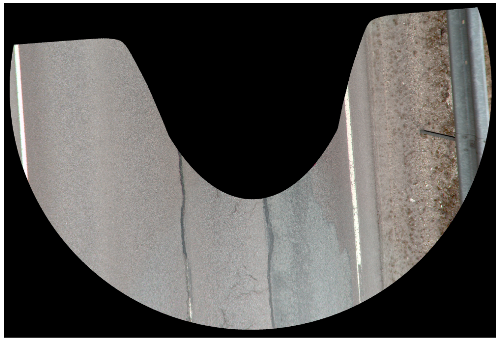
• Inconsistent sharpness across the image. This stemmed from the horizontal placement of some of the Ladybug cameras. Due to the simple laws of optics, road surface gradually loses detail as the distance from the original camera shooting location increases. See Figure 2.
• Inconsistent brightness from image to image. This was related to the availability of light at the moment when an image was taken. Note that the situation has improved considerably not only because of the CMOS sensors of Ladybug 5+, but also because Reach-U Ltd. has instructed the MMSdriver to adjust the shutter speed manually during the data collection if the lighting conditions change on the road to avoid under- or over-exposure.
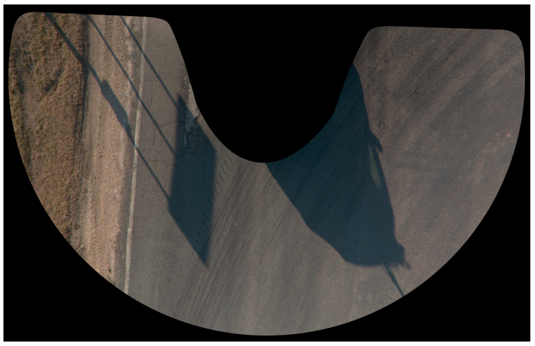
• Comparatively high number of shadows cast by various objects on the road, near the road, by the camera rig, or by the car itself doing the mapping. The intensity of shadows is directly correlated with the availability of light, and their extent is (among other things) dependent on the angle of Sun rays, which is illustrated in Figure 3.

In addition, there were various artifacts found in some images (vehicle fragments, people, etc.). However, there were only a few of these, so in general, they can be treated as statistically irrelevant and ignored.

Inconsistent quality of the images may mislead the ConvNet training [71], and although by forsaking the orthophoto format, we were able to avoid the “stitching seams” among individual orthoframes, the gradual loss of detail as we moved away from the position of the camera still presented a problem. We therefore focused on the sharper part of the orthoframe. The original orthoframe mask was multiplied with a filled circle with a radius of 1500 pixels. The resulting mask (Figure 4) was then used to extract the more detailed part of the orthoframe. As the consecutive orthoframes were overlapping, there was no loss of ground. Note also that in the resulting image, the area that was not road surface became much smaller and was most often present on one side of the road only and could be thus typically separated with a single line (Figure 5). Therefore, the road extraction procedure that was automated in [2] was now delegated to the digitizers (a digitizer in the context of this work refers to a person engaged in digitization of defect information based on the provided orthoframes and initial defect data) who processed the orthoframes as part of the preprocessing step for obtaining more accurate training data for the automatic detector.

Out of 33,288 orthoframes, 20,318 that contained defects in the area of interest were algorithmically picked out for further consideration. Out of this selection, orthoframes with poor lighting conditions, poorly distinguishable defects, or other problems were abandoned after visual inspection. For actual digitization, 1572 orthoframes were used.

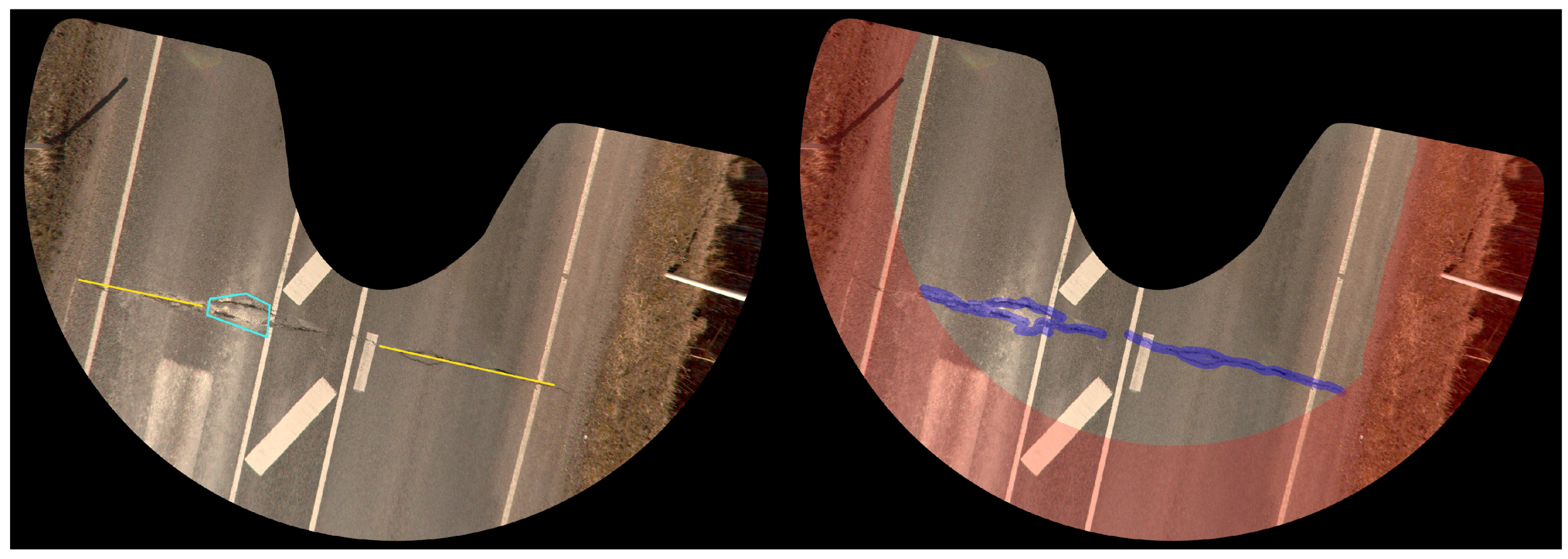
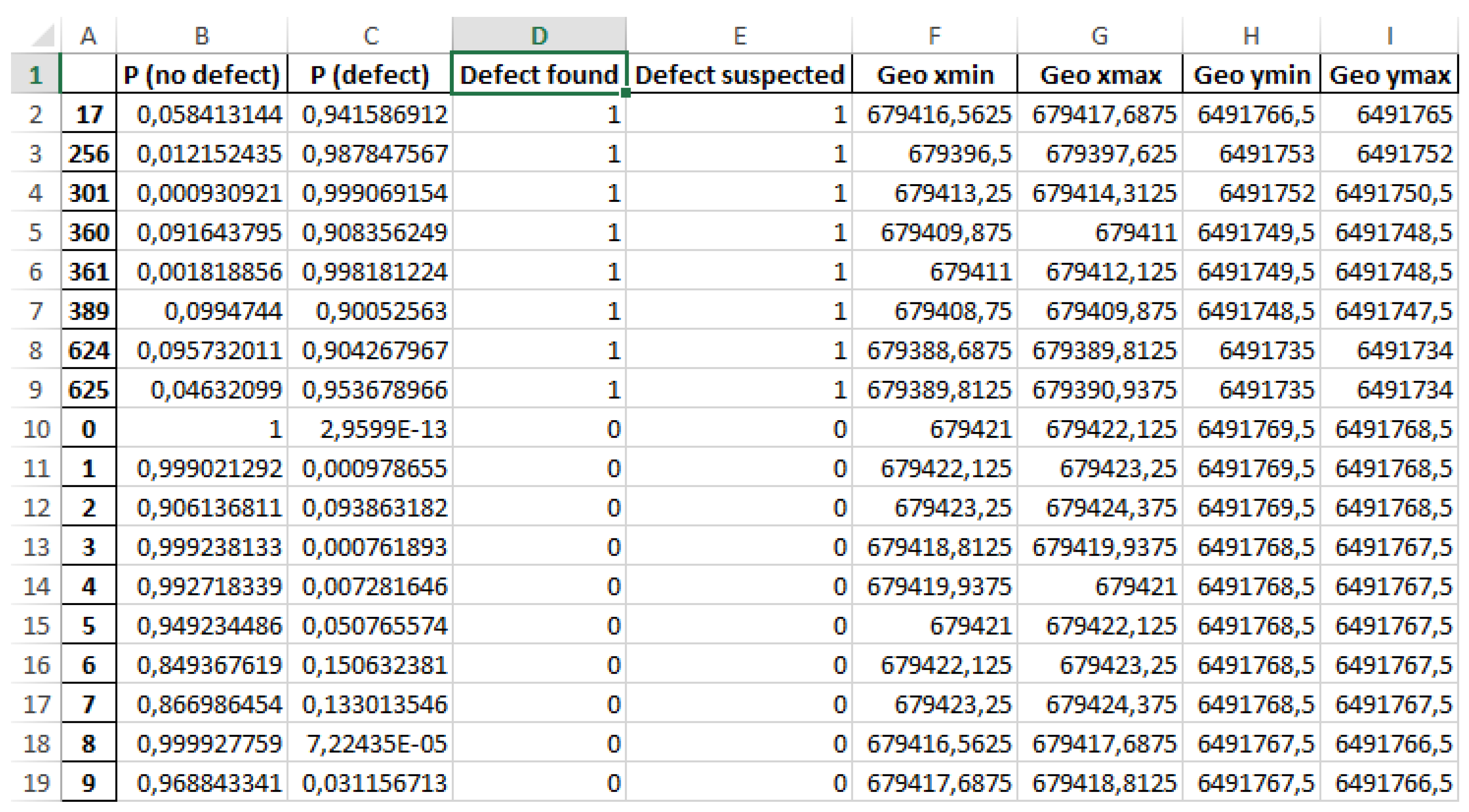
2.2. Pavement Distress Digitization

The defect layer provided by Reach-U Ltd. contained information about the pavement defects listed in

Table 4. Types of pavement defects.

Polyline Defect Types	Polygon Defect Types	Point Defect Types
narrow longitudinal crack	network cracking	pothole
narrow joint reflection crack	patched road
patched road (line)	weathering
transverse cracking
edge defect

based on general polyline, polygon, or point defect types. The number of defects per defect class counted from the orthoframes is given in

Table 5. Distribution of defect classes.

Defect	Count
narrow longitudinal crack	13,475
narrow joint reflection crack	1792
patched road (line)	4108
transverse cracking	7139
edge defect	20,877
network cracking	11,709
patched road	1036
weathering	1240
pothole	32

. The overall number of defects obtained this way (61408) was considerably larger than the actual number of defects (25771) on observed roads because usually, the same defect can be found from up to three consecutive orthoframes.

From the distribution of defect classes, it appeared that the data were imbalanced, i.e., there were too few examples of defects of specific classes for training the convolutional neural network [72]. For this reason, all defects were lumped together, and no attempt was made to train the network to distinguish between individual defect classes, resulting in a binary classification problem.

To visualize pavement distress, e.g., cracks, clearly, it is customary to use very strong illumination while taking the shots with the camera [73]. This was not the case here, and defects could be found in shadowed regions with soft and hard shadows. Defects could be also found near other consistent visual features, e.g., road markings. This will inevitably reduce the accuracy of detection.

Most importantly, defect coordinates in the defect layer were often not very accurately determined (Figure 6, left). This is not critical in the application in which they were used originally and thus not the primary concern of the original digitizers. For machine learning purposes, however, it is highly important that the samples that are exploited for defect recognition depict actual defects and, conversely, that the samples that are supplied for defect-free pavement recognition not contain any defects. To provide this level of accuracy, 1572 selected orthoframes were redigitized yielding 12,728 training samples (6364 for each of two classes).

2.3. Image Partitioning

Since the original images were of high resolution, they were partitioned into smaller fragments that we refer to as segments throughout this paper. The idea was to study the contents of each segment and to determine whether it depicted a pavement defect or not. The total of all of these segments formed the basis for training the artificial neural network.

Segments were extracted automatically from the annotated images described in the previous section. The resulting dataset may also be augmented as needed, i.e., the number of images depicting the defects was artificially increased by applying various transformations to existing images such as translation and rotation; in theory, this should improve the efficiency of the ConvNet training.

The partitioning algorithm extracted the initial segments based on a simple grid also capturing some redundant segments on the edges to ensure maximum coverage of the orthoframe area of interest. Only those segments that fell unto the unmasked area were kept, though there was also the option to ignore segments that were partially masked. The segments were exported into a large number of PNG image files into two folders: defect_0 containing segments that depicted no defects and defect_1 containing segments with pavement defects. The procedure of division into these two classes was carried out based on the defect masks manually obtained via digitization during the preprocessing step, as discussed above.

2.4. Further Data Processing and Augmentation

Previously, it was observed that the neural networks were sensitive to different lighting conditions. Models trained on images in certain types of lighting conditions were unable to generalize well to make unbiased predictions for brighter or darker images. To combat this, we experimented with gamma correction and normalization methods. However, these correction methods might result in a loss of information by intensifying the noise present in the image, which is especially undesirable for inference.

Therefore, image preprocessing methods were abandoned. Instead, training data were augmented by applying a random amount of change to brightness and contrast values. For each new epoch, all the training samples were subject to up to a 35% increase or decrease to both brightness and contrast values. An added benefit of this method was the effective increase in different training samples. Additionally, training data were augmented by random horizontal and vertical flips, as well as random rotations up to ±180 degrees, where the missing pixels were filled by reflecting the border pixels. Various potential outputs of the transformation function can be seen in Figure 7.

2.5. Classification Performance Evaluation

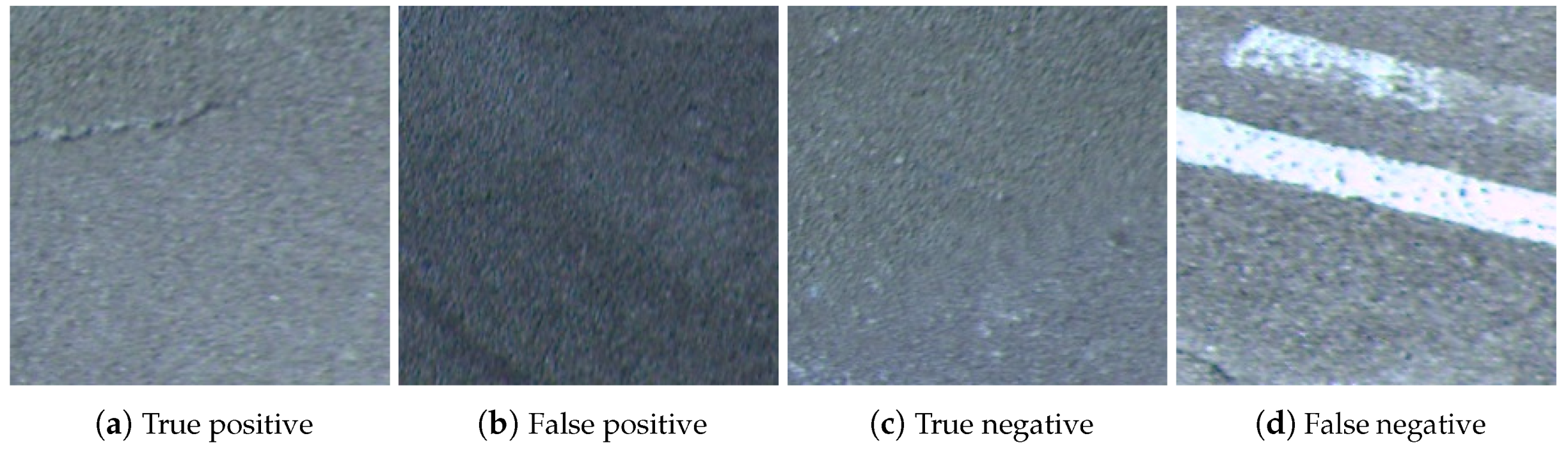
In this work, we were concerned with developing an accurate detector of pavement distress based on image data supplied to it. There were four possible outcomes concerning the judgments of road segments given by the classification system:

• true negative ($TN$): there is no defect, and the system does not detect a defect;
• true positive ($TP$): there is a defect, and the system correctly detects it;
• false negative ($FN$): there is a defect, but the system does not detect it;
• false positive ($FP$): there is no defect, but the system detects a defect.

Based on this, it is possible to impose accuracy criteria for the system, where $TN$, $TP$, $FN$, and $FP$ denote the total counts of the corresponding detection outcomes. First, we argue that the bare accuracy measure given as:

$$\mathrm{Accuracy}=\frac{TP+TN}{TP+TN+FP+FN}$$

(1)

is not as meaningful as the recall and precision measures since it is critical to identify actual defects properly. The recall measure shows the percentage of how many actual defects were detected by the system and is defined as:

$$\mathrm{Recall}=\frac{TP}{TP+FN}$$

(2)

and precision shows the percentage of how many of the detected defects were actual defects and is defined as:

$$\mathrm{Precision}=\frac{TP}{TP+FP}.$$

(3)

We also used the so-called Matthews correlation coefficient (MCC) metric, which is defined as:

$$\mathrm{MCC}=\frac{TP·TN-FP·FN}{\sqrt{(TP+FP)(TP+FN)(TN+FP)(TN+FN)}}$$

(4)

because it provides a more reliable measure in the case of imbalanced data.

Finally, since ConvNets returns probabilities and not discrete values, one must use two threshold values: detection threshold $P_{det}$ and suspicion threshold $P_{sus}$, such that:

$$P\left(\mathrm{defect}\right)⩾P_{det}\Rightarrow \mathrm{defect}\mathrm{is}\mathrm{detected}$$

and

$$P\left(\mathrm{defect}\right)⩾P_{sus}\Rightarrow \mathrm{defect}\mathrm{is}\mathrm{suspected}.$$

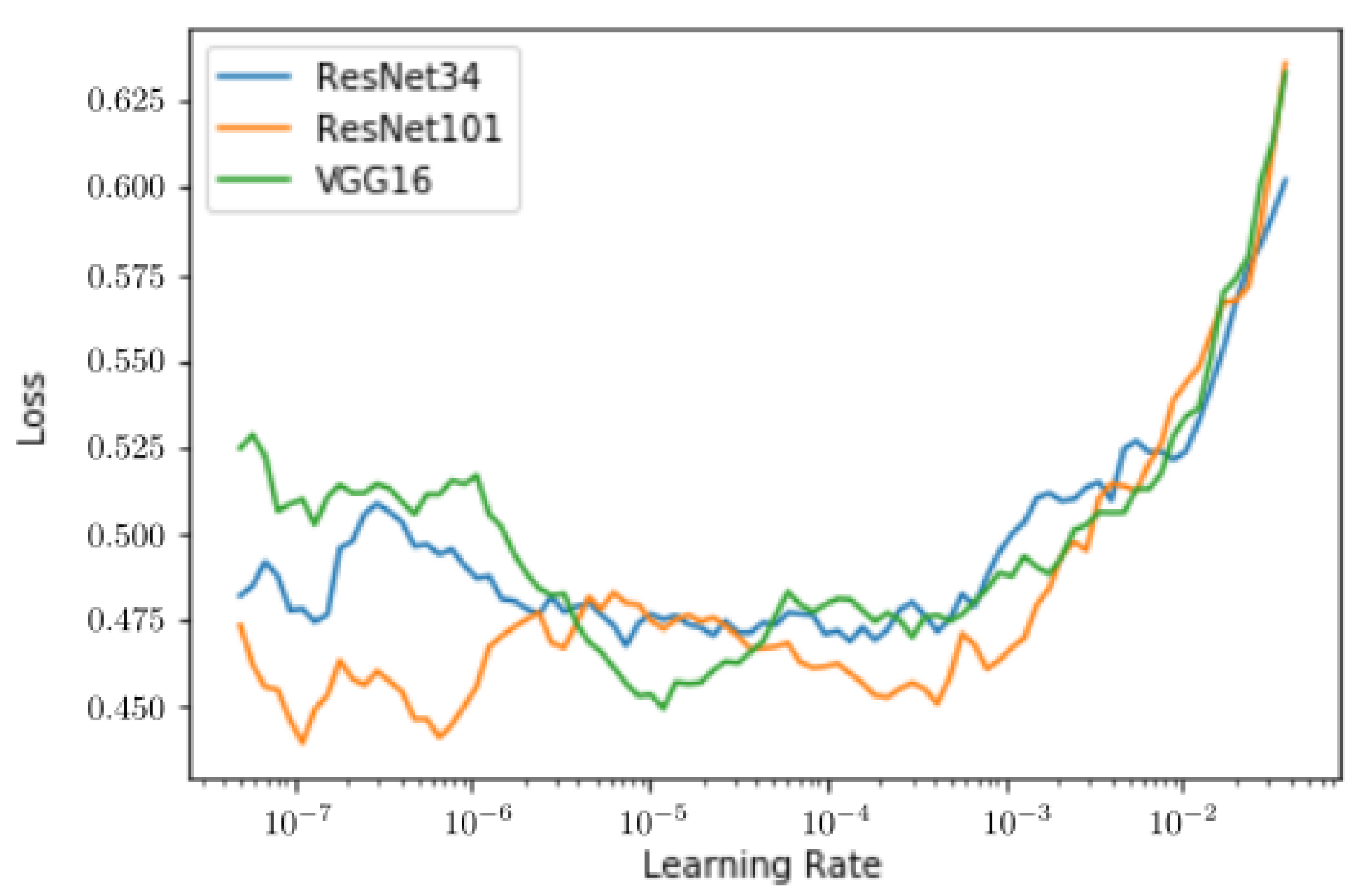
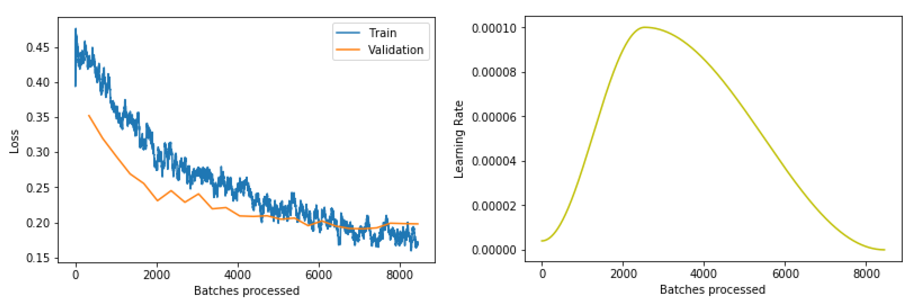
2.6. Deep Neural Networks’ Setup

Convolutional neural networks are deep neural networks specifically tailored for analyzing visual imagery. The major advantage of ConvNets is that they require little preprocessing compared to other image classification algorithms. Three main types of layers that make up ConvNet architectures are convolutional layers, pooling layers, and fully connected layers. The main building block of ConvNets is the convolutional layer.

A convolution is the application of a filter to the layer input that results in a map of activations (feature map), indicating the locations and strength of a detected feature in an input [74]. The convolution is performed by sliding a $K\times K$ convolution filter (kernel) over the input image with a predetermined step size (stride). The innovation of using the convolution operation in a neural network is that the values of the filter are learned during the training of the network. Under stochastic gradient descent, the network is forced to learn to extract features from the input that are most useful for classifying images.

ConvNets usually learn multiple (32–512) filters in parallel for a given input. A filter must have the same number of channels (depth) as the input and can have specific filter values for each of the input channels. Regardless of the depth of the input and depth of the filter, each filter produces a 2D feature map because eventually, the channels are summed together to form one single channel (element-wise addition).

The Rectified Linear Unit (ReLU) is a supplementary step to the convolution operation. Its purpose is to increase the non-linearity in feature maps. The result of the convolution operation is passed through the ReLU activation function so the values in final feature maps are not just the sums, but the ReLU function applied to the sums. The ReLU activation function has rapidly become the default activation function for most types of neural networks. It provides true zero and acts like a linear function for the most part, but is actually a nonlinear function allowing complex relationships in the data to be learned. ReLU is also easy to implement, and networks trained with this activation function avoid the problem of vanishing gradients [75].

The depth of the output of a convolutional layer is determined by the number of filters because each of them creates a distinct feature map. The width and height of the output of a convolutional layer are, on the other hand, determined by the formula:

$$D_o=1+\frac{D_i-K+2P}{S},$$

(5)

where $D_o$ and $D_i$ are the height/length of the output and input, S is the stride, and P is the width of the added border of zeros (zero-padding). Note that commonly, $K=3,P=1,S=1$, and $D_o=D_i$.

Pooling layers do not affect the depth dimension, but perform a downsampling operation along the spatial dimensions (width, height) of the input for the next convolutional layer. The decrease in size leads to less computational overhead for the upcoming layers of the network, works against over-fitting, and improves local translation invariance. Much like the convolution operation, the pooling layer takes a sliding window that is moved in stride across the input and transforms its values into a more representative value by selecting, e.g., the maximum value from the window (max pooling). Contrary to the convolution operation, however, pooling has no trainable parameters, although window (kernel) size and stride must be specified. Commonly, $K=2,S=2$.

Fully-connected layers are ordinary neural network layers that are fully connected with the output of the previous layer and are typically used in the last stages of the ConvNet. They are also used to construct the desired number of nodes in the output layer. A fully connected layer expects a 1D vector of numbers as its input so the 3D output of the final pooling or convolution layer must be flattened into a 1D vector of numbers before it becomes the input to the fully connected layer.

The most common form of a ConvNet architecture stacks a few convolutional layers (CONV), followed by a (optional) pooling layer (POOL), and repeats this pattern until the image has been reduced spatially to a small size. At this point, it is customary to introduce the fully connected layers (FC). The standard final layer for a multiclass classification problem is a fully connected layer with a number of nodes that corresponds to the number of classes and that uses the softmax function as its activation function that converts the numbers into probabilities. The ConvNet architecture thus appears as:

$$\begin{array}{|c|}\hline \mathrm{Input}\phantom{\int }\\ \hline\end{array}\to \begin{array}{|c|}\hline \begin{array}{|c|}\hline \mathrm{CONV}\phantom{\int }\\ \hline\end{array}\times N\to \begin{array}{|c|}\hline \mathrm{POOL}\phantom{\int }\\ \hline\end{array}\\ \hline\end{array}\times M\to \begin{array}{|c|}\hline \mathrm{FC}\phantom{\int }\\ \hline\end{array}\times L\to \begin{array}{|c|}\hline \mathrm{FC}\phantom{\int }\\ \hline\end{array},$$

(6)

where $N\in [1,3),M\ge 0,L\in [0,3)$.

Typically, ConvNets are trained with the stochastic gradient descent, and its weights are updated using the backpropagation method. The objective function to be minimized (loss function) is defined as the cross-entropy between the training data and the network response.

Deep neural networks frequently incorporate a regularization technique called dropout to prevent overfitting [76]. At each training iteration, a neuron is temporarily disabled with probability p (all the inputs and outputs to it will be disabled). The dropped out neurons are resampled with probability p at every training step, so a dropped out neuron at one step can be active at the next one. The hyperparameter p is called the dropout rate, and it is typically a number around 0.5, corresponding to 50% of the neurons being dropped out.

A ConvNet model can be thought as a combination of two components: the feature extraction part and the classification part. The convolution and pooling layers perform feature extraction. The fully connected layers act as a classifier on top of the extracted features and assign a probability for the input image representing a class. The lower layers encode/detect simple structures (colors, edges, and simple shapes), and as we go deeper into the network, the layers build on top of each other and learn to encode more complex patterns.

One of the problems using deep ConvNets is the requirement to have large annotated image datasets. For some domains, obtaining such data can be difficult, time consuming, and costly. To overcome those difficulties, transfer learning can be used by applying the ConvNets pretrained on large datasets (such as VGG-16, AlexNet [77], GoogLeNet [78], and ResNet) to a new classification task. Networks with architectures that perform well on large scale classification tasks such as the ImageNet Large Scale Visual Recognition Challenge (ILSVRC) [79] have been found to be able to generalize to other tasks of image classification by retraining the fully connected layers that are near the output of the network while keeping the feature extraction part of the network with the pretrained weights ([80,81,82]).

In this work, we considered three architectures optimized for the ImageNet dataset for our task of pavement distress detection:

• VGG16 [83], which was the best performing classifier of ILSVRC in 2014 along with GoogLeNet. This architecture has 16 weight layers, 13 of which consist of 3 × 3 convolutional filters with a total of 4224 filters, followed by three fully connected layers of length 4096, 4096, and 1000, respectively. In total, it has 15,252,034 trainable parameters.
• ResNet34 and ResNet101 [84], which introduced residual blocks to the typical ConvNet architecture and won ILSVRC in 2015. The residual block allows connections from earlier preceding convolutional layers, not only the immediately preceding one. This allows deeper models to be trained while also maintaining information only a shallower network would be able to capture [85]. As for the convolutional layers, ResNet follows the design of VGG16 with 3 × 3 convolutional filters, except for the first layer, which has 7 × 7 filters. In our work, ResNet34 had 33 convolutional layers and two fully connected layers of length 1024 and 512 and a total of 21,813,570 trainable parameters. Its deeper counterpart ResNet101 had 100 convolutional layers and two fully connected layers of length 4096 and 512, with a total of 44,608,066 trainable parameters.

3. Experimental Results

3.1. Data Selection

The 1572 selected orthoframes were partitioned into segments each having dimensions of 224 × 224 pixels, which is the size many transfer learning architectures take as a default input [84,86]. Smaller and larger dimensions could also be considered, but there is a trade-off for both of these cases. Smaller segment sizes allowed us to capture more of the road, leaving fewer blind spots. However, it is more difficult to make predictions on smaller segments due to missing context. Conversely, larger segments provide more context for better accuracy, but at the cost of leaving more blind spots at the edge of the road (assuming non-overlapping segments).

In order to classify a segment as defect or not defect, we considered the percentage of defect pixels on the image. If more than 5% of the pixels on a segment were masked by the digitizer, it would be labeled as a defect segment. With this criterion, 15% of all segments would have a defect, and 85% would not. It is known that class imbalance during training reduces the performance of deep neural networks [87]. To balance our dataset, only N non-defect segments were sampled for each orthoframe containing N defect segments. This way, ~8 segments per orthoframe were sampled on average.

For the purposes of neural network training, the obtained 12,728 segments with dimensions 224 × 224 pixels were split into training and validation sets, with the ratio of 0.85 and 0.15, respectively. As is typical for deep learning cases, the training set was used to optimize the parameters of the model with respect to the cross-entropy loss function, and the validation set was used to measure if the model was overfit to the training data.

In addition, a test set consisting of 55 new orthoframes from different roads was used to evaluate how well the model generalized to new conditions. As opposed to the training and validation set, for the test set, we extracted all of the possible segments, so a total of 1007 defect-free and 185 defect segments were obtained.

3.2. Deep Learning

Throughout the process, the Python library PyTorch [88] was used along with fastai [89], which provides a layer of abstraction upon PyTorch to simplify the experimentation process.

In the choice of hyperparameters, a “learning rate range test” was performed, as suggested by L.N. Smith [90,91]. The network was trained for an epoch with a linearly increasing learning rate, while the loss was measured after each processed batch. The maximum learning rate for the given model was then heuristically decided upon such that it was not in the region where the loss had a rising trend (refer to Figure 8). The learning rates chosen can be seen in

Table 6. Hyper-parameters for training the models used in this work.

Model	Base Learning Rate	Maximum Learning Rate for Layer L	Momentum Lower Bound	Momentum Upper Bound	Weight Decay	Batch Size
VGG16	$4.0\times {10}^{-7}$	$1.0\times {10}^{-5}$	0.85	0.95	0.01	32
ResNet34	$3.2\times {10}^{-6}$	$8.0\times {10}^{-5}$	0.85	0.95	0.01	32
ResNet101	$4.0\times {10}^{-5}$	$1.0\times {10}^{-4}$	0.85	0.95	0.01	32

.

For all model architectures, we used the pretrained weights optimized for the ImageNet dataset. Then, all of the layers except for the fully connected layers of length 4096 and 512 respectively were frozen, meaning we did not optimize the convolutional filters. In this configuration, the model was trained for two epochs. This selective freezing of the weights was done to speed up the training and ensure the earlier layers of the pretrained network were subject to less noise. After training for two epochs, all of the model parameters were unfrozen for fine-tuning purposes.

Discriminative fine-tuning was used for further training of the model [92]. The idea was to train the layers towards the output at higher learning rates than the earlier layers. In our case, we used logarithmically stepped learning rates:

$$\eta \left(l\right)=\frac{\eta \left(L\right)}{N}{\left(N{}^{\left(\frac{1}{L-1}\right)}\right)}^{l-1},$$

(7)

where $\eta \left(l\right)$ is the learning rate of the layer l, L is the number of layers, and N is $\frac{\eta \left(L\right)}{\eta \left(1\right)}$, which we chose to be 10. Additionally, the learning rates were cyclical throughout the process, which was shown to speed up the training process [93]. For the optimizer algorithm, we chose to use Adam [94].

The 25 epoch training process can be seen in Figure 9.

It can be observed that throughout the initial epochs, the validation loss was actually lower than the training loss. This can be explained by the fact that the validation data were not subjected to the aggressive brightness and contrast preprocessing. Additionally, the dropout layers were disabled while evaluating the model. After 25 epochs, which corresponded to 8300 training batches in Figure 9, the training loss reached below the validation loss; therefore, in order to prevent overfitting, training was stopped.

3.3. Results

From the tests (the results of which are presented in

Table 7. Performance metrics of the obtained ConvNets computed over the test set discussed in Section 3.1.

Model	Accuracy	Precision	Recall	MCC
VGG16 net fine-tuned	0.95	0.90	0.79	0.82
ResNet34 fine-tuned	0.96	0.92	0.82	0.84
ResNet101 fine-tuned *	0.97	0.90	0.87	0.87

* Validation set figures are $0.96$ for precision and $0.93$ for recall.

), it can be noted that the problem of crack detection benefited from the more sophisticated architecture of ConvNets as the 101 layer ResNet slightly outperformed the 34 layer ResNet. Further inspection of the obtained results revealed that many of the misclassifications were due to our labeling methodology. A manually masked defect at the corner of the image may not have passed the 5% threshold, therefore confusing the classifier (refer to Figure 10d). A few of the false positives were due to miscellaneous shapes on the road, such as tire marks, spills, etc. (refer to Figure 10b). Most of the other misclassifications included segments that were ambiguous due to low image quality and lack of context.

Any trained network can be employed to find and localize the defects from the whole orthoframe. Figure 11 depicts an orthoframe that can be considered highly problematic due to a number of sharp contoured shadows. Yet, the network was able to localize a definite crack on the left side of the image. It also suggested another damaged area on the right where the pavement was apparently problem free, however.

3.4. Software Solution

As a result of this research and development project, a fully-fledged Python software package was developed for Reach-U Ltd. that could be used to generate the data for training and inspect them; annotate (digitize) the images as needed for creating defect masks and also updating the initial image masks; train the deep learning ConvNets and apply them to arbitrary new images. The package comprised back-end functionality in two separate Python libraries and also had graphical user interfaces developed using PyQt5. The intended end-user application entitled nnapply included a graphical user interface and allowed processing arbitrary road images using the trained ConvNets, showing the detected and suspected defects. It also generated a report in Microsoft Excel format. Examples of both types of output from this application are depicted in Figure 11 and Figure 12.

The implementation of the back-end described in [2] is now being updated to use the newly introduced deep learning libraries, but thanks to the proper separation of back- and front-end functionality, this is a relatively straightforward process.

4. Discussion

In this paper, we presented a fully working prototype of a computer vision system designed to detect pavement distress based on orthoframes captured by a mobile mapping system. The prototype has to be tested in the appropriate transportation system analysis environment; therefore, the presently claimed technology readiness level (TRL) is four (i.e., tested in a laboratory environment).

Further items for discussion are presented next:

• In [2], it was claimed that detection of shadow regions in the orthoframe is a critical component of the complete pavement distress detection system. However, our current tests did not completely confirm this as the system seemed to be robust to such visual artifacts. Hard shadows from tree branches still presented a problem, however, as they resembled pavement cracks.
• Ensemble classifiers were not introduced in this work as acceptable performance was obtained without complicating the system architecture. An attempt to make the detector context sensitive, i.e., use progressive zoom where a defect was suspected in the orthoframe, was considered as a possible next step in improving detection performance especially as a countermeasure for hard, fine-detail shadows.
• Data augmentation was updated to include orthoframe segment exposure variation and apparently led to improved generalization ability of the resulting ConvNet.
• Finally, the current classifier could only be regarded as a detector since the predictions about orthoframe segments were essentially binary, whether a defect was detected or not, with the additional possibility to consider suspected defects. In the future, a more advanced segmentation feature can be implemented whereby different types of defects will have related ground truth information provided by means of manual annotation for which the corresponding software package was also developed as part of this effort. In this case, however, as was shown previously, the issue of imbalanced data will have to be solved.

5. Conclusions

In the present work, a deep learning convolutional neural network model based on several existing architectures of image classifiers was obtained using fine-tuning. The data for fine-tuning were carefully selected from thousands of existing orthoframes freshly provided by the company and having better image quality compared to the images used in [2].

The manual preprocessing step that included digitizing the orthoframes, i.e., manually painting defect masks and updating the road mask by eliminating image areas with poor sharpness and also areas outside the pavement part, while time consuming and tedious, was proven to be critical for the success of the implementation of the detector. In previous work, we used the data provided by the company for generating ground truth information. However, it must be taken into account that the internal purposes of digitization in the company were different, so pixel annotation accuracy was not the most important factor. Therefore, to ensure that the detection model was developed based on relevant information, a more accurate localization of defects had to be introduced. Due to this redundant approach in annotating images, the proposed solution while not completely foolproof should be fairly robust with respect to annotation mistakes, at least from the point of view of visual inspection.

Furthermore, data augmentation was proven to be useful to combat differing lighting conditions that still presented a challenge while analyzing the image. The next step for data augmentation is the implementation of distortion tuning [71].

Instead of attempting to train convolutional neural networks from scratch, we only considered pretrained neural networks in this work. The reason for this was that significantly better results were obtained with pretrained networks compared to the results reported in [2], and therefore, using simpler network structures was not considered a benefit. Indeed, precision and recall metrics increased from 0.22 and 0.35, respectively, to 0.90 and 0.87. This was a significant improvement and was very likely related to several factors, including better quality orthoframes, using only sharp image areas, and manually digitizing the images, annotating defects and updating pavement masks as needed. The latter also contributed to solving the problem that appeared in [2] where the majority of false positive detections was due to the classifier incorrectly identifying road edges as pavement distress.

Finally, the software package proposed to the company was updated and also included an efficient image annotation tool tailored to the specific purpose of preparing higher quality ground truth files for defect detection and pavement area extraction. Although a different deep learning backend was used (PyTorch and FastAI instead of TensorFlow and Keras), the software is easy to update and hence it will soon be ready for deployment, further testing, and its eventual application for improving highway road pavement conditions.

References

1. Mohan, A.; Poobal, S. Crack detection using image processing: A critical review and analysis. Alex. Eng. J. 2018, 57, 787–798. [Google Scholar] [CrossRef]
2. Tepljakov, A.; Riid, A.; Pihlak, R.; Vassiljeva, K.; Petlenkov, E. Deep Learning for Detection of Pavement Distress using Nonideal Photographic Images. In Proceedings of the 42nd International Conference on Telecommunications and Signal Processing, Budapest, Hungary, 1 July 2019. [Google Scholar] [CrossRef]
3. Yandell, W.; Pham, T. A fuzzy-control procedure for predicting fatigue crack initiation in asphaltic concrete pavements. In Proceedings of the 1994 IEEE 3rd International Fuzzy Systems Conference, Orlando, FL, USA, 26–29 June 1994; pp. 1057–1062. [Google Scholar] [CrossRef]
4. Tsubota, T.; Yoshii, T.; Shirayanagi, H.; Kurauchi, S. Effect of Pavement Conditions on Accident Risk in Rural Expressways. In Proceedings of the IEEE Conference on Intelligent Transportation Systems, Maui, HI, USA, 4–7 November 2018; pp. 3613–3618. [Google Scholar] [CrossRef]
5. Tsukamoto, A.; Hato, T.; Adachi, S.; Oshikubo, Y.; Cheng, W.; Enpuku, K.; Tsukada, K.; Tanabe, K. Eddy Current Testing System Using HTS-SQUID with External Pickup Coil Made of HTS Wire. IEEE Trans. Appl. Supercond. 2017, 27. [Google Scholar] [CrossRef]
6. Wang, M.; Sun, M.; Zhang, X.; Wang, Y.; Li, J. Mechanical behaviors of the thin-walled SHCC pipes under compression. In Proceedings of the ICTIS 2015—3rd International Conference on Transportation Information and Safety, Wuhan, China, 25–28 June 2015; pp. 797–801. [Google Scholar] [CrossRef]
7. Jenkins, M.D.; Carr, T.A.; Iglesias, M.I.; Buggy, T.; Morison, G. A deep convolutional neural network for semantic pixel-wise segmentation of road and pavement surface cracks. In Proceedings of the European Signal Processing Conference, Rome, Italy, 3–7 September 2018; pp. 2120–2124. [Google Scholar] [CrossRef]
8. Konig, J.; David Jenkins, M.; Barrie, P.; Mannion, M.; Morison, G. A Convolutional Neural Network for Pavement Surface Crack Segmentation Using Residual Connections and Attention Gating. In Proceedings of the 2019 IEEE International Conference on Image Processing (ICIP), Taipei, Taiwan, 22–25 September 2019; pp. 1460–1464. [Google Scholar] [CrossRef]
9. Mandal, V.; Uong, L.; Adu-Gyamfi, Y. Automated Road Crack Detection Using Deep Convolutional Neural Networks. In Proceedings of the 2018 IEEE International Conference on Big Data, Seattle, WA, USA, 10–13 December 2018; Institute of Electrical and Electronics Engineers Inc.: Piscataway, NJ, USA, 2019; pp. 5212–5215. [Google Scholar] [CrossRef]
10. Nie, M.; Wang, K. Pavement Distress Detection Based on Transfer Learning. In Proceedings of the 2018 5th International Conference on Systems and Informatics, Nanjing, China, 10–12 November 2018; Institute of Electrical and Electronics Engineers Inc.: Piscataway, NJ, USA, 2019; pp. 435–439. [Google Scholar] [CrossRef]
11. Zhang, L.; Yang, F.; Daniel Zhang, Y.; Zhu, Y.J. Road crack detection using deep convolutional neural network. In Proceedings of the International Conference on Image Processing, Phoenix, AZ, USA, 25–28 September 2016; pp. 3708–3712. [Google Scholar] [CrossRef]
12. Cafiso, S.; D’Agostino, C.; Delfino, E.; Montella, A. From manual to automatic pavement distress detection and classification. In Proceedings of the 2017 5th IEEE International Conference on Models and Technologies for Intelligent Transportation Systems (MT-ITS), Naples, Italy, 26–28 June 2017; pp. 433–438. [Google Scholar] [CrossRef]
13. Wang, X.; Hu, Z. Grid-based pavement crack analysis using deep learning. In Proceedings of the 2017 4th International Conference on Transportation Information and Safety (ICTIS), Banff, AB, Canada, 8–10 August 2017; pp. 917–924. [Google Scholar] [CrossRef]
14. Yusof, N.A.; Osman, M.K.; Noor, M.H.; Ibrahim, A.; Tahir, N.M.; Yusof, N.M. Crack detection and classification in asphalt pavement images using deep convolution neural network. In Proceedings of the 8th IEEE International Conference on Control System, Computing and Engineering, Penang, Malaysia, 23–25 November 2018; Institute of Electrical and Electronics Engineers Inc.: Piscataway, NJ, USA, 2019; pp. 227–232. [Google Scholar] [CrossRef]
15. Le Bastard, C.; Pan, J.; Wang, Y.; Sun, M.; Todkar, S.S.; Baltazart, V.; Pinel, N.; Ihamouten, A.; Derobert, X.; Bourlier, C. A Linear Prediction and Support Vector Regression-Based Debonding Detection Method Using Step-Frequency Ground Penetrating Radar. IEEE Geosci. Remote. Sens. Lett. 2019, 16, 367–371. [Google Scholar] [CrossRef]
16. Salari, E.; Ouyang, D. An image-based pavement distress detection and classification. In Proceedings of the IEEE International Conference on Electro Information Technology, Indianapolis, IN, USA, 6–8 May 2012. [Google Scholar] [CrossRef]
17. Savant Todkar, S.; Le Bastard, C.; Baltazart, V.; Ihamouten, A.; Dérobert, X. Comparative study of classification algorithms to detect interlayer debondings within pavement structures from Step-frequency radar data. In Proceedings of the International Geoscience and Remote Sensing Symposium (IGARSS), Valencia, Spain, 22–27 July 2018; pp. 6820–6823. [Google Scholar] [CrossRef]
18. Todkar, S.S.; Le Bastard, C.; Ihamouten, A.; Baltazart, V.; Dérobert, X.; Fauchard, C.; Guilbert, D.; Bosc, F. Detection of debondings with ground penetrating radar using a machine learning method. In Proceedings of the 2017 9th International Workshop on Advanced Ground Penetrating Radar, Edinburgh, UK, 28–30 June 2017. [Google Scholar] [CrossRef]
19. Aggarwal, P. Predicting dynamic modulus for bituminous concrete using support vector machine. In Proceedings of the 2017 International Conference on Infocom Technologies and Unmanned Systems: Trends and Future Directions, Dubai, UAE, 18–20 December 2017; Institute of Electrical and Electronics Engineers Inc.: Piscataway, NJ, USA, 2018; pp. 751–755. [Google Scholar] [CrossRef]
20. Ai, D.; Jiang, G.; Siew Kei, L.; Li, C. Automatic Pixel-Level Pavement Crack Detection Using Information of Multi-Scale Neighborhoods. IEEE Access 2018, 6, 24452–24463. [Google Scholar] [CrossRef]
21. Brayan, B.A.; Bladimir, B.C.; Sandra, N.R. Pavement and base layers local thickness estimation using computer vision. In Proceedings of the 2015 10th Colombian Computing Conference, Bogota, Colombia, 21–25 September 2015; pp. 324–330. [Google Scholar] [CrossRef]
22. Hassan, N.; Mathavan, S.; Kamal, K. Road crack detection using the particle filter. In Proceedings of the 2017 23rd IEEE International Conference on Automation and Computing: Addressing Global Challenges through Automation and Computing, Huddersfield, UK, 7–8 September 2017. [Google Scholar] [CrossRef]
23. Salman, M.; Mathavan, S.; Kamal, K.; Rahman, M. Pavement crack detection using the Gabor filter. In Proceedings of the 16th International IEEE Conference on Intelligent Transportation Systems (ITSC 2013), The Hague, The Netherlands, 6–9 October 2013; pp. 2039–2044. [Google Scholar] [CrossRef]
24. Strisciuglio, N.; Azzopardi, G.; Petkov, N. Robust Inhibition-Augmented Operator for Delineation of Curvilinear Structures. IEEE Trans. Image Process. 2019, 28, 5852–5866. [Google Scholar] [CrossRef] [PubMed]
25. Zhu, Q. Pavement crack detection algorithm Based on image processing analysis. In Proceedings of the 2016 8th International Conference on Intelligent Human-Machine Systems and Cybernetics, Hangzhou, China, 27–28 August 2016; Volume 1, pp. 15–18. [Google Scholar] [CrossRef]
26. Qian, B.; Tang, Z.; Xu, W. Pavement crack detection based on improved tensor voting. In Proceedings of the 9th International Conference on Computer Science and Education, Vancouver, BC, Canada, 22–24 August 2014; pp. 397–402. [Google Scholar] [CrossRef]
27. Quan, Y.; Sun, J.; Zhang, Y.; Zhang, H. The Method of the Road Surface Crack Detection by the Improved Otsu Threshold. In Proceedings of the 2019 IEEE International Conference on Mechatronics and Automation (ICMA), Tianjin, China, 4–7 August 2019; pp. 1615–1620. [Google Scholar] [CrossRef]
28. Ahmed, N.B.C.; Lahouar, S.; Souani, C.; Besbes, K. Automatic crack detection from pavement images using fuzzy thresholding. In Proceedings of the 2017 International Conference on Control, Automation and Diagnosis, Hammamet, Tunisia, 19–21 January 2017; pp. 528–533. [Google Scholar] [CrossRef]
29. Akagic, A.; Buza, E.; Omanovic, S.; Karabegovic, A. Pavement crack detection using Otsu thresholding for image segmentation. In Proceedings of the 2018 41st International Convention on Information and Communication Technology, Electronics and Microelectronics, Opatija, Croatia, 21–25 May 2018; pp. 1092–1097. [Google Scholar] [CrossRef]
30. Sun, Z.; Li, W.; Sha, A. Automatic pavement cracks detection system based on visual studio C++ 6.0. In Proceedings of the 2010 6th International Conference on Natural Computation, Yantai, China, 10–12 August 2010; Volume 4, pp. 2016–2019. [Google Scholar] [CrossRef]
31. Amhaz, R.; Chambon, S.; Idier, J.; Baltazart, V. A new minimal path selection algorithm for automatic crack detection on pavement images. In Proceedings of the 2014 IEEE International Conference on Image Processing, Paris, France, 27–30 October 2014; pp. 788–792. [Google Scholar] [CrossRef] [Green Version]
32. Baltazart, V.; Nicolle, P.; Yang, L. Ongoing Tests and Improvements of the MPS algorithm for the automatic crack detection within grey level pavement images. In Proceedings of the 25th European Signal Processing Conference, Kos, Greece, 28 August–2 September 2017; pp. 2016–2020. [Google Scholar] [CrossRef] [Green Version]
33. Chatterjee, A.; Tsai, Y.C. A fast and accurate automated pavement crack detection algorithm. In Proceedings of the European Signal Processing Conference. European Signal Processing Conference, Rome, Italy, 3–7 September 2018; pp. 2140–2144. [Google Scholar] [CrossRef]
34. Zou, Q.; Li, Q.; Zhang, F.; Xiong Qian Wang, Z.; Wang, Q. Path voting based pavement crack detection from laser range images. In Proceedings of the International Conference on Digital Signal Processing, DSP, Beijing, China, 16–18 October 2016; pp. 432–436. [Google Scholar] [CrossRef]
35. Dabbiru, L.; Wei, P.; Harsh, A.; White, J.; Ball, J.E.; Aanstoos, J.; Donohoe, P.; Doyle, J.; Jackson, S.; Newman, J. Runway assessment via remote sensing. In Proceedings of the 2015 IEEE Applied Imagery Pattern Recognition Workshop, Washington, DC, USA, 13–15 October 2015; Institute of Electrical and Electronics Engineers Inc.: Piscataway, NJ, USA, 2016. [Google Scholar] [CrossRef]
36. Pudova, N.; Shirobokov, M.; Kuvaldin, A. Application of the Attribute Analysis for Interpretation of GPR Survey Data. In Proceedings of the 2018 17th International Conference on Ground Penetrating Radar, Rapperswil, Switzerland, 18–21 June 2018. [Google Scholar] [CrossRef]
37. Yi, L.; Zou, L.; Sato, M. A simplified velocity estimation method for monitoring the damaged pavement by a multistatic GPR system YAKUMO. In Proceedings of the 2018 17th International Conference on Ground Penetrating Radar, Rapperswil, Switzerland, 18–21 June 2018. [Google Scholar] [CrossRef]
38. Li, Q.; Zhang, D.; Zou, Q.; Lin, H. 3D Laser imaging and sparse points grouping for pavement crack detection. In Proceedings of the 25th European Signal Processing Conference, Kos, Greece, 28 August–2 September 2017; pp. 2036–2040. [Google Scholar] [CrossRef] [Green Version]
39. Medina, R.; Llamas, J.; Zalama, E.; Gomez-Garcia-Bermejo, J. Enhanced automatic detection of road surface cracks by combining 2D/3D image processing techniques. In Proceedings of the 2014 IEEE International Conference on Image Processing, Paris, France, 27–30 October 2014; pp. 778–782. [Google Scholar] [CrossRef]
40. Moazzam, I.; Kamal, K.; Mathavan, S.; Usman, S.; Rahman, M. Metrology and visualization of potholes using the Microsoft Kinect sensor. In Proceedings of the IEEE Conference on Intelligent Transportation Systems, Hague, The Netherlands, 6–9 October 2013; pp. 1284–1291. [Google Scholar] [CrossRef]
41. Ul Haq, M.U.; Ashfaque, M.; Mathavan, S.; Kamal, K.; Ahmed, A. Stereo-Based 3D Reconstruction of Potholes by a Hybrid, Dense Matching Scheme. IEEE Sens. J. 2019, 19, 3807–3817. [Google Scholar] [CrossRef]
42. Yu, Y.; Li, J.; Guan, H.; Wang, C. 3D crack skeleton extraction from mobile LiDAR point clouds. In Proceedings of the International Geoscience and Remote Sensing Symposium (IGARSS), Quebec City, QC, Canada, 13–18 July 2014; pp. 914–917. [Google Scholar] [CrossRef]
43. Zhang, Z.; Cheng, M.; Chen, X.; Zhou, M.; Chen, Y.; Li, J.; Nie, H. Turning mobile laser scanning points into 2D/3D on-road object models: Current status. In Proceedings of the International Geoscience and Remote Sensing Symposium (IGARSS), Milan, Italy, 26–31 July 2015; pp. 3524–3527. [Google Scholar] [CrossRef]
44. Zhang, Y.; Chen, C.; Wu, Q.; Lu, Q.; Zhang, S.; Zhang, G.; Yang, Y. A kinect-based approach for 3D pavement surface reconstruction and cracking recognition. IEEE Trans. Intell. Transp. Syst. 2018, 19, 3935–3946. [Google Scholar] [CrossRef]
45. Zhang, B.; Liu, X. Intelligent Pavement Damage Monitoring Research in China. IEEE Access 2019, 7, 45891–45897. [Google Scholar] [CrossRef]
46. Ziqiang, C.; Haihui, L.; Jiankang, Z. Research of the algorithm calculating the length of bridge crack based on stereo vision. In Proceedings of the 2017 4th International Conference on Systems and Informatics, Hangzhou, China, 11–13 November 2017; Institute of Electrical and Electronics Engineers Inc.: Piscataway, NJ, USA, 2018; pp. 210–214. [Google Scholar] [CrossRef]
47. Fedele, R.; Della Corte, F.G.; Carotenuto, R.; Praticò, F.G. Sensing road pavement health status through acoustic signals analysis. In Proceedings of the 13th Conference on PhD Research in Microelectronics and Electronics, Giardini Naxos, Italy, 12–15 June 2017; pp. 165–168. [Google Scholar] [CrossRef]
48. Uus, A.; Liatsis, P.; Nardoni, G.; Rahman, E. Optimisation of transducer positioning in air-coupled ultrasound inspection of concrete/asphalt structures. In Proceedings of the 2015 22nd International Conference on Systems, Signals and Image Processing, London, UK, 10–12 September 2015; pp. 309–312. [Google Scholar] [CrossRef]
49. Pan, Y.; Zhang, X.; Cervone, G.; Yang, L. Detection of Asphalt Pavement Potholes and Cracks Based on the Unmanned Aerial Vehicle Multispectral Imagery. IEEE J. Sel. Top. Appl. Earth Obs. Remote. Sens. 2018, 1–12. [Google Scholar] [CrossRef]
50. Choi, J.; Zhu, L.; Kurosu, H. Detection of cracks in paved road surface using laser scan image data. In Proceedings of the International Archives of the Photogrammetry, Remote Sensing and Spatial Information Sciences Congress (XXIII ISPRS), Prague, Czech Republic, 12–19 July 2016; Volume XLI-B1, pp. 559–562. [Google Scholar] [CrossRef]
51. Eisenbach, M.; Stricker, R.; Seichter, D.; Amende, K.; Debes, K.; Sesselmann, M.; Ebersbach, D.; Stoeckert, U.; Gross, H. How to get pavement distress detection ready for deep learning? A systematic approach. In Proceedings of the 2017 International Joint Conference on Neural Networks (IJCNN), Anchorage, AK, USA, 14–19 May 2017; pp. 2039–2047. [Google Scholar] [CrossRef]
52. Kapela, R.; Śniatała, P.; Turkot, A.; Rybarczyk, A.; Pożarycki, A.; Rydzewski, P.; Wyczałek, M.; Błoch, A. Asphalt surfaced pavement cracks detection based on histograms of oriented gradients. In Proceedings of the 2015 22nd International Conference Mixed Design of Integrated Circuits Systems (MIXDES), Torun, Poland, 25–27 June 2015; pp. 579–584. [Google Scholar] [CrossRef]
53. Wang, C.; Sha, A.; Sun, Z. Pavement Crack Classification based on Chain Code. In Proceedings of the 2010 Seventh International Conference on Fuzzy Systems and Knowledge Discovery (FSKD 2010), Yantai, China, 10–12 August 2010; pp. 593–597. [Google Scholar] [CrossRef]
54. Yu, X.; Salari, E. Pavement pothole detection and severity measurement using laser imaging. In Proceedings of the IEEE International Conference on Electro Information Technology, Mankato, MN, USA, 15–17 May 2011. [Google Scholar] [CrossRef]
55. Gopalakrishnan, K.; Khaitan, S.K.; Choudhary, A.; Agrawal, A. Deep Convolutional Neural Networks with transfer learning for computer vision-based data-driven pavement distress detection. Constr. Build. Mater. 2017, 157, 322–330. [Google Scholar] [CrossRef]
56. Otsu, N. A Threshold Selection Method from Gray-Level Histograms. IEEE Trans. Syst. Man, Cybern. 1979, 9, 62–66. [Google Scholar] [CrossRef] [Green Version]
57. Oliveira, H.; Correia, P. CrackIT—An image processing toolbox for crack detection and characterization. In Proceedings of the IEEE International Conf. on Image Processing—ICIP, Paris, France, 27–30 October 2014; pp. 798–802. [Google Scholar] [CrossRef]
58. Li, L.; Sun, L.; Ning, G.; Tan, S. Automatic Pavement Crack Recognition Based on BP Neural Network. Promet Traffic Transp. 2014, 26, 11–22. [Google Scholar] [CrossRef] [Green Version]
59. Zhang, D.; Li, Q.; Chen, Y.; Cao, M.; He, L.; Zhang, B. An efficient and reliable coarse-to-fine approach for asphalt pavement crack detection. Image Vis. Comput. 2017, 57, 130–146. [Google Scholar] [CrossRef]
60. Wu, G.; Sun, X.; Zhou, L.; Zhang, H.; Pu, J. Research on Morphological Wavelet Operator for Crack Detection of Asphalt Pavement. In Proceedings of the 2016 IEEE International Conference on Information and Automation, Ningbo, China, 1–3 August 2016; pp. 1573–1577. [Google Scholar] [CrossRef]
61. Zalama, E.; Gómez-Garcà a-Bermejo, J.; Medina, R.; Llamas, J. Road Crack Detection Using Visual Features Extracted by Gabor Filters. Comput.-Aided Civ. Infrastruct. Eng. 2014, 29, 342–358. [Google Scholar] [CrossRef]
62. Oliveira, H.; Caeiro, J.; Correia, P.L. Accelerated unsupervised filtering for the smoothing of road pavement surface imagery. In Proceedings of the 2014 22nd European Signal Processing Conference (EUSIPCO), Lisbon, Portugal, 1–5 September 2014; pp. 2465–2469. [Google Scholar]
63. Quintana, M.; Torres, J.; Menéndez, J.M. A Simplified Computer Vision System for Road Surface Inspection and Maintenance. IEEE Trans. Intell. Transp. Syst. 2016, 17, 608–619. [Google Scholar] [CrossRef] [Green Version]
64. Schlotjes, M.R.; Burrow, M.P.N.; Evdorides, H.T.; Henning, T.F.P. Using support vector machines to predict the probability of pavement failure. Proc. Inst. Civ. Eng. Transp. 2015, 168, 212–222. [Google Scholar] [CrossRef] [Green Version]
65. Koch, C.; Georgieva, K.; Kasireddy, V.; Akinci, B.; Fieguth, P. A review on computer vision based defect detection and condition assessment of concrete and asphalt civil infrastructure. Adv. Eng. Inform. 2015, 29, 196–210, Infrastructure Computer Vision. [Google Scholar] [CrossRef] [Green Version]
66. Doulamis, A.; Doulamis, N.; Protopapadakis, E.; Voulodimos, A. Combined Convolutional Neural Networks and Fuzzy Spectral Clustering for Real Time Crack Detection in Tunnels. In Proceedings of the 2018 25th IEEE International Conference on Image Processing (ICIP), Athens, Greece, 7–10 October 2018; pp. 4153–4157. [Google Scholar] [CrossRef]
67. Yang, F.; Zhang, L.; Yu, S.; Prokhorov, D.; Mei, X.; Ling, H. Feature Pyramid and Hierarchical Boosting Network for Pavement Crack Detection. IEEE Trans. Intell. Transp. Syst. 2019, 1–11. [Google Scholar] [CrossRef] [Green Version]
68. Redmon, J.; Farhadi, A. YOLO9000: Better, Faster, Stronger. arXiv 2016, arXiv:1612.08242. [Google Scholar]
69. Ronneberger, O.; Fischer, P.; Brox, T. U-Net: Convolutional Networks for Biomedical Image Segmentation. In Proceedings of the Medical Image Computing and Computer-Assisted Intervention—MICCAI 2015, Munich, Germany, 5–9 October 2015; pp. 234–241. [Google Scholar] [CrossRef] [Green Version]
70. Zakeri, H.; Nejad, F.M.; Fahimifar, A.; Torshizi, A.D.; Zarandi, M.H.F. A multi-stage expert system for classification of pavement cracking. In Proceedings of the 2013 Joint IFSA World Congress and NAFIPS Annual Meeting (IFSA/NAFIPS), Edmonton, AB, Canada, 24–28 June 2013; pp. 1125–1130. [Google Scholar] [CrossRef]
71. Dodge, S.; Karam, L. A Study and Comparison of Human and Deep Learning Recognition Performance under Visual Distortions. In Proceedings of the 2017 26th International Conference on Computer Communication and Networks (ICCCN), Vancouver, BC, Canada, 31 July–3 August 2017. [Google Scholar] [CrossRef] [Green Version]
72. Khan, S.H.; Hayat, M.; Bennamoun, M.; Sohel, F.A.; Togneri, R. Cost-Sensitive Learning of Deep Feature Representations From Imbalanced Data. IEEE Trans. Neural Networks Learn. Syst. 2018, 29, 3573–3587. [Google Scholar] [CrossRef]
73. Coenen, T.B.J.; Golroo, A. A review on automated pavement distress detection methods. Cogent Eng. 2017, 4. [Google Scholar] [CrossRef]
74. Brownlee, J. Deep Learning for Computer Vision: Image Classification, Object Detection, and Face Recognition in Python; Machine Learning Mastery: Vermont, Australia, 2019. [Google Scholar]
75. Glorot, X.; Bordes, A.; Bengio, Y. Deep Sparse Rectifier Neural Networks. In Proceedings of the Fourteenth International Conference on Artificial Intelligence and Statistics, Fort Lauderdale, FL, USA, 11–13 April 2011; Gordon, G., Dunson, D., Dudík, M., Eds.; Proceedings of Machine Learning Research. PMLR: Fort Lauderdale, FL, USA, 2011; Volume 15, pp. 315–323. [Google Scholar]
76. Krizhevsky, A.; Sutskever, I.; Hinton, G.E. ImageNet classification with deep convolutional neural networks. Commun. ACM 2017, 60, 84–90. [Google Scholar] [CrossRef]
77. Krizhevsky, A.; Sutskever, I.; Hinton, G.E. Imagenet classification with deep convolutional neural networks. In Proceedings of the Advances in Neural Information Processing Systems (NIPS), Lake Tahoe, NV, USA, 3–8 December 2012; pp. 1097–1105. [Google Scholar]
78. Szegedy, C.; Liu, W.; Jia, Y.; Sermanet, P.; Reed, S.; Anguelov, D.; Erhan, D.; Vanhoucke, V.; Rabinovich, A. Going Deeper with Convolutions. In Proceedings of the 2015 IEEE Conference on Computer Vision and Pattern Recognition (CVPR), Boston, MA, USA, 7–12 June 2015. [Google Scholar]
79. Russakovsky, O.; Deng, J.; Su, H.; Krause, J.; Satheesh, S.; Ma, S.; Huang, Z.; Karpathy, A.; Khosla, A.; Bernstein, M.; et al. ImageNet Large Scale Visual Recognition Challenge. Available online: http://arxiv.org/abs/1409.0575v3 (accessed on 15 October 2019).
80. Tajbakhsh, N.; Shin, J.Y.; Gurudu, S.R.; Hurst, R.T.; Kendall, C.B.; Gotway, M.B.; Liang, J. Convolutional Neural Networks for Medical Image Analysis: Full Training or Fine Tuning? IEEE Trans. Med Imaging 2016, 35, 1299–1312. [Google Scholar] [CrossRef] [PubMed]
81. Rosebrock, A. Deep Learning for Computer Vision; PyImageSearch: Columbia, SC, USA, 2017. [Google Scholar]
82. Stricker, R.; Eisenbach, M.; Sesselmann, M.; Debes, K.; Gross, H. Improving Visual Road Condition Assessment by Extensive Experiments on the Extended GAPs Dataset. In Proceedings of the 2019 International Joint Conference on Neural Networks (IJCNN), Budapest, Hungary, 14–19 July 2019; pp. 1–8. [Google Scholar] [CrossRef]
83. Simonyan, K.; Zisserman, A. Very Deep Convolutional Networks for Large-Scale Image Recognition. Available online: http://arxiv.org/abs/1409.1556v6 (accessed on 15 October 2019).
84. He, K.; Zhang, X.; Ren, S.; Sun, J. Deep Residual Learning for Image Recognition. Available online: http://arxiv.org/abs/1512.03385v1 (accessed on 15 October 2019).
85. Zhang, A.; Lipton, Z.C.; Li, M.; Smola, A.J. Dive into Deep Learning. 2019. Available online: http://www.d2l.ai (accessed on 15 October 2019).
86. Krizhevsky, A.; Sutskever, I.; Hinton, G.E. ImageNet Classification with Deep Convolutional Neural Networks. In Advances in Neural Information Processing Systems 25; Pereira, F., Burges, C.J.C., Bottou, L., Weinberger, K.Q., Eds.; Curran Associates, Inc.: Red Hook, NY, USA, 2012; pp. 1097–1105. [Google Scholar]
87. Buda, M.; Maki, A.; Mazurowski, M.A. A Systematic Study of the Class Imbalance Problem in Convolutional Neural Networks. Available online: http://arxiv.org/abs/1710.05381v2 (accessed on 15 October 2019).
88. Paszke, A.; Gross, S.; Chintala, S.; Chanan, G.; Yang, E.; DeVito, Z.; Lin, Z.; Desmaison, A.; Antiga, L.; Lerer, A. Automatic Differentiation in PyTorch. In Proceedings of the NIPS 2017 Workshop Autodiff, Long Beach, CA, USA, 4–9 December 2017. [Google Scholar]
89. Howard, J. Fastai. 2018. Available online: https://github.com/fastai/fastai (accessed on 15 October 2019).
90. Smith, L.N. Cyclical Learning Rates for Training Neural Networks. In Proceedings of the 2017 IEEE Winter Conference on Applications of Computer Vision (WACV), Santa Rosa, CA, USA, 24–31 March 2017. [Google Scholar] [CrossRef] [Green Version]
91. Smith, L.N. A dIsciplined Approach to Neural Network Hyper-Parameters: Part 1—Learning Rate, Batch Size, Momentum, and Weight Decay. Available online: http://arxiv.org/abs/1803.09820v2 (accessed on 15 October 2019).
92. Howard, J.; Ruder, S. Universal Language Model Fine-tuning for Text Classification. Available online: http://arxiv.org/abs/1801.06146v5 (accessed on 15 October 2019).
93. Smith, L.N.; Topin, N. Super-Convergence: Very Fast Training of Neural Networks Using Large Learning Rates. Available online: http://arxiv.org/abs/1708.07120v3 (accessed on 15 October 2019).
94. Kingma, D.P.; Ba, J. Adam: A Method for Stochastic Optimization. Available online: http://arxiv.org/abs/1412.6980v9 (accessed on 15 October 2019).
Figure 1. Left: Vehicles carrying the MMS. Right: Ladybug 5+ Imaging System.
Applsci 09 04829 g001
Figure 2. Gradual loss of detail when the distance from the camera increases. The area above the white circle is considerably sharper than the rest of the image.
Applsci 09 04829 g002
Figure 3. Shadows in the orthoframe cast by roadside objects and the vehicle body.
Applsci 09 04829 g003
Figure 4. Obtaining the mask for the more detailed part of the orthoframe.
Applsci 09 04829 g004
Figure 5. Due to the decreased area of interest, non-road surface is present only at the right side of the orthoframe.
Applsci 09 04829 g005
Figure 6. Left: The original defect layer. Displayed are two annotated transverse cracks (yellow) and a patch (cyan). Right: Redigitized image. The part of the orthoframe removed from further analysis is marked with red color. Note that the roadside area on the right has been cut off by digitization. The annotated defects are highlighted with blue color. One can see the difference in annotation accuracy in these two images.
Applsci 09 04829 g006
Figure 7. The original training sample (left, framed) and its transformations that can potentially be used for data augmentation.
Applsci 09 04829 g007
Figure 8. Learning rate range tests for models used in this work.
Applsci 09 04829 g008
Figure 9. Fine-tuned training of ResNet101. Training loss is displayed for each processed batch and validation loss for each epoch. The cyclical learning rate throughout the training process can be seen on the right.
Applsci 09 04829 g009
Figure 10. A selection of outputs from the ResNet101 classifier.
Applsci 09 04829 g010
Figure 11. Example image with defect location suggestions generated by the nnapply application. The highlighted area is unmasked, and therefore, only segments fully belonging to this area are considered during partitioning of the image. The segments are extracted at 75% overlap to provide more detail and color coded as red where the intensity of the color corresponds to classifier certainty to having discovered a defect. The regions of the orthoframe having a defect probability over 0.6 are displayed at a higher zoom level.
Applsci 09 04829 g011
Figure 12. Example report concerning potential pavement defects generated by the nnapply application.
Applsci 09 04829 g012