Article

Automated Method of Road Extraction from Aerial Images Using a Deep Convolutional Neural Network

Graduate School of Engineering, Chiba University, 1-33 Yayoi-cho, Inage-ku, Chiba 263-8522, Japan
*
Author to whom correspondence should be addressed.
Appl. Sci. 2019, 9(22), 4825; https://doi.org/10.3390/app9224825
Submission received: 2 October 2019 / Revised: 31 October 2019 / Accepted: 6 November 2019 / Published: 11 November 2019
(This article belongs to the Special Issue Remote Sensing and Geoscience Information Systems in Applied Sciences)

Abstract

:
Updating road networks using remote sensing imagery is among the most important topics in city planning, traffic management and disaster management. As a good alternative to manual methods, which are considered to be expensive and time consuming, deep learning techniques provide great improvements in these regards. One of these techniques is the use of deep convolution neural networks (DCNNs). This study presents a road segmentation model consisting of a skip connection of U-net and residual blocks (ResBlocks) in the encoding part and convolution layers (Conv. layer) in the decoding part. Although the model uses fewer residual blocks in the encoding part and fewer convolution layers in the decoding part, it produces better image predictions in comparison with other state-of-the-art models. This model automatically and efficiently extracts road networks from high-resolution aerial imagery in an unexpansive manner using a small training dataset.

1. Introduction

Recent improvements and evolutions in computer vision and artificial intelligence contribute to different applications with major impacts on modern society. One such application is remote sensing, which has direct effects on city planning, road navigation, unmanned vehicles, etc. [1,2,3,4,5]. To keep maps up to date and to perform updates efficiently, tremendous amounts of effort, time, and money are required. Automatically extracting roads might be the most convenient way to overcome this problem. Finding an efficient way to automatically and efficiently extract road networks is a hot topic that has been discussed in many studies [6,7,8,9,10,11,12,13,14,15], in which different methods and algorithms have been used. Most studies agree that extracting roads from aerial images is a complicated task due to the occlusion and shadows from buildings and trees as well as the different types of roads in aerial imagery, and these situations make it difficult to precisely extract roads [1,16,17,18].
To extract roads from aerial imagery, the previous research studied the characteristics and features of roads and classified them into five aspects [1,19,20]: geometrical aspects, including the elongation and curvature of the roads, radiometric aspects, including the homogeneity of the road surface and the consistency of the gray color contrast, topological aspects, including the characteristics of creating a network due to the roads intersecting with each other and not ending without a topological reason, functional aspects, including connecting different areas such as residential, commercial and so on in one city and then connecting that city with other cities, and contextual aspects, including the occlusion from high buildings and trees and the shadows that are created from bridges and flyovers. All these aspects create the general definition of the road, but the occlusions and the illumination will affect some aspects of their appearance, which leads to increased difficulties in the road extraction task [1]. From this perspective, the earlier models for road extraction have different design characteristics, which consist of four steps [8]. The first one is road sharpening, which calculates the magnitude and direction for each pixel and indicates the likelihood of that pixel on a road. The second step is road finding, which estimates the sequence of possible road points based on the output of the first step. The outputs of this step are called road seeds. The third step is road tracking, which extends the road seeds to form a road segment. Line-tracking algorithms are employed in this step. The last step is road linking, which connects the road segments and fills in the gaps between them. An optimization procedure or knowledge-based rules are used to complete the roads. In the early 2000s, the artificial neural network (ANN) was used in road extraction models [17]. The ANN consists of neurodes that are arranged in layers, including the input layer, hidden layers and output layer. The backpropagation algorithm is employed in the training process. In the study, the authors used Ikonos images, and 10 neurodes were assigned to the hidden layer in their proposed model. However, the calculation of this model is slow. It requires more samples for training, and it easily falls into the local minima. If the number of classes increases, the model provides inadequate accuracy because of overfitting [1].
To overcome the aforementioned problems, Krizhevsky et al [21] provided a breakthrough: his representation of convolutional neural networks (AlexNet) included five convolutional layers and three fully connected layers and has been generally used to advance many topics in deep learning. One of these topics is the use of remote sensing to extract objects including buildings, roads, etc. AlexNet was trained for the classification task by using high resolution images for the ImageNet LSVRC-2010 contest. They used data augmentation to avoid overfitting, and their work confirmed that more convolution layers increased the performance. After that, many studies have been conducted using CNNs to extract roads from aerial images. One of the first and most well-known works using the basic architecture of convolutional neural networks (CNNs) to detect roads from aerial images is the study by Mnih et al. [22]. These authors used a patch-based approach that uses smaller patches of images, and they confirm that they need a large dataset to achieve better performance. They applied preprocessing to reduce the dimensionality of the input data, and these authors also show the importance of adding postprocessing to the CNN architecture to obtain better performance. Delio Vicini et al [23] follow Mnih’s patch-based approach with larger patch sizes and postprocessing by using a support vector machine classifier. Their CNN consists of four convolutional layers and two fully connected layers, but their network has worse performance for the images that contain diagonal roads.
Wang et al. [24] created a segmentation model by stacking 11 layers in a convolutional neural network. They used polarimetric SAR images that included L-band data from over San Francisco bay area and C-band data for Flevoland. They found that the average and max pooling procedures provide similar performance. The basic design of the CNN also has been used in classification problems [25], and their classification model consists of seven convolutional layers and global average pooling. Their model succeeded in classifying the images into four teeth categories.
Neural networks have undergone great enhancements and improvements to their design architecture to address different problems. One of these problems is training a deep convolutional neural network, which includes more stacked layers than the previous traditional CNN. When training these deep neural networks, the convergence will be inhibited due to the exploding or vanishing gradients [26,27]. Two such improvements are deep residual blocks and identity mapping [26,27]. These improvements ease the training of deep neural networks by preventing the gradients from vanishing or exploding, which inhibit the convergence of the networks. Long et al. [28] present a new evolution architecture for the CNN that replaces the fully connected layers with convolution layers (Conv. layer). This special CNN is referred to as a fully convolutional network (FCN). The goal of their network is to produce an output image size similar to the input ones with adequate learning and inference. They use the architectures of AlexNet [21], VGG Net [29] and GoogleNet [30] and convert the method into an FCN. Many improvements and new designs for neural networks based on the FCN design concept have appeared. U-Net [31] is considered to be a revolutionary design for dealing with semantic segmentation tasks, particularly in medical imagery. U-Net uses a relatively small number of datasets that are preprocessed by using an intensive data augmentation procedure; it is known as a symmetric architecture with a contracting or encoding part that can deal with the context and an expanding or decoding part to deal with object localization. SegNet [32] represents a deep fully convolutional neural network with a basic auto-encoder design that followed the VGGNet design [29] and has 13 convolutional layers. The decoder part is responsible for enhancing the resolution of the low feature map to prepare it for the semantic segmentation task. SegNet also provides good results for semantic segmentation problems. Zhang et al. [33] present a semantic segmentation model for road extraction from aerial images. This model combined U-net with three ResBlocks for both contracting and expanding paths. They use only a cropping technique on the dataset to get smaller image sizes without using any further data augmentation, and their network provides good segmentation results for road extraction problems. Buslaev et al. [34] also focus on road extraction from aerial images using a segmentation model combining U-net with a Residual neural network (ResNet-34 pretrained on ImageNet) on the contracting path with a vanilla U-net on the expanding path. They applied data augmentation on their dataset, and they emphasized the importance of preparing high quality labeled masks in order to achieve good predictions. Xu et al. [35] extracted roads from high-resolution aerial imagery with global and local information using DenseNet. Based on the symmetric design of U-Net, their architecture consists of two parts: one is the encoding part based on a pretrained DenseNet model, and the other is the decoding part that creates the classification map. They also design the local and global attention units in the decoding part to enhance the predictions.
As mentioned above, the design of CNNs went through many phases. In the first phase, the ANN faced overfitting problems and produced less accurate results if three or more classes were considered. In the design of the first architecture of the CNN with convolution layers, the disadvantage was that it required using many preprocessing and postprocessing techniques in order to improve the predictions. In the current phase, the DCNN overcomes many obstacles that the traditional CNN faced, such as the training problems for deep layers. The DCNN produces better predictions with less preprocessing and it requires almost no postprocessing.
As a part of the DCNN family, the U-net architecture has been well researched in combination with different types of convolutional neural networks. U-net provides good results, especially in semantic segmentation problems and especially in comparison with other architectures. Therefore, a DCNN will be used in this study to automatically and efficiently extract the road networks. Our model combines U-net as a basic architecture with ResBlocks in the encoding part and simple Conv. layers in the decoding part. The aim of this architecture is to design an efficient neural network that can simply and efficiently deal with semantic segmentation problems using small amounts of data.
Currently, many DCNN architectures have achieved outstanding results, especially in semantic segmentation tasks, compared with the state-of-the-art models, but they also have very expensive computational costs because of their complicated designs. our proposed model is lighter, less complicated to implement in any machine, and generates good predictions.

2. Methodology

The aim of this paper is to design a road segmentation model that can be used later for real time road extraction from aerial images. The first challenge was determining the design elements that can empower our model in the segmentation task: we got our inspiration from U-Net [31] and ResBlocks [26,27], and after testing a number of models, we established our current model. The second step is to preprocess the dataset by dividing it into two sets: a training and a test set. The images were cropped to generate consistent sized images in the dataset. The output of this model was a binary mask for road and background segmentation, which had the same size as the input images. All these steps will be explained in detail in the next sections.

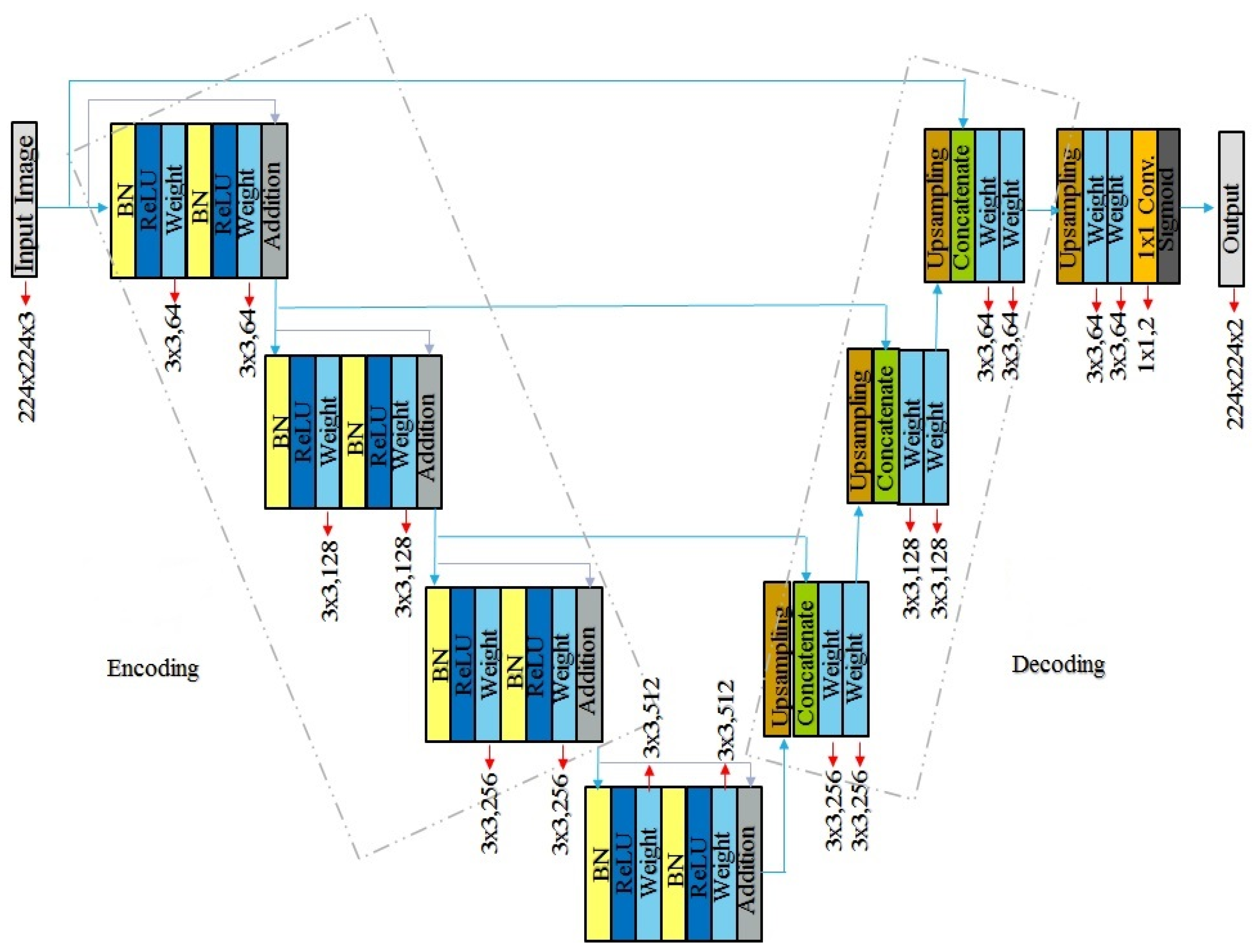
2.1. The Proposed Model

Since the aim of this work is to extract road networks from aerial images, the model must successfully handle semantic segmentation problems. One of the best architectures for such tasks is the U-Net model [31]. The two symmetric parts of the U-net help to extract the road pixels in the encoding part and generate the segmentation map for these pixels in the decoding part. In addition, ResBlocks [26,27] help to ease the training process while being deeper due to all the stacked layers. U-Net also produced better results than regular CNNs in classification and segmentation problems. The proposed model consists of a U-net for the encoding and decoding parts, ResBlocks in the encoding part to enhance the feature extraction process, and Conv. layers in the decoding part to create the segmentation map. The architecture of the proposed model is shown in Figure 1.
Because the input image size of ResNet is 224 × 224 pixels, the ResBlocks in the encoding part of the proposed model will preferably use the same input image size. In the encoding part, three ResBlocks with a filter size of 3 × 3 pixels are implemented, and these three ResBlocks have 64, 128, and 256 filters, respectively. An additional ResBlock with 512 filters connects the encoding and decoding parts. The ResBlocks in the encoding part consist of an activation function (ReLU) after the batch normalization layer (BN), and before the convolution layer (weight) with a shortcut or the identity map (Addition), as described in [26,27]. Each ResBlock in the encoding part is connected with a Conv. layer in the decoding part by a concatenation layer that represents the skip connection for the U-Net [31], and these Conv. layers have 256, 128, and 64 filters, respectively. The proposed model is in auto–encoder pattern, which means that the encoding part is similar to a regular CNN but without the fully connected layers. The output image of the encoding part will be smaller and low resolution than the input image. In the auto-encoder pattern, the decoding part will be implemented instead of the fully connected layers. To increase the size of the image from the encoding part, we need to use an upsampling layer to double the size of the output image in the decoding part, which corresponds to the output of the neural network. Before each concatenation layer in the decoding part, an upsampling layer is implemented to double the size and increase the resolution of the feature map, which had already been downsized in the encoding part. This change will allow the feature map to be used as an input for the segmentation part. The size of the output image will be equal to the input image size (see Figure 1).
It should be noted that the Conv. layers in the decoding part consist of two layers. These layers use the same filter size of 3 × 3 pixels and have 256, 128, and 64 filters, respectively. The second Conv. layer has been added to increase the number of layers and to facilitate the process of upsampling the feature maps. After connecting the encoding and decoding parts together, the process continues in two 64-filter Conv. layers with a filter size of 3 × 3 pixels. The final layer is a 1 × 1 convolutional layer using a sigmoid activation function to produce a binary mask with a size of 224 × 224 pixels as an output. The process is shown in Figure 1.

2.2. Dataset

The dataset used in this work is the high-resolution images set from Cheng et al. [36], who collected the data from Google Earth [37]. Cheng et al. manually labeled the ground truth for each image. The images have a resolution of 1.2 m per pixel, and the dataset consists of 224 differently sized images. The smallest image size is 600 × 600 pixels, and the road width is approximately 12–15 pixels. The images have substantial occlusion from buildings, trees, and cars, which makes the task of extracting road networks from these images difficult.
Before feeding this dataset to the proposed model, it is randomly divided into two sets with 80% of the images assigned to the training set and 20% to the test set.
Since the dataset consists of different image sizes and since 224 images are not enough to train a deep neural network, the images and ground truths that are used in the training and test sets were cropped to 224 × 224 pixels to correspond to the input images’ size; this cropping was done by using a sliding window with a stride of 64 pixels [35,38]. The cropping technique alone increases the number of images in the dataset to 8064 images, where 6480 images are used for the training set and 1584 images were used for the test set. All the cropped images were preprocessed using the on-the-fly data augmentation technique in the Keras framework [39], which helps to increase the number of images within each epoch in the training process. The number of images reached 1,146,938 for the 88th epoch. The standard Keras data augmentations include random rotations, random width and height shifts, shearing, zooming, and horizontal and vertical flips. Data augmentation is the most powerful technique to prevent the overfitting problem.

3. Results

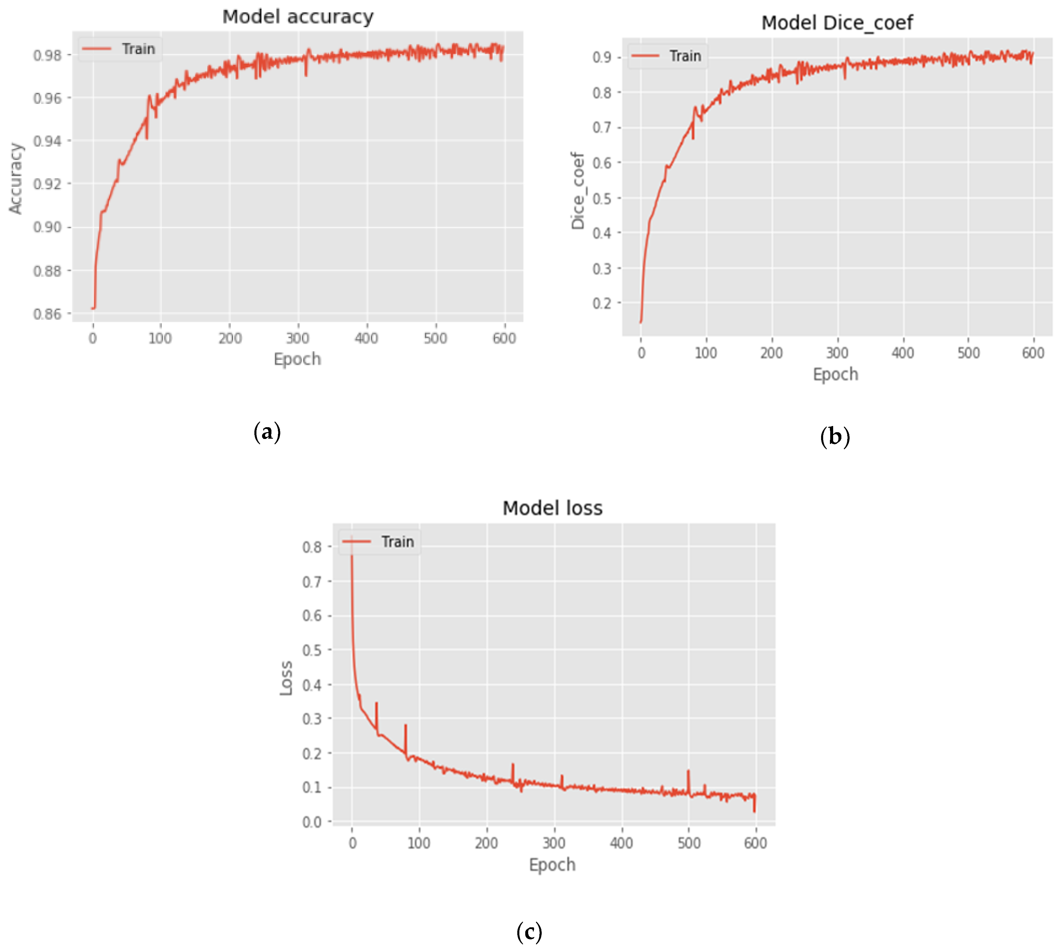
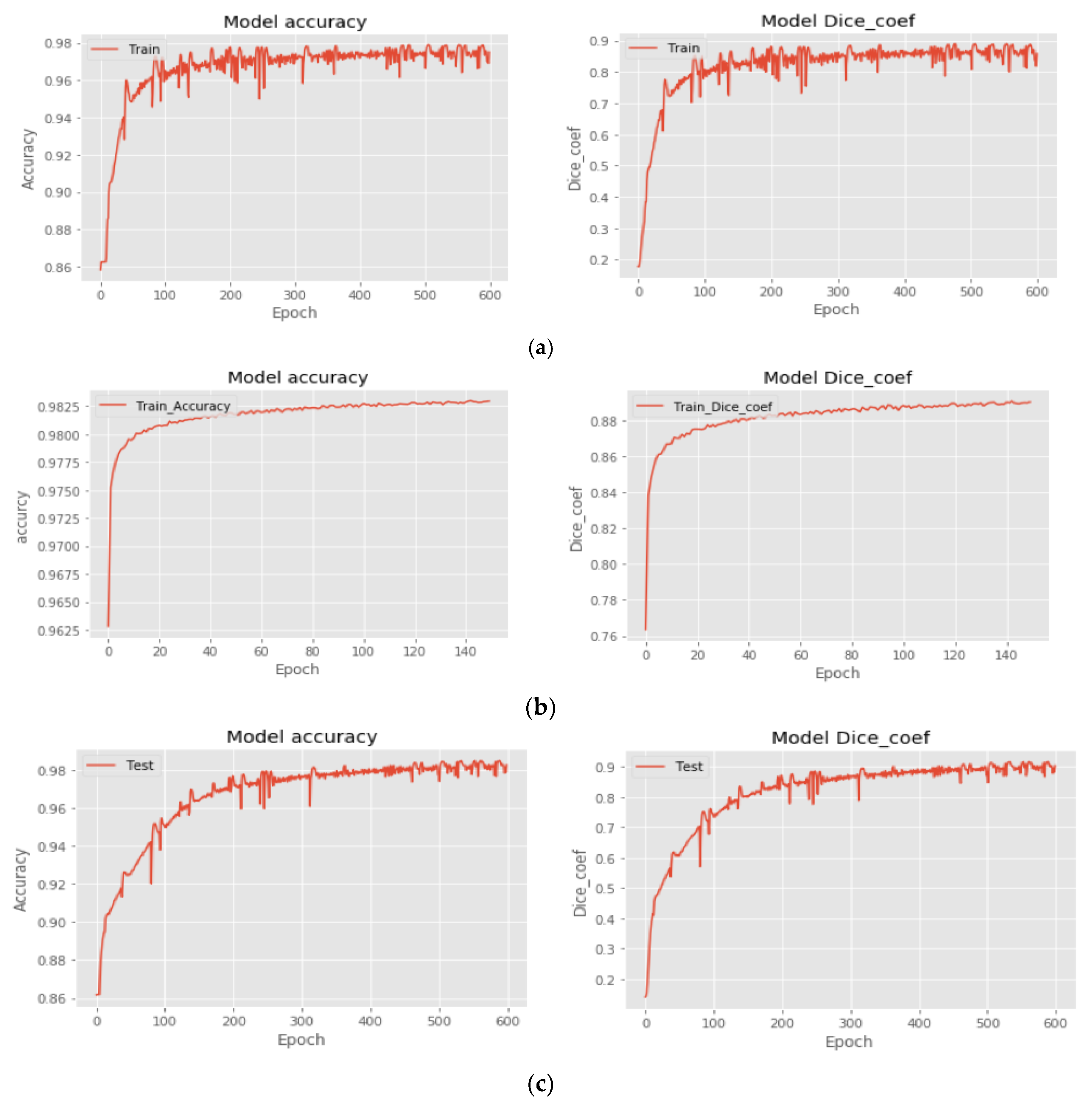
3.1. Training and Implementation Details

The model is implemented using the Keras framework [39] operating on a Microsoft Windows 10 computer with one NVIDIA GeForce GTX 1070 GPU. The optimizer that was used during training is Adam [40], and the learning rate is set at 0.0001. To maximize the model’s efficiency, the loss or error should be minimized. Because the task is binary segmentation, the binary cross-entropy is used as a loss function (Equation(1)): [41,42]
L ( y , p ( y ) ) = 1 N i = 0 n ( y log p ( y ) ) + ( 1 y ) log ( 1 p ( y ) )
where p(y) is the predicted value, y is the true label, and N is the number of samples.
To assess the performance efficiency of the proposed model, two evaluation metrics were used. The first metric is the overall accuracy (OAA), which is defined in Equation (2) [43,44]. The definitions of TP, TN, FP, and FN are shown in Table 1.
O A A = T P + T N T P + T N + F P + F N
The other metric is the Dice similarity coefficient (DSC) [45,46,47,48], which is also known as Czekanowski’s binary index, Zijdenbos’ similarity index, or the F1 score [46]. The DSC is a metric to measure the segmentation performance, and it is shown in Equation (3). If the DSC is equal to 1, the road is perfectly segmented. Conversely, if the DSC is equal to 0, the roads are completely missegmented.
D S C = 2 T P 2 T P + F P + F N
It is preferable to use more than one metric in the evaluation process. The OAA uses the TN, while the DSC does not. The DSC counts the true positives (TPs) twice, and it is more suitable for evaluating the results for imbalanced datasets. It should be mentioned that the authors do not use a pretrained model in the training process, and our model is trained from scratch. The results of the evaluation metrics in Equations (2) and (3) are shown in Table 2 and Figure 2.
The proposed model provides good results according to the evaluation metrics with a 98.35% overall accuracy and a 90.97% DSC.
According to Figure 3(1), the proposed model produces a reasonable prediction that is comparable to the ground truth image. It should be mentioned that the labeling of the ground truth images includes two problems: the shoulders of the roads in the true labels are sometimes marked as part of the road and sometimes they are not (Figure 3(2)–(4)), and some side roads or local roads are incorrectly labeled in the ground truth image (Figure 3(5)). The first problem increases the difficulties of extracting clear edges for the road networks, but our model produced correct predictions in most of the images, as shown in Figure 3(2)–(4). The proposed model overcame the second problem, as shown in Figure 3(5).
With respect to the problems of the labels that were mentioned above, it is very difficult to observe these problems, even after cropping the images into small sizes, and subsequently, it is very difficult to correct them. These problems are very common when labeling datasets because these labels are manually set, and they are prone to human errors.

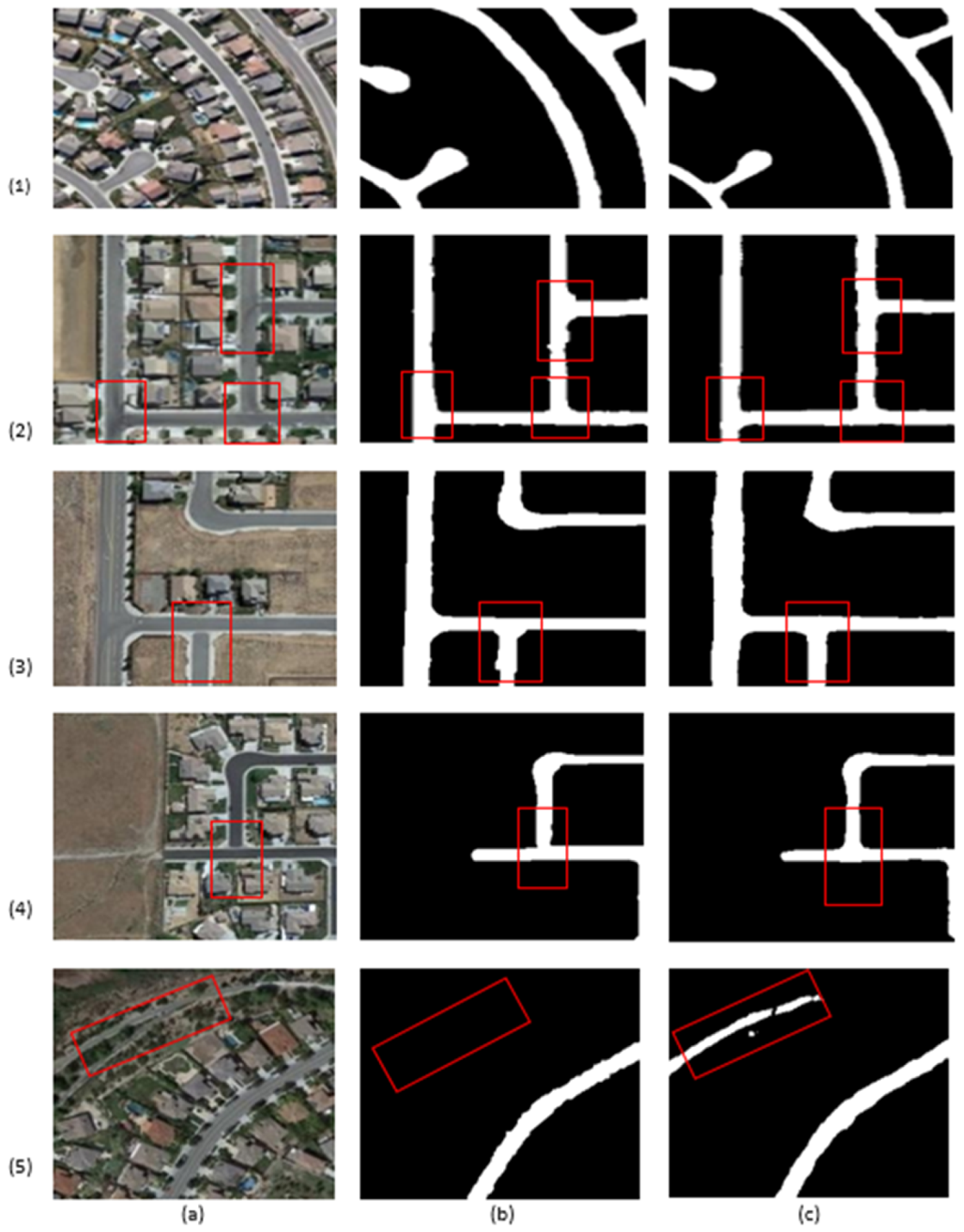
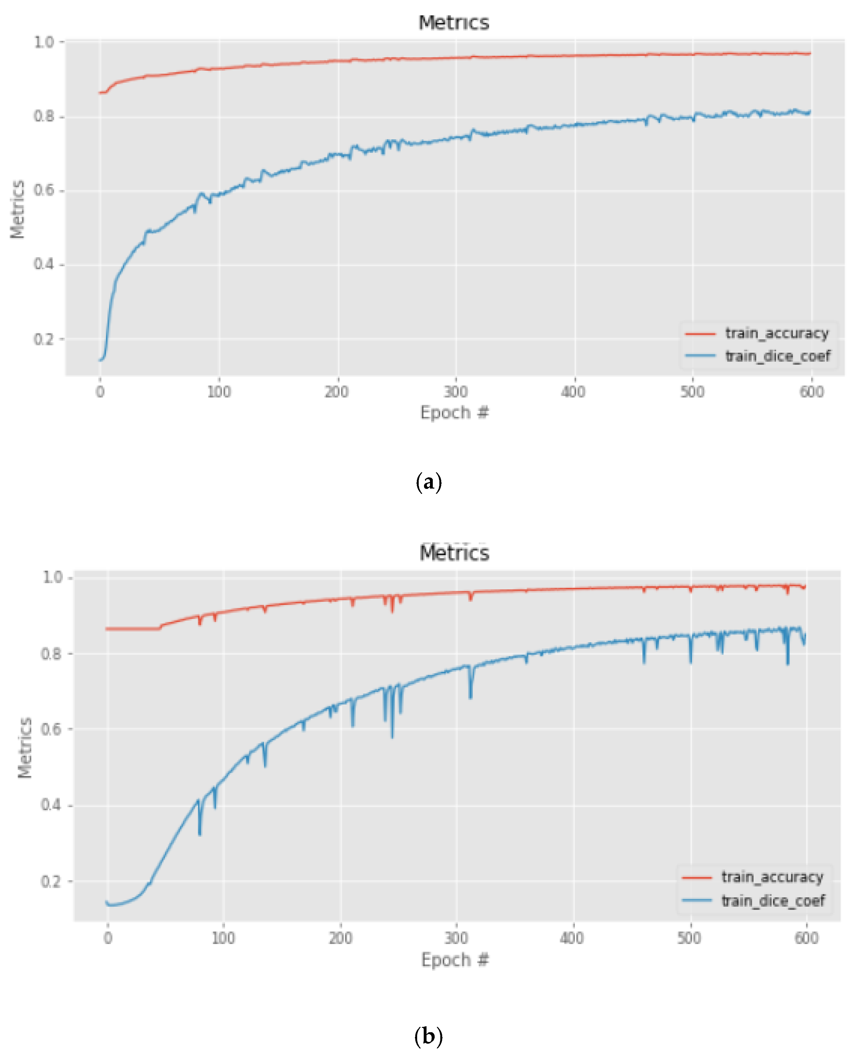
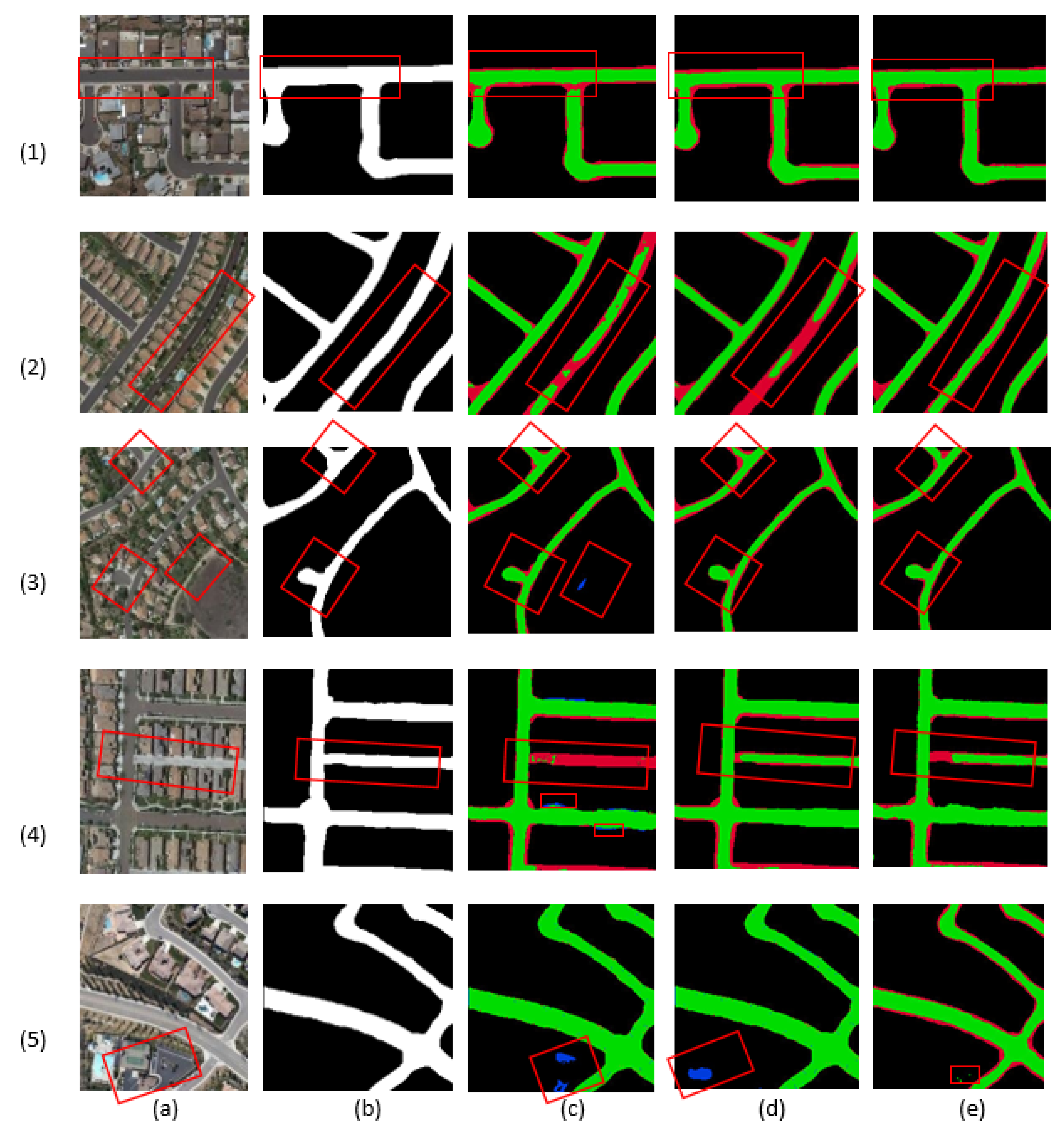
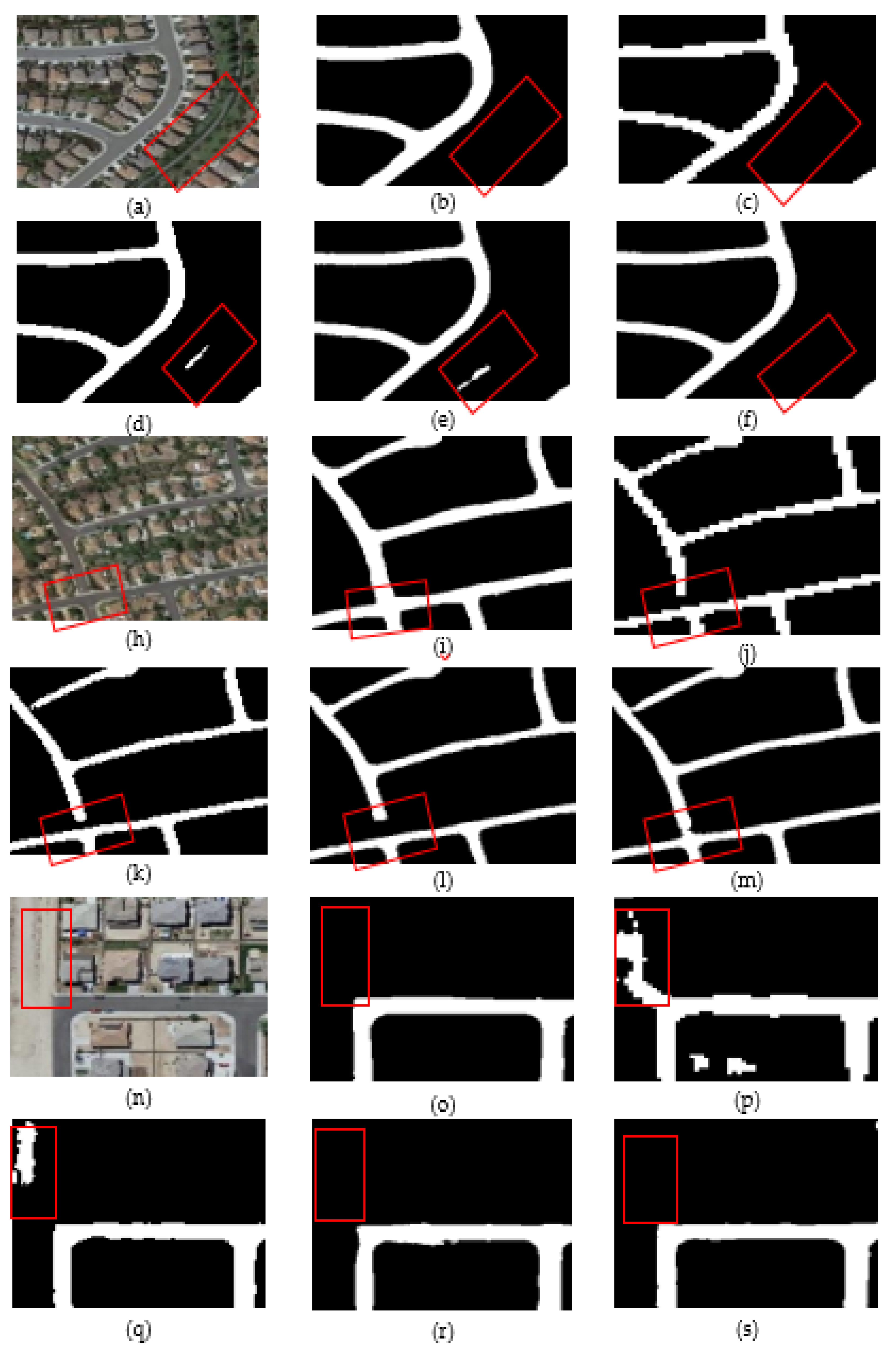
3.2. Comparisons with Other models

To evaluate the validity of our model, these results were compared with those of other state-of-the-art models. For the sake of clarity, it should be mentioned that the authors trained these models in the same manner as described in Section 3.1.
To make a meaningful comparison, the models that were considered were models that generally produced good results in semantic segmentation tasks. Because the proposed model is a combination of U-Net [31] and ResBlocks [26,27], it was most suitable to compare the proposed model with Res-Unet [33] and U-net [31]. Table 3 and Figure 4 show the evaluation metrics (OAA and DSC) for the U-Net and Res-Unet models and for the proposed model.
The proposed model achieved a better OAA and DSC than the Res-Unet and U-net models. Figure 5 presents a more detailed explanation and analyses. It shows the differences among the predictions that were made by Res-Unet, U-Net, and the proposed models. Figure 5(1) shows good predictions for the intersecting roads for U-Net and the proposed model, while the Res-Unet model was less successful in this task. Figure 5(2) shows that the proposed model performed significantly better than both the U-Net and Res-Unet models in predicting different types of roads, which had different pavement colors in the original image. In Figure 5(3), Res-Unet mistakenly recognized background pixels as the road class, while U-Net and the proposed model predicted them correctly. For intersecting roads, the three models performed similarly in making predictions.
Figure 5(4), which captured local roads, shows the predictions of different types of roads that had different pavement colors in the original image. The U-net model provides better results than the proposed model, and the Res-Unet model failed to make a correct prediction.
Figure 5(5) shows a case in which our model clearly outperformed both Res-Unet and Unet. While these two models predicted different parts of parking lot pixels as road pixels, our model predicted almost all these pixels as the background class.
The evaluation metrics that are shown in Table 3 and Figure 4 combined with The results that are shown in Figure 5, suggest that the proposed model produces generally better results over both Res-Unet and U-Net for extracting road networks.

4. Discussion

U-Net has provided remarkable results in semantic segmentation tasks, and it has been combined with other architectures in many studies [33,34,35,36,37,38]. ResNet and ResBlocks [26,27] have also been shown to well enhance the design of deep neural networks in general, to ease training while stacking more layers in the network and to overcome the vanishing gradient problem. Numerous designs had been tested to choose the optimal design that provides the most accurate segmentation results compared to our model.
Our first trial method was an auto-encoder design with ResBlocks [26,27] in both the encoding and decoding parts. The ResBlocks [26,27] have a similar architecture to the ResNet-18 layers in an auto-encoder structure. We trained and evaluated the model, The evaluation metrics show an OAA of 97.51% and a DSC of 85.84% (Table 4 and Figure 6), and the predictions that are shown in Figure 7c,j,p have several issues: unclear edges for the extracted roads, prediction problems in some intersecting roads, and background pixels mistakenly predicted as the road class.
Based on the analysis mentioned above that was related to the first model, when designing our second model, we enhanced it by adding a long skip connection for U-net [31] to avoid the unsatisfactory results of the first model. In addition, an extra ResBlock with 1024 filters was included as a bridge or connection between the encoding and decoding parts. Figure 7d,k,q show that better predictions were achieved in the second trial compared with the first. The edges that were extracted for the roads have been enhanced, and the two issues related to mistakenly predicted pixels and the detection of intersecting roads were somewhat improved. The second model has an OAA of 98.30% and a DSC of 89.02% (Table 4 and Figure 6).
The third model was similar to the proposed model, but the ResBlocks were designed following the original model that was described by He et al. [24]. In Figure 7e,l,r, we can see that the predictions that it produced were similar to (e,l) or slightly improved upon (r) the second model. The results show an OAA of 98.33% and DSC of 89.23% (Table 4 and Figure 6).
After analyzing all the predictions from the three models that were mentioned above, the final model that was used was the proposed one, as shown in Figure 1. Figure 7 compares the predictions of the proposed model with those of the previous models. The OAA and DSC of the proposed model were 98.35% and 90.79%, respectively (Table 4 and Figure 6). The proposed model achieved the best prediction and results for the road extraction task in comparison with earlier models. The evolution of these models clarifies the importance of the combination of the skip connection for U-Net [29], the ResBlocks [24,25], and the plain convolutional layers. The combination provides a simple shape yet an effective architecture. Although the proposed model is simple, it helps to efficiently and accurately extract the road networks, and it achieved the goal of this paper.
The current results of our study are the first step to continuing our work to develop a real-time road extraction algorithm that can be embedded in any machine. The second step will be extracting the centerline of the road. In combination with the result of the first step for the road extraction, this algorithm will help to estimate the approximate width of the road and the type of the road. This step has huge importance in city planning, the geometric design of highways, transportation engineering, traffic engineering, and disaster mitigation. To achieve that goal, several steps will be included in the future work, including creating our own dataset focused on road and centerline extraction, using the weight of the proposed model to train the new data to improve the prediction performance when utilizing the transfer learning technique, and working to achieve the goal of obtaining a real-time road extraction model that can be used as embedded software.

5. Conclusions

In this paper, a new Res-Unet has been presented. The proposed architecture is a simpler, lighter, and simultaneously more efficient segmentation model. Many earlier experiments were conducted using different algorithms, and these experiments showed that the combination of the U-net, ResBlocks, and plain convolutional layers gave the best results in comparison with other state-of-the-art models. This study represents our first step toward achieving our goal of creating a real time road extraction model that can be used in any machine. The study also lists several steps that can be used in our future work. For example, the performed experiments and the comparison of predictions with the ground truth images revealed the importance of the availability of good, correctly labeled ground truth images and their impact on the predicted results. This finding should be considered when creating our two datasets for road extraction and centerline extraction. It is expected that the proposed model will give better results when using the pretrained model, and this hypothesis will be tested in future work. In these future studies, we will use transfer learning to train the proposed model on our new dataset.

Author Contributions

T.A. conceived the work, processed the data, and wrote the paper. W.L. and Y.M. supervised the data processing and revised the manuscript.

Funding

This research receives no external funding.

Conflicts of Interest

The authors declare no conflict of interest.

References

  1. Wang, W.; Yang, N.; Zhang, Y.; Wang, F.; Cao, T.; Eklund, P. A review of road extraction from remote sensing images. J. Traffic Transp. Eng. (Engl. Ed.) 2016, 3, 271–282. [Google Scholar] [CrossRef]
  2. Bacher, U.; Mayer, H. Automatic road extraction from multispectral high resolution satellite images. In Proceedings of the ISPRS Workshop CMRT 2005: Object Extraction for 3D City Models, Road Databases and Traffic Monitoring - Concepts, Algorithms and Evaluation Vienna, Austria, 29–30 August 2005; ISPRS Archives: Vienna, Austria, 2005; Volume XXXVI-3/W24, p. 6. [Google Scholar]
  3. Bicego, M.; Dalfini, S.; Vernazza, G.; Murino, V. Automatic Road Extraction from Aerial Images by Probabilistic Contour Tracking. In Proceedings of the 2003 International Conference on Image Processing (Cat. No. 03CH37429), Barcelona, Spain, 14–17 September 2003; Volume 3, p. 585. [Google Scholar] [CrossRef]
  4. Wei, Y.; Wang, Z.; Xu, M. Road structure refined CNN for road extraction in aerial images. IEEE Geosci. Remote Sens. Lett. 2017, 14, 709–713. [Google Scholar] [CrossRef]
  5. Amo, M.; Martinez, F.; Torre, M. Road extraction from aerial images using region competition algorithm. IEEE Trans. Image Process. 2006, 15, 1192–1201. [Google Scholar] [CrossRef] [PubMed]
  6. Heipke, C.; Mayer, H.; Wiedemann, C. Evaluation of automatic road extraction. Int. Arch. ISPRS J. Photogramm. Remote Sens. 1997, 32, 47–56. [Google Scholar]
  7. Gamba, P.; DellAcqua, F.; Lisini, G. Improving urban road extraction in high-resolution images exploiting directional filtering, perceptual grouping, and simple topological concepts. IEEE Geosci. Remote Sens. Lett. 2006, 3, 387–391. [Google Scholar] [CrossRef]
  8. Gruen, A.; Li, H. Road extraction from aerial and satellite images by dynamic programming. ISPRS J. Photogramm. Remote Sens. 1995, 50, 11–20. [Google Scholar] [CrossRef]
  9. Heipke, C.; Steger, T.; Multhammer, R. Hierarchical approach to automatic road extraction from aerial imagery. In Proceedings of the SPIE 2486, Integrating Photogrammetric Techniques with Scene Analysis and Machine Vision II, Orlando, FL, USA, 5 July 1995; p. 2486. [Google Scholar] [CrossRef]
  10. Long, H.; Zhao, Z. Urban road extraction from high-resolution optical satellite images. Int. J. Remote Sens. 2005, 26, 4907–4921. [Google Scholar] [CrossRef]
  11. Hormese, J.; Saravanan, C. Automated road extraction from high resolution satellite images. Procedia Technol. 2016, 24, 1460–1467. [Google Scholar] [CrossRef]
  12. Li, Y.; Briggs, R. Automatic extraction of roads from high resolution aerial and satellite images with heavy noise. Int. J. Comp. Inf. Eng. 2009, 3, 1571–1577. [Google Scholar] [CrossRef]
  13. Hu, X.; Zhang, Z.; Zhang, J. An approach of semiautomated road extraction from aerial image based on template matching and neural network. Int. Arch. ISPRS J. Photogramm. Remote Sens. 2000, 33, 994–999. [Google Scholar]
  14. Xia, W.; Zhang, Y.; Liu, J.; Luo, L.; Yang, K. Road extraction from high resolution image with deep convolution network—A case study of GF-2 image. In Proceedings of the 2nd International Electronic Conference on Remote Sensing (ECRS 2018), 22 March–5 April 2018; Volume 2, p. 325. Available online: www.sciforum.net/conference/ecrs-2 (accessed on 20 May 2019). [CrossRef]
  15. Kahraman, I.; karas, I.R.; Akay, A.E. Road extraction techniques from remote sensing images: A review. In The International Archives of the Photogrammetry, Remote Sensing and Spatial Information Sciences, Proceedings of the International Conference on Geomatics and Geospatial Technology (GGT 2018), Kuala Lumpur, Malaysia, 3–5 September 2018; XLII-4/W9; pp. 339–342. [CrossRef]
  16. Shackelford, A.; Davis, C. Fully automated road network extraction from high-resolution satellite multispectral imagery. In Proceedings of the IGARSS 2003, 2003 IEEE International Geoscience and Remote Sensing Symposium (IEEE Cat. No.03CH37477), Toulouse, France, 21–25 July 2003; Volume 1, pp. 461–463. [Google Scholar] [CrossRef]
  17. Hu, X.; Vincent Tao, C.; Hu, Y. Automatic road extraction from dense urban area by integrated processing of high imagery and LIDAR data, processing of high resolution imagery and LIDAR data. In Proceedings of the International Archives of Photogrammetry, Remote Sensing and Spatial Information Sciences IAPRSIS, Istanbul, Turkey, –23 July 2004; Volume 35, pp. 288–292. [Google Scholar]
  18. Saito, S.; Yamashita, T.; Aoki, Y. Multiple object extraction from aerial imagery with convolutional neural networks. J. Imaging Sci. Tech. 2016, 60, 10402-1–10402-9. [Google Scholar] [CrossRef]
  19. Vosselman, G.; De Knecht, J. Road Tracing by Profile Matching and Kalman filtering, Workshop on Automatic Extraction of Manmade Objects from Aerial and Space Images; Birkhauser: Berlin, Germany, 1995; pp. 265–274. [Google Scholar] [CrossRef]
  20. Mokhtarzade, M.; Valadan Zoej, M. Road detection from high- resolution satellite images using artificial neural networks, inter. J. Appl. Earth Obs. Geoinf. 2007, 9, 32–40. [Google Scholar] [CrossRef]
  21. Krizhevsky, A.; Hinton, G. Image net classification with deep convolutional neural networks. In Proceedings of the 25th International Conference on Neural Information Processing Systems, Lake Tahoe, NV, USA, 3–6 December 2012; Volume 1, pp. 1097–1105. [Google Scholar]
  22. Mnih, V.; Hinton, G. Learning to detect roads in high-resolution aerial images. In Proceedings of the 11th European Conference on Computer Vision ECCV’10, Crete, Greece, 5–11 Spetember 2010; Part VI. pp. 210–223. [Google Scholar] [CrossRef]
  23. Vicini, D.; Hamas, M.; Taivo, P. Road Extraction from Aerial Images. Available online: https://github.com/mato93/road-extraction-from-aerial-images (accessed on 15 June 2019).
  24. Wang, S.; Sun, J.; Phillips, P.; Zhao, G.; Zhang, Y. Polarimetric synthetic aperture radar image segmentation by convolutional neural network using graphical processing units. J. Real Time Image Process. 2017, 15, 631–642. [Google Scholar] [CrossRef]
  25. Li, Z.; Wang, S.; Fan, R.; Cao, G.; Zhang, Y.; Guo, T. Teeth category classification via seven-layer deep convolutional neural network with max pooling and global average pooling. Int. J. Image Syst. Technol. IMA 2019. [Google Scholar] [CrossRef]
  26. Kaiming, H.; Zhang, X.; Ren, S.; Sun, J. Deep residual learning for image recognition. In Proceedings of the 2016 IEEE Conference on Computer Vision and Pattern Recognition (CVPR), Las Vegas, NV, USA, 27–30 June 2015; pp. 770–778. [Google Scholar] [CrossRef]
  27. Kaiming, H.; Zhang, X.; Ren, S.; Sun, J. Identity mappings in deep residual networks. In Proceedings of the 14th European Conference on Computer Vision, Amsterdam, The Netherlands, 8–16 October 2016; Part IV. pp. 630–645. [Google Scholar] [CrossRef]
  28. Long, J.; Shelhamer, E.; Darrell, T. Fully convolutional networks for semantic segmentation. In Proceedings of the 2015 IEEE Conference on Computer Vision and Pattern Recognition (CVPR), Boston, MA, USA, 7–12 June 2015; pp. 3431–3440. [Google Scholar] [CrossRef]
  29. Simonyan, K.; Zisserman, A. Very deep convolutional networks for large-scale image recognition. Proceeding of International Conference on Learning Representations ICLR, San Diego, CA, USA, 7–9 May 2015. [Google Scholar]
  30. Szegedy, C.; Liu, W.; Jia, Y.; Sermanet, P. Going deeper with convolution. In Proceedings of the IEEE Conference on Computer Vision and Pattern Recognition (CVPR), Boston, MA, USA, 7–12 June 2015; pp. 1–9. [Google Scholar] [CrossRef]
  31. Ronneberger, O.; Fischer, P.; Brox, T.; U-Net. Convolutional networks for biomedical image segmentation. In Medical Image Computing and Computer-Assisted Intervention—MICCAI 2015, Proceeding of 18th International Conference, Munich, Germany, 5–9 October 2015; Springer International Publishing: Cham, Swizerland, 2015; Volume 9351, pp. 234–241. [Google Scholar] [CrossRef]
  32. Badrinarayanan, V.; Kendall, A. SegNet: A deep convolutional encoder-decoder architecture for image segmentation. IEEE Trans. Pattern Anal. Mach. Intell. 2017, 39, 2481–2495. [Google Scholar] [CrossRef] [PubMed]
  33. Zhang, Z.; Liu, Q.; Wang, Y. Road extraction by deep residual U-Net. IEEE Geosci. Remote Sensing Lett. 2018, 15, 749–753. [Google Scholar] [CrossRef]
  34. Buslaev, A.; Seferbekov, S.S.; Iglovikov, V.I.; Shvets, A.A. Fully convolutional network for automatic road extraction from satellite imagery. In Proceedings of the IEEE/CVF Conference on Computer Vision and Pattern Recognition Workshops (CVPRW), Salt Lake City, UT, USA, 18–22 June 2018; pp. 197–1973. [Google Scholar] [CrossRef]
  35. Xu, Y.; Xie, Z.; Feng, Y.; Chen, Z. Road extraction from high-resolution remote sensing imagery using deep learning. Remote Sens. 2018, 10, 1461. [Google Scholar] [CrossRef]
  36. Cheng, G.; Wang, Y.; Xu, S.; Wang, H.; Xiang, S.; Pan, C. Automatic road detection and centerline extraction via cascaded end-to-end convolutional neural network. IEEE Trans. Geosci. Remote Sens. 2017, 55, 3322–3337. [Google Scholar] [CrossRef]
  37. Google. Google Earth. Available online: http://www.google.cn/intl/zh-CN/earth/ (accessed on 20 May 2019).
  38. Wang, H.; Wnag, Y.; Zhang, Q.; Xinag, S.; Pan, C. Gated convolutional neural network for semantic segmentation in high-resolution images. Remote Sens. 2017, 9, 446. [Google Scholar] [CrossRef]
  39. Keras. 2015. Available online: https://github.com/fchollet/keras (accessed on 8 November 2019).
  40. Kingma, D.P.; Ba, J. ADAM: A method for stochastic optimization. In Proceedings of the 3rd International Conference on Learning Representations, San Diego, CA, USA, 7–9 May 2015. [Google Scholar]
  41. Binarycrossentropy. Available online: https://peltarion.com/knowledgecenter/documentation/modeling-view/build-an-ai-model/loss-functions/binary-crossentropy (accessed on 9 April 2019).
  42. Understanding Binary Cross-Entropy/Log Loss: A Visual Explanation. Available online: https://towardsdatascience.com/understanding-binary-cross-entropy-log-loss-a-visual-explanation-a3ac6025181a (accessed on 9 April 2019).
  43. Powers, D. What the F-measure doesn’t measure: Features, flaws, fallacies and fixes. arXiv 2015, arXiv:1503.06410. [Google Scholar]
  44. Taylor, J.R. An Introduction to Error Analysis: The Study of Uncertainties in Physical Measurements, 2nd ed.; University Sciences Books: Sausalito, CA, USA, 1999; pp. 128–129. [Google Scholar]
  45. Zou, K.H.; Warfield, S.K. Statistical validation of image segmentation quality based on a spatial overlap index: Scientific Reports. Acad. Radiol. 2004, 11, 178–189. [Google Scholar] [CrossRef] [Green Version]
  46. Al-Faris, A.Q.; Ngah, U.K.; Isa, N.; Shuaib, I.L. MRI breast skin-line segmentation and removal using integration method of level set active contour and morphological thinning algorithms. J. Med. Sci. 2012, 12, 286–291. [Google Scholar] [CrossRef] [Green Version]
  47. Cardenes, R.; Luis-Garcia, R.; Bach-Cuadra, M. A multidimensional segmentation evaluation for medical image data. Comput. Methods Prog. Biomed. 2009, 96, 108–124. [Google Scholar] [CrossRef] [PubMed]
  48. Derczynski, L. Complementarity F-score and NLP Evaluation. In Proceedings of the 10th Edition of the Language Resources and Evaluation Conference, Portoroz, Slovenia, 23–28 May 2016. [Google Scholar]
Figure 1. Proposed model.
Applsci 09 04825 g001
Figure 2. Evaluation of the proposed model in terms of (a) the overall accuracy, (b) the DSC, and (c) the loss.
Applsci 09 04825 g002
Figure 3. Comparisons of (a) the original images, (b) the ground truth images, and (c) the predictions of the proposed model.
Applsci 09 04825 g003
Figure 4. Comparisons of the OAAs and DSCs for (a) the Res-Unet and (b) the U-Net.
Applsci 09 04825 g004
Figure 5. Comparisons among (a) the original images, (b) the ground truth images, (c) the predictions of Res-Unet, (d) the predictions of U-Net, and (e) the predictions of the proposed model. Green, red and blue represent TPs, FPs and FNs, respectively.
Applsci 09 04825 g005
Figure 6. Comparisons of the OAAs and DSCs for (a) the Auto-encoder.ResNet, (b) the Full Res-Unet, and (c) the Res-Unet (Orig. Rse.).
Applsci 09 04825 g006
Figure 7. Comparison of the results between the proposed model and different models: (a,h,n) the original images, (b,i,o) the ground truth images, (c,j,p) the predictions of the first model, (d,k,q) the predictions of the second model,(e,l,r) the predictions of the third model, and (f,m,s) the predictions of the proposed model.
Applsci 09 04825 g007
Table 1. Definitions of TP, TN, FP, and FN
Predicted
Road
(1)
Background
(0)
ActualRoad
(1)
True positive (TP)False positive (FP)
Background
(0)
False negative (FN)True negative (TN)
Table 2. The results of the evaluation metrics
OAADSC
Proposed Model98.35%90.97%
Table 3. The comparison results.
ModelOAADSC
Res-Unet96.96%81.73%
U-Net97.52%84.84%
Our Model98.35%90.97%
Table 4. Comparison of the results.
ModelOverall AccuracyDSC
Auto-encoder.ResNet (first trial)97.51%85.84%
1Full Res-Unet
(second model)
98.30%89.02%
Res-Unet (2Orig. Rse.)
(third model)
98.33%89.23%
Our Model98.35%90.97%
1 Full Res-Unet where ResBlocks are used in both the encoding and decoding parts, 2 Orig. Rse. is the Original ResBlock.

