1. Introduction
Market success of a manufacturing company is shaped primarily by the demand for the manufactured products and the rate of return on capital employed [
1,
2]. Poor machine efficiency and frequent downtimes can lead to a reduction in production levels, resulting in lost market opportunities, increased operating costs and reduced profits [
3]. It is therefore necessary to apply appropriate methods and tools to support management and to organize maintenance services in an adequate manner to ensure that the production system operates at the assumed levels of productivity and efficiency [
4].
Effectiveness is an important element in the analysis of the production process [
5,
6,
7], often considered in scientific publications. It is assessed on the basis of various measures. In practice, numerous mathematical models and tools are used to support the assessment of the performance of machinery. The most frequently used measures for analyzing the efficiency of technical facilities are those resulting from three general models of operation assessment, i.e., the reliability model, the operational efficiency OEE (overall equipment effectiveness) model and the organizational and technical KPI (key performance indicators) model [
8]. In addition, methods and tools for its evaluation can be classified in five main areas, i.e., operational, market, financial, technical or dynamic [
9,
10]. Particularly important from the point of view of machinery efficiency diagnostics is operational efficiency, and the research in this area focuses primarily on the search for opportunities to reduce the consumption of production resources. These include analysis of labor productivity growth, cost reduction, minimization of losses and shortening of production cycles. Studies available in the literature indicate the application of a number of methods and tools in this area, such as methods of productivity and profitability indicators, analysis of efficiency and degree of work stations’ utilization, cost calculation of activities, study of spatial efficiency of production organization and economic evaluation of the production structure [
11].
Maintaining the company’s machinery stock at an appropriate level requires continuous monitoring and evaluation of the adopted effectiveness indicators. A number of companies have MES (manufacturing execution system) systems in place, which enable ongoing control of the above parameters. There are also companies (including those examined by the authors) that do not have such software and therefore proper evaluation of efficiency parameters is difficult. Such analyses are supported by mathematical tools and methods, which also include modeling with the use of logistic regression, as presented in this article. The subject of this research was a plastics manufacturing company, while the main objective was to evaluate the effectiveness of the production process based on selected factors that may significantly affect the level of machinery efficiency. The analysis was carried out on the basis of information on the performance of the company’s production system recorded from 1 September 2015 to 31 August 2017.
Monitoring the effectiveness of utilization of the available machinery allows production reserves or waste in the processes underway to be identified [
12,
13,
14]. The basis for successful assessment is an appropriate selection of measures and indicators. The analysis of literature made it possible to distinguish those which were of the greatest importance both in theoretical and industrial-practical aspects. Three general models should be distinguished:
Within the operational efficiency model, a frequently employed parameter (which was monitored in the examined entity as well) is the overall equipment effectiveness (OEE) indicator, which is widely described in the literature [
16,
17,
18,
19]. The available studies most often present the theoretical aspects of its calculation and indicate the categories of losses that may occur during the process of machinery and equipment use in relation to ideal conditions [
19,
20,
21]. Analyses are also available to demonstrate the practical implementation of this parameter in manufacturing companies [
12,
22,
23].
The OEE index is a product of three components [
23,
24], i.e., readiness and efficiency of machinery and quality of the manufactured products. It is therefore a general, comprehensive assessment, most often presented in percentage form. According to Seichi Nakajime from the Japan Institute of Plant Maintenance [
25,
26], OEE should remain at 85.41%, but it should be stressed that each enterprise operates in a specific environment; thus, this indicator will be different for each entity, depending on its size, profile and industry, and will not take on the same value in two different operating units [
9,
27]. Therefore, in practice the above indicator has evolved into different forms of application depending on the sector in which a given entity operates, adjusting to the needs of the environment. The following indicators should be mentioned: OFE (overall factory effectiveness), OPE (overall plant effectiveness), OTE (overall throughput effectiveness), PEE (production equipment effectiveness), OAE (overall asset effectiveness) or TEEP (total equipment effectiveness performance) [
21].
The reliability model allows measures in statistical terms to be determined, on the basis of a time analysis of the performance of technical facilities. In practice, these refer to the technical condition of machines, as well as to the activities of maintenance staff. These are MTBF (mean time between failures), MTTR (mean time to repair) or MTTF (mean time to failure) [
15].
The organizational and technical KPI model includes a set of measures enabling a comprehensive assessment of the efficiency and effectiveness of the implemented processes. It includes 72 indicators classified in three areas: economic (e.g., total relative cost of maintenance), technical (availability of facilities for preventive works) and organizational (number of maintenance staff) [
28].
In relation to the analyzed company, indicators associated with the operational effectiveness model, related to efficiency, will be preferable in the context of machinery stock management; therefore, they have become the subject of this analysis. Following the literature in this field [
13,
29], it was assumed that efficiency in production processes is the quotient of the actual efficiency to the nominal efficiency, as specified in the following ratio (1):
where:
WQ—machinery operational efficiency indicator,
Qr—actual (achieved) efficiency (pcs./h),
QO—theoretical efficiency, as defined in the technical documentation (pcs./h).
Thus calculated, it indicates the degree of efficient use of the production line for each operation and, as such, indicates areas for improvement. Efficiency is most often presented in percentage form. This does not always allow for its quick and unambiguous assessment. In forecasting studies, it is assumed to be a quantitative variable, which limits the availability of some modeling methods. Therefore, with regard to the analyzed company, according to the authors, a better approach would be to analyze the efficiency from the individual point of view of each company by determining its satisfactory level and reacting only if it is not achieved.
Numerous studies using logistic regression models with regard to machine maintenance are available in the literature. The main objective of the proposed tools is to assess the technical condition of technical objects along with reliability parameters [
30,
31], predict upcoming failures [
32,
33] and estimate the service life of machinery [
34]. For example, Yan and Lee assessed the performance of an elevator door system in real time and identified the types of possible failures [
30]. Kozłowski et al. developed a model classifying the condition of a cutting tool blade and predicting its durability [
31]. Lee et al. studied the reliability of a cutting tool using a combination of logistic regression and acoustic emission methods [
32]. Caesarendra combined methods of logistic regression and relevance vector machine to evaluate performance degradation and to predict failure times based on simulation and experimental data [
33], whereas Chen et al., on the basis of vibration characteristics of cutting tools, developed a universal model enabling the analysis of reliability and performance for machine tools [
34].
This article proposes a model of logistic regression to be used for analysis and evaluation of the level of efficiency of executed processes. The research covered the process of manufacturing garbage bags in a company operating several production plants located in Poland and Ukraine. It was carried out in three main stages, in line with the CBM (condition-based maintenance) strategy. The basis for the research were the work and inspection cards of roll making machines provided by the company, which came from one of the plants and covered the period from 1 September 2015 to 31 August 2017. These provided information in two main categories. Event data indicated what events occurred during the operation of the machine (i.e., the need to repair, replacement of worn parts or breakdowns). On the other hand, the condition monitoring data provided information about the current technical condition of the facilities and the need for preventive measures (e.g., adjustment of Teflon blades). The processing of the above information and interpretation thereof made it possible to identify factors shaping the efficiency of the machinery stock. Then, on their basis, a model for the evaluation of machinery efficiency was built. It was assumed that its satisfactory level was 90%. This value is based on the daily production cycle, which also includes the breaks required by the Labor Code, daily service and the preparation of the machine for operation. Finally, the manner in which the model can support decision making in the area of improvement of the production processes was indicated [
35].
Due to the specificity of manufactured products, i.e., serial products with standard parameters, the company operates in the MTS (make to stock) production system. The plant works on a three-shift basis, with each shift lasting 8 h. The process of model parameter estimation and the results obtained are presented in subsequent sections of this article.
2. Logistic Regression Model
Logistic regression is a model that allows the influence of several variables
X1,
X2, …,
Xk on the dichotomous variable
Y in the mathematical form to be presented. The logistic regression model is based on a logistical function that takes the following form:
where
e is the Euler number, and
x is the value of the explanatory variable
X.
The use of logistic regression is supported by the fact that it is not required to meet many assumptions that are formulated in relation to linear regression and general linear models. These include, first of all, the linearity of the relationship between a dependent and an independent variable, as well as the normality and homoscedasticity of the distribution of independent variables. In addition, observations must be reported using metric measurement systems.
The logistic regression model can be written in several ways. Assuming that
Y stands for a dichotomous variable with values 1, for the occurrence of the event we are interested in (success), and 0, for the opposite case (failure), the logistic regression model is described by Equation (3):
where
βi i = 0, …,
k are logistic regression factors, while
x1,
x2, …,
xk are independent variables, which can be measurable or qualitative.
An equivalent form of the logistic regression equation can be written as the odds for the occurrence of the event (success) we are interested in:
In a special case, for one independent variable the logistic regression equation takes the following form:
If, in turn, both sides of the Equation (5) are logarithmized, the logit form of the logistic model will be obtained:
The condition necessary for logistic regression is a sufficiently large sample, the number of which should be , where k is the number of parameters.
Important concepts related to logistic regression are the odds and the odds ratio. The odds are defined as the probability of an event occurring
P(
A) divided by the probability of an event not occurring, 1 −
P(
A):
The odds ratio, in turn, marked
OR, is defined as the odds of one event occurring
S(
A) divided by the odds of another event occurring
S(
B):
3. Estimation of Markov Logistic Model Parameters
The first stage of the study was to define possible explanatory variables in order to determine which of them could be used in the model. The following explanatory variables were selected: shift, device, occurrence of failure (yes or no) and no production order (yes or no).
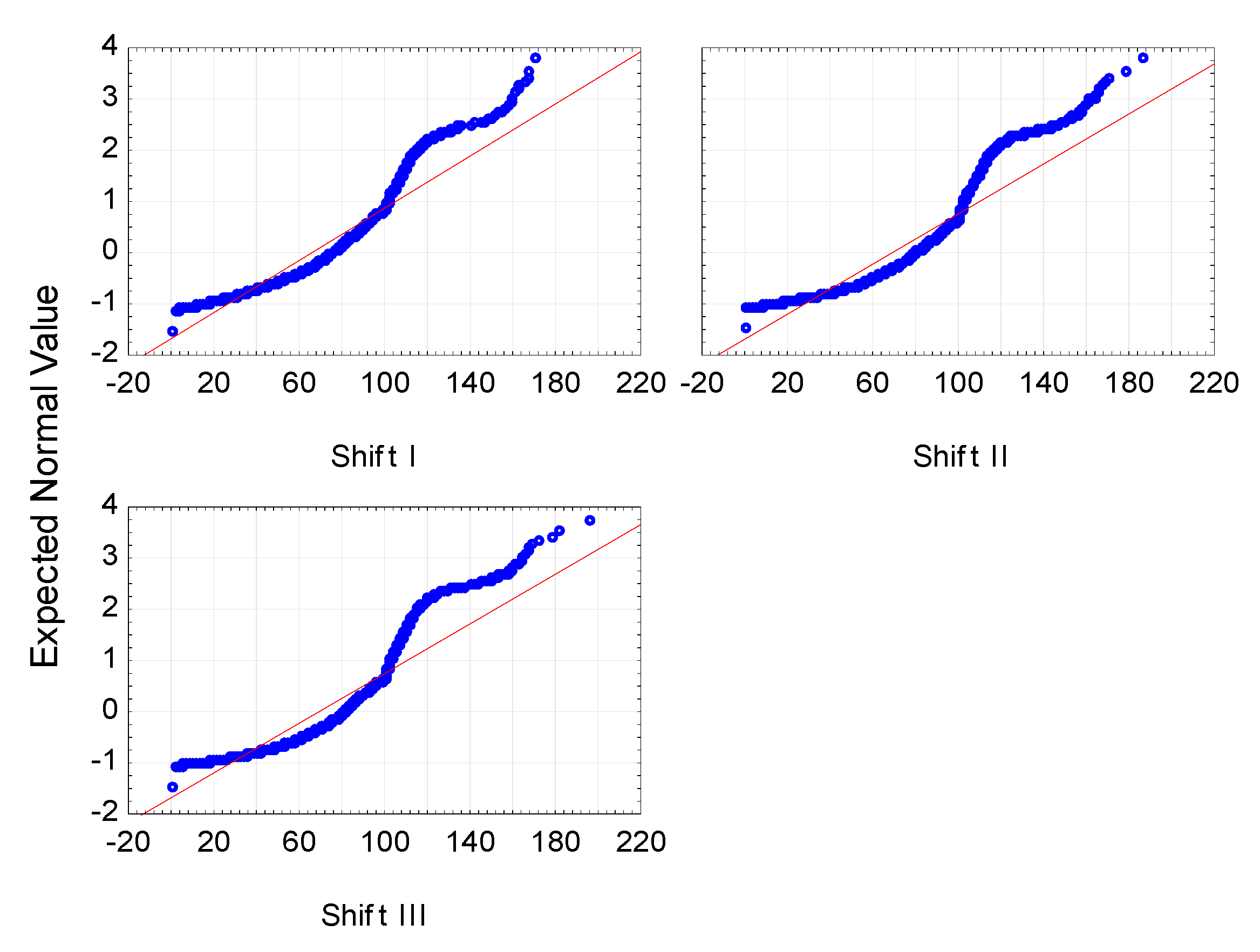
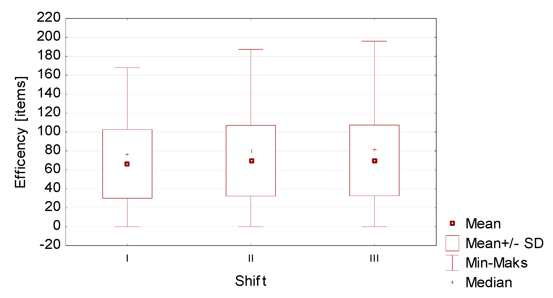
The shift predictor was analyzed first. First of all, the normality of distribution and homogeneity of the variance of the efficiency dependent variable during individual shifts was examined in order to determine the possible methods of statistical analysis. The distributions in all groups turned out to be inconsistent with the normal distribution, which is confirmed by the graphs in
Figure 1 and the calculated chi-square test statistic values, presented in
Table 1.
Next, the homogeneity of variance in individual groups was checked; the Levene and Brown-Forsythe test was used for this purpose. The obtained results are presented in
Table 2.
Although the homogeneity of variance was confirmed in all groups, due to the lack of normality of distributions, the Mann–Whitney test was used to examine the significance of differences between individual averages, and the results thereof are presented in
Table 3.
The analyses showed that there were no significant differences between the efficiency of the second and third shift, so a decision was made to combine them. However, the values obtained for the first shift differ significantly from those obtained for the other shifts, therefore this group was left without interference. These conclusions are confirmed by
Figure 2 showing the differences described.
The same test was performed for the device variable. The machines analyzed were of a single type and came from a single production batch, which suggests that their productivity would be similar. In order to confirm the equality of averages, the analysis of distribution normality and variance equality in individual groups (this time defined by the device variable) was carried out again in order to select a proper statistical distribution. The results of the normality test did not confirm the conformity. All the calculated chi-square test statistic values did not allow the zero hypothesis of the compatibility of the examined distribution with the normal one to be accepted. A definite deviation is confirmed by
Figure 3.
The analysis of the equality of variance using the Levene and Brown-Forsythe tests showed that variances are not equal in some groups. Consequently, the Mann–Whitney test was used to check the difference between averages, the results of which are presented in
Table 4.
Since the average efficiency varied for virtually every pair of devices, a decision was made not to combine them and to include each of them in the study. After defining the form of independent variables, the impact of each of them on the dependent variable, i.e., efficiency, was checked, but presented in a dichotomous form, as an assessment of whether the level achieved was satisfactory for the company. In line with the expectations of the Management Board, it was assumed that the assessment was positive if the productivity was equal to or above 90%. In other cases, the assessment would be negative. The chi-square test allowed for a statistical and substantive study of the relationship between variables. In all cases, the calculated test statistic did not allow the zero hypothesis on the lack of relationships between variables to be accepted. It was therefore rejected in favor of the alternative hypothesis of the existence of a relationship, the strength of which was measured using Yule’s Φ (for binary tables) and Cramér’s V coefficient (for tables more complex than 2 × 2). The obtained results are presented in
Table 5.
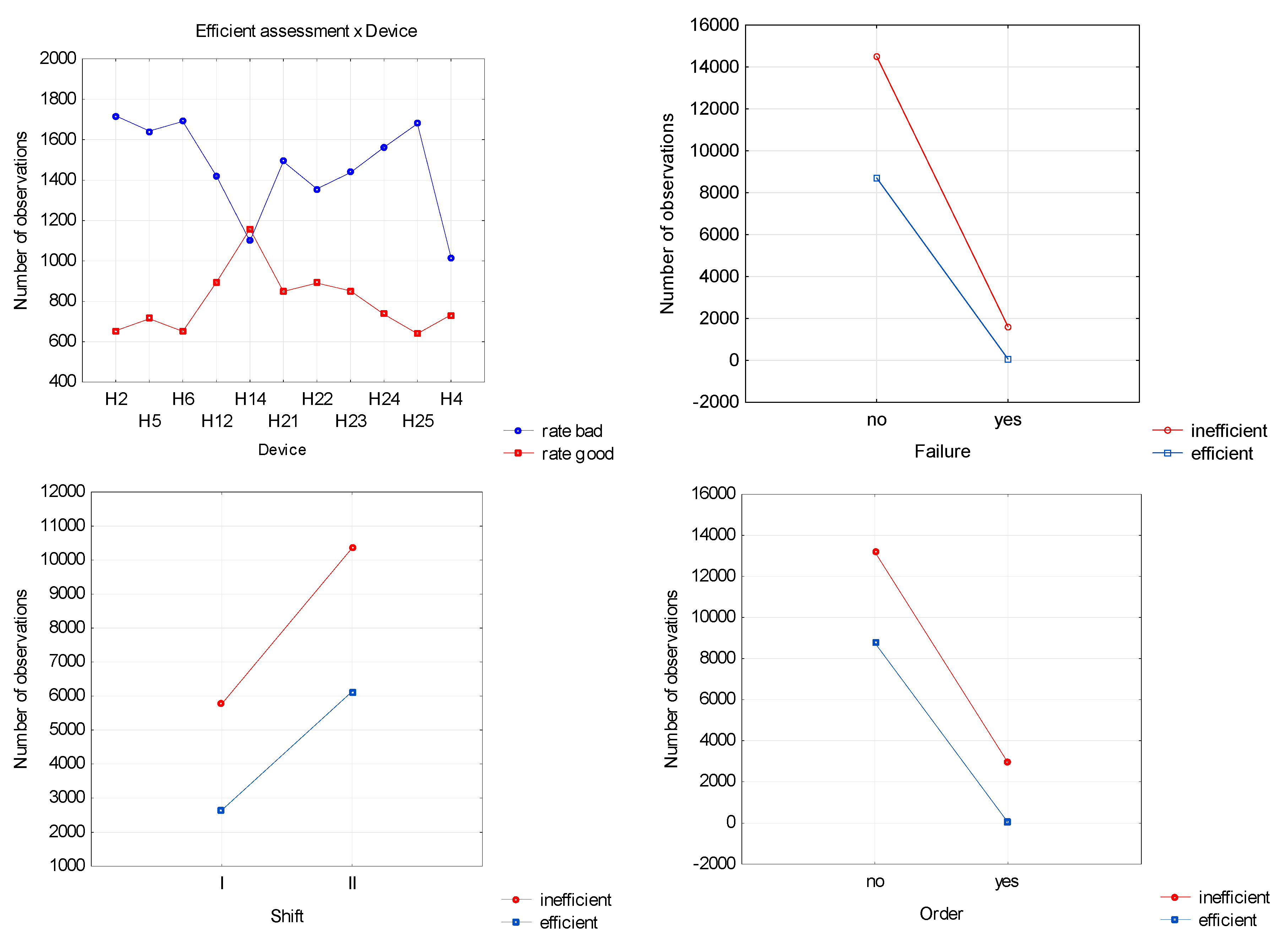
The observed relationships between variables, although significant, are not strong. This is also confirmed by the graphs of interaction of individual dependent variables with the explained variable (
Figure 4). Nevertheless, from the point of view of the analyzed company, the diagnosed bonds should not take place at all. A uniform and efficient operation of all devices is expected, so even minor deviations are undesirable and require further investigation.
The calculations carried out (
Table 5) and the charts (
Figure 4) confirm that the model variables were selected correctly. This allows the parameters of the logistic regression model to be estimated, the values of which are presented in
Table 6.
All calculated parameters turned out to be statistically significant, which is confirmed by the calculated Wald’s statistic value and the associated probability value
p, which for each line is lower than the assumed level of significance
. (
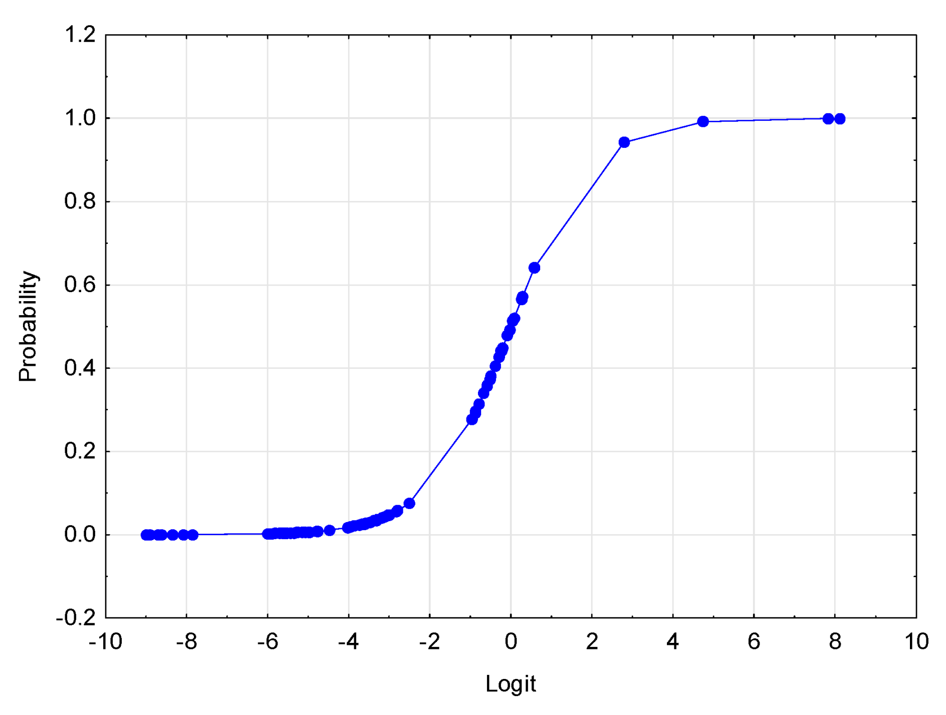
Table 6). This means that all the distinguished factors significantly affect the evaluation of production efficiency. This allows the equation of the logistic regression model to be written in the following form:
where
The logistic regression curve is shown in
Figure 5.
The logistic regression equation presented above can also take equivalent forms:
logistic regression logit function:
in the form of the odds:
where
An important element of the evaluation of the studied process is the calculation of the odds of an event occurrence (in this case a satisfactory result of efficiency). The sign at the estimated parameter of the logistic regression model indicates whether the analyzed odds are greater (plus) or smaller (minus) in relation to the reference level. The scale of this change is indicated by the unit odds ratio shown for each parameter in
Table 7.
The odds ratio for the 1st shift is 0.75, which means that compared to the 2nd shift, the odds of achieving satisfactory efficiency is 0.75 times lower. In other words, the odds for the proper efficiency is 1.34 times higher in the case of the 2nd shift. The H14 machine was used as a reference when analyzing the impact on the efficiency of individual devices. Its efficiency is the highest in the test sample, so all the model coefficients obtained are negative, which means less odds of achieving a positive result. The odds ratios are given in column 3 of
Table 6. The worst result was obtained for the H2 machine with an odds ratio of 0.289, which means an almost 3.5-fold increase in the odds of achieving satisfactory efficiency when replacing H2 with H14.
The results for the other machines, showing how much the efficiency of each machine should be increased in order to obtain the efficiency evaluation as in the case of the H12 machine, are shown in
Table 8.
The last two parameters in
Table 7 refer to the absence of an order or failure, as their occurrence has a negative impact on the efficiency. Where there is no downtime, the odds of achieving the expected efficiency are 155 times greater than otherwise. Similarly, the occurrence of a failure has a similar effect, but its absence is not as spectacular. There is a 21-fold increase in the odds if the failure does not occur.
The presented model can also be used for predictive purposes, allowing for forecasting the probability of achieving the predicted success (here, the assumed efficiency). It is therefore important to assess the quality of the prediction. For this purpose, it is helpful to determine the so-called cut-off point
. This parameter allows the observed dichotomous values of a dependent variable to be compared with the continuous probability values calculated on the basis of the model. This value falls within the range (0, 1) and is defined as follows [
36] when:
it is assumed that an event has occurred
. In the opposite situation, when
it is assumed that an event has not occurred
.
Prediction ideally occurs when sensitivity and specificity are equal to 1, which means no false positive or negative results. In real life research, the point corresponding to a case where a model best discriminates occurrences is called the optimal cut-off point. It is determined using the Youden’s index (
J), which takes the following form:
The optimum cut-off point corresponds to the case where the
J value reaches its maximum. For the case under consideration, the proposed cut-off point is shown in
Table 9.
For the proposed cut-off point, the sensitivity is 0.32, and the specificity is 0.86. There are 16,767 well classified cases (2864 true positive and 13,903 true negative) and 8115 badly classified cases (2210 false positive and 5905 false negative cases).
Based on the above table it is possible to assess the effectiveness of model prediction in relation to successes and failures, using tools among which one can distinguish such statistics as accuracy, sensitivity or specificity, ROC (receiver operating characteristic) curve or values of rank correlations.
The simplest measure is accuracy, calculated according to the following formula:
where:
TP—number of true positive results,
TN—number of true negative results,
FP—number of false positive results,
FN—number of false negative results.
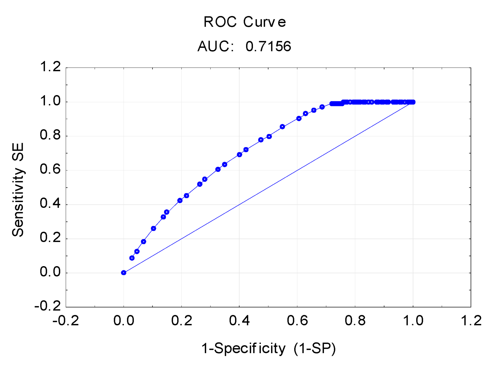
However, the sensitivity
SE and specificity
SP are most often considered in such analyses but treated as pairs, which, after being marked on the plane and after connecting the points with segments, form the so-called ROC curve. For the analyzed model this curve is presented in
Figure 6.
The most important parameter for assessing the ROC curve is AUC—area under the ROC curve. It takes values from 0 to 1. The interpretation of the result was based on the Kleinbaum and Klein classification (
Table 10), according to which discrimination is sufficient [
37].
The model can therefore be considered satisfactory, although it is recommended rather for qualitative analysis of processes and modification of production strategy on its basis.
Production in the company in question is carried out in a continuous three-shift system. Regardless of the production plan, the plant is fully manned and all machines are in operation at all times. The acceptable level of efficiency assumed by the management should be 90%, which allows all scheduled and expected downtime to be taken into account. The study indicates that in most cases this level is not reached. In almost 25,000 out of over 156,000 observations, this level was not reached. It turned out that the efficiency of the first shift was lower compared to the second and third ones, which suggests the need to diagnose the causes of circumstances or even to restructure the shift system. The use of individual machines also has a negative impact on efficiency. It turns out that many of them represent much lower efficiency than the one taken as a reference point, the efficiency of which was the highest (but also less than 100%). Of course, a lack of orders also leads to a significant reduction in productivity. Such a result, next to failures that occur, indicates the need for a detailed analysis of the machinery. It might be advisable to exclude several machines from the production process so that production is closely correlated with demand. Unused machines could constitute a reserve in case of failure and thus increase the level of readiness of the machinery.
4. Conclusions
The reliability of machinery and equipment is an essential part of the proper functioning of a business. Modern technologies support the maintenance of an adequate level of readiness and suitability of the technical infrastructure. They not only facilitate production control and implementation of modern operating strategies, but also ensure continuous monitoring of processes and detection of any disturbances or failures. The activities carried out in this area boil down to balancing the maintenance of full operational efficiency and continuity of production and ensuring an acceptable level of costs of these activities.
This is a difficult task, particularly in the case of older generation machinery stock, which is deprived of support from computerized production management systems—as the one presented in this article. In any case, however, the aim is to ensure that machines function perfectly without failures and that products are manufactured without defects. On the other hand, it is also important to ensure the efficiency of the equipment use and balanced workload, which proved to be a problem in the analyzed company. This was the reason for undertaking research in this field and the basis for mathematical analysis of the effectiveness of the manufacturing process.
The lack of IT systems for controlling and monitoring the production process results in the inability to archive data on an ongoing basis, which makes it much more difficult to control processes, and sometimes it is conducive to abandonment thereof. Poor quality of recorded documentation imposes significant limitations on the use of mathematical tools as well; therefore, the authors wanted to present simultaneously that even in such a situation it is possible to create mathematical models that would improve the efficiency of the machinery stock. The available data proved to be sufficient to achieve the research objective, which was to formulate a model providing an unambiguous answer as to whether the efficiency of the equipment used in production is acceptable from the point of view of the assumptions made by the company (in this case 90%).
This was made possible through the use of logistic regression, which, above all, does not require the meeting of assumptions made by other mathematical models, e.g., linear regression and general linear models. The advantage of this method is also the form of the dependent variable. The predictor here is a dichotomous variable and its values can be interpreted as the probability of an event occurring. The organization of production in the analyzed company has remained unchanged for many years. All machines work three shifts every day. Regardless of the orders placed and the market demand, full staff is employed. Machines are taken out of the process only in cases of random incidents. Lack of modification of the adopted procedures and control of the implemented processes results—as demonstrated in the research—in the process not being effective and the use of machinery not being optimal.
The logistic regression model made it possible to identify the causes influencing machinery efficiency. It turned out that the load is not identical during every shift, the productivity is much lower during the first shift in comparison to the other shifts. Restructuring the shift system and limiting the production process to only two shifts or modifying the working time could increase the productivity of machinery, optimize the use of human resources and reduce the costs of the production process. The load on the individual machines also appeared to be disproportionate. Increased use of one piece of equipment may result in an increase in the frequency of breakdowns, increase the costs of repairs and reduce the total life of the equipment, so it would be advisable to evenly distribute production across all equipment. The reduction in productivity was also caused by a decline in the number of production orders. The lack of production control with regard to orders received and the maintenance of a continuous three-shift readiness exposes the company to costs and favors the aforementioned disproportionate workload.
The studied company has no IT systems in place that enable comprehensive monitoring of production processes. Therefore, the unquestionable advantage of the proposed model is the provision of additional information allowing decisions to be made on the production and use of machinery. They can also encourage the implementation of modern solutions and the abandonment of traditional, outdated methods of recording and archiving data.
In companies that use specialist MES systems based on real-time information on manufacturing execution at subsequent workstations, the proposed model can improve monitoring of productivity drops below the adopted level and activate preventive actions. Additionally, the implementation of data obtained from the IT system may allow to the model to be extended with additional parameters, which is important from the point of view of individual companies.
The aim of the article was to investigate the possibility of developing a model for the analysis and evaluation of the level of efficiency of ongoing production processes, as well as to indicate the method of logistic regression as a tool supporting decision-making in this respect. The model developed for the analyzed company indicated the need for a strict correlation between the demand for a product and the production process. Adopted strategies require verification and modification.
The proposed model may also serve as a basis for setting directions for improvement of the production process, by maximizing the use of the machinery stock and reducing the idle time of both employees and equipment. Re-application of the logistic regression model constructed on the basis of the observation of the process after introduction of changes allows the effectiveness and efficiency of implemented solutions to be evaluated.


