Article

A Systematic Error Compensation Method Based on an Optimized Extreme Learning Machine for Star Sensor Image Centroid Estimation

1
Xi’an Institute of Optics and Precision Mechanics, Chinese Academy of Sciences, Xi’an 710119, China
2
University of Chinese Academy of Sciences, Beijing 100049, China
3
College of Geology Engineering and Geomatics, Chang’an University, Xi’an 710064, China
*
Author to whom correspondence should be addressed.
Appl. Sci. 2019, 9(22), 4751; https://doi.org/10.3390/app9224751
Submission received: 21 October 2019 / Revised: 3 November 2019 / Accepted: 4 November 2019 / Published: 7 November 2019

Abstract

:
As an important error in star centroid location estimation, the systematic error greatly restricts the accuracy of the three-axis attitude supplied by a star sensor. In this paper, an analytical study about the behavior of the systematic error in the center of mass (CoM) centroid estimation method under different Gaussian widths of starlight energy distribution is presented by means of frequency field analysis and numerical simulations. Subsequently, an optimized extreme learning machine (ELM) based on the bat algorithm (BA) is adopted to predict the systematic error of the actual star centroid position and then compensate the systematic error from the CoM method. In the BA-ELM model, the input weights matrix and hidden layer biases parameters are encoded as microbat’s locations and optimized by utilizing the strong global search capacity of BA, which significantly improves the performance of ELM in terms of prediction accuracy. The simulation result indicates that our method can reduce the systematic error to less than 3.0 × 10−7 pixels, and its compensation accuracy is two or three orders of magnitude higher than that of other methods for estimating a star centroid location under a 3 × 3 pixel sampling window.

1. Introduction

Reliable and accurate attitude determination plays a significant role in aerospace missions. Star sensors provide the most accurate three-axis attitude information when compared with other attitude measurement devices such as the sun sensor, magnetometer, and gyroscope [1,2]. Therefore, star sensors are widely equipped on orbiting satellites and interplanetary spacecraft [3,4,5]. Attitude estimation by star sensors proceeds by comparing star locations in the image taken by star sensors with those in the predefined on-board catalogue. The accuracy of estimating star centroid locations is one critical factor which directly affects the performance of the star sensor [6]. In this paper, we apply the extreme learning machine optimized by the bat algorithm (BA-ELM) to improve the star centroiding accuracy.
To solve the revolution limitation problem of the image plane, defocusing technology, expanding the star image spot to cover neighboring detector pixels, is adopted to obtain centroid precision at the subpixel level [7]. In the past 40 years, several subpixel centroid approaches [8,9,10] have been proposed. Among these existing methods, the center of mass (CoM) centroid estimation method features high speed and simplicity of calculation, so CoM is utilized in engineering projects. However, the location accuracy of the CoM method is influenced by two types of noise, namely, random noise and systematic noise.
Random noise, which contains dark current noise, short noise, radiation noise, etc., is related with the hardware system of the star sensor [11]. Systematic noise is caused by the character of the centroid estimation algorithm itself, and it brings about several arc seconds of accuracy loss in the star centroid location. In this paper, we focus on analyzing the systematic error in the CoM method, and then we propose a compensation method to remove the accuracy loss introduced by the systematic error, while the random noise is also discussed briefly.
Investigations into the systematic error in the CoM centroid estimation method have been made by several scholars. In general, the systematic error is related with the starlight energy distribution, the sampling window size, and the actual position of the detected star spot. Grossman et al. [12] found that the systematic error decreases when the starlight energy is defocused to wider neighboring pixels. Stanton et al. [13] pointed out that the relationship curve between the systematic error and the actual position of the star spot roughly satisfies a sinusoid pixel periodic function under fixed Gaussian width. Hancock et al. [14] supplemented Stanton’s work and studied the systematic error under different blur sizes of star spots, detector fill ratios, and pixel sizes numerically. Alexander et al. [15] studied the systematic error for the CoM centroid estimation method and gave a general expression for the systematic error. Rufino et al. [16] introduced a numerical model of the defocused point spread function, in which the defocus effects and diffraction were considered, and employed a backpropagation neural network (BP) to reduce the systematic error. Jia et al. [17] presented a theoretical analysis of the systematic error in the CoM method by a frequency field approach considering both the limitation of the detector sampling frequency and the limitation of the sampling window size, and they then proposed a compensation method based on the obtained analytical expression to improve the centroid accuracy. Zhang et al. [18] used the least square curve fitting method to estimate several key parameters in a bivariate polynomial model and developed a method utilizing a bivariate polynomial compensation template to correct the systematic error. Yang et al. [19] conducted least squares support vector regression (LSSVR) to eliminate the systematic error, where a trained LSSVR model was applied to predict the systematic error and then compensate for this error.
This paper presents an analysis of the systematic error in the CoM method under different Gaussian widths of starlight energy distribution utilizing a frequency field approach and numerical simulations, and it indicates that the systematic error consists of approximate error and truncation error. The approximate error results from the limitation of the detector sampling frequency, and it will exist in a star centroid estimation method when the maximum spatial frequency of the sensor image is larger than the detector sampling frequency; the truncation error appears under the condition that the Gaussian width of the starlight energy distribution is relatively large, causing the signal of the detected star to fall out of the range of the sampling window and to be truncated asymmetrically by the window. To eliminate systematic error, we propose a new compensation method based on the BA-ELM model, in which the input weights matrix and hidden layer biases in ELM are optimized by utilizing the search ability of BA to remove adverse effects of random parameters, and the optimal results can be used to enhance the stability and prediction accuracy of the network with a lesser number of hidden neurons. The simulation results demonstrate that the proposed method can eliminate the systematic error and achieve much higher compensation accuracy compared with other methods.
The remainder of the paper is structured as follows: In Section 2, the error in the CoM method is analyzed through frequency field analysis and numerical simulations. In Section 3, a detailed description of the proposed BA-ELM compensation method is presented. In Section 4, several simulations are performed to evaluate the BA-ELM compensation method. Finally, a summary of the main conclusions is outlined in Section 5.

2. Error Analysis of the Center of Mass Method

The CoM method is adopted by most star sensors to estimate the star centroid position with subpixel accuracy since it is easy to implement and exhibits better real-time performance. Therefore, the error of the CoM method is utilized for all discussions in this paper. When the CoM method is applied to digital images captured by the star sensor, the model of the method is described as
x ^ g = i = 1 n w x i I i i = 1 n w I i , y ^ g = i = 1 n w y i I i i = 1 n w I i
where ( x ^ g , y ^ g ) is the actual star centroid position, n w is the number of validated discrete pixels in the sampling window, and ( x i , y i ) and I i are the geometric center coordinates and the detected signal intensity, respectively, of the ith pixel.
From Equation (1), we can see that the centroiding accuracy of the CoM method is associated with three factors: the size of the sampling window, the coordinates of the validated pixel, and the corresponding detected signal intensity. The use of both the sampling window and the geometric center coordinates is the nature of the CoM method, while the uncertainty in the detected signal intensity is related to random noise caused by dark current noise, radiation noise, readout noise, etc. As a result, the error of the CoM method includes two parts, namely, the systematic error and the random error. The systematic error is derived from discrete approximation and sampling window truncation in the centroiding process, while the random error is introduced as image sensor noise.
Firstly, the random error resulting from uncertainty in the detected I i is analyzed in this section. Since there are various noises in the sensor image, the measured signal intensity I i of the ith pixel includes two components: the starlight intensity E i and the noise intensity σ I . According to the statement in Reference [15], the random error σ r a n d in the x direction of the CoM method can be given as
σ r a n d 2 = [ i = 1 n w ( x i x 0 ) ] 2 σ I 2 I 0 2 = ( σ I I 0 ) 2 i = 1 n w [ ( x i x 0 ) ] 2
where
I 0 = i = 1 n w I i ,   E 0 = i = 1 n w E i ,   x 0 = i = 1 n w x i E i / E 0 .
Through Equation (2), it can be seen that the σ r a n d value is determined by the signal-to-noise ratio (SNR), so improving the SNR, such as by optimizing the circuits or choosing low-noise image sensors, is an effective method to reduce the random error [20]. Scholars have proposed some methods to eliminate the random error, and further details concerning these are described in [12,21].
In this paper, we focus on the systematic error in the CoM method. The frequency field method and simulations are utilized to present an explicit analysis of the two types of error sources that bring about the systematic error, namely, the discrete approximation error and the sampling window truncation error.

2.1. Discrete Approximation Error

The star image sampling process includes three steps for star sensors, as illustrated in Figure 1. Firstly, the ideal star signal intensity function I(x) projected on the surface of the Charge-coupled Device (CCD) is convoluted with the pixel response function p(x) to generate the continuing pixel signal function f(x). Then, after multiplying the pixel sampling function s(x), f(x) is discretized and the corresponding sampled pixel signal function f s (x) is obtained. Finally, f s (x) is multiplied by the window response function r(x) to give the windowed pixel signal function g(x) utilized in star centroid estimation by the CoM method. The above process can be written as
g ( x ) = f ( x ) × s ( x ) × r ( x )
where
f ( x ) = I ( x , x 0 ) p ( x )
where I(x, x 0 ) denotes the ideal star signal intensity function with ideal centroid position x 0 in the x direction of the image plane.
We assume that the fill factor is 100%, pixel sensitivity is uniform, and each pixel in the image plane has the same photon response. Then, p(x) and r(x) are equal to the rectangle function rect(x), s(x) is equal to a comb function comb(x) with 1 / T sampling frequency (T is the length of a pixel), and Equation (4) can be written as
g ( x ) = I ( x , x 0 ) r e c t ( x T ) × c o m b ( x T ) × r e c t ( x n w T ) .
If we represent all distances in unit T, Equation (6) can be rewritten as
g ( x ) = I ( x , x 0 ) r e c t ( x ) × c o m b ( x ) × r e c t ( x n w ) .
In this section, we discuss the systematic error under the case where almost the complete sampled pixel signal f s (x) is included in the window, so f s (x) can be considered equivalent to g(x); then
g ( x ) = I ( x , x 0 ) r e c t ( x ) × c o m b ( x ) .
According to the properties of Fourier transform, the estimated centroid x ^ g is represented as follows [15]:
x ^ g = x g ( x ) d x g ( x ) d x = G ( 0 ) 2 π i G ( 0 ) .
where G(s) is the Fourier transform of g(x).
We set a pixel center as the coordinate system origin O; then the function f(x) of the star spot located at d can be expressed as the function f e (x) shifted by offset d from the origin O, i.e.,
f ( x ) = f e ( x d ) .
From Equations (5) and (10), we notice that d = x 0 . Thus, the Fourier transform of the function f(x) is
F ( s ) = exp ( 2 π i d s ) F e ( s ) .
where F e (s) is the Fourier transform of f e (x).
From Equations (8) and (11), G(s) is given as
G ( s ) = F ( s ) S ( s ) = exp ( 2 π i d s ) F e ( s ) S ( s ) .
where S(s) is the Fourier transform of s(x). Then, we have the derivative of G(s):
G ( s ) = F ( s ) S ( s ) = [ 2 π i d exp ( 2 π i d s ) F e ( s ) + exp ( 2 π i d s ) F e ( s ) ] S ( s ) .
Substituting Equations (12) and (13) into Equation (9) yields
x ^ g = G ( 0 ) 2 π i G ( 0 ) = d exp ( 2 π i d s ) F e ( s ) S ( s ) 2 π i exp ( 2 π i d s ) F e ( s ) S ( s ) | s = 0 .
Therefore, the systematic error is obtained as
σ x ^ g = x ^ g x 0 = 1 2 π i n = exp ( 2 π i d n ) F e ( n ) n = exp ( 2 π i d n ) F e ( n ) .
Equation (15) is the general expression of the systematic error in the CoM method considering only the sampling frequency limitation. Then, we can derive a more explicit relationship by substituting the specific function f(x) of the star spot in the image sensor into the above equation.
The detected star is viewed as a point source for star sensors, and it usually covers a certain pixel region in the actual star images due to the defocus measure. Therefore, a Gaussian function is a reasonable approximation to describe the signal blurring effect [7,22], and the 2-D signal intensity distribution of the star spot can be written as
I ( x , y , x 0 , y 0 ) = I 0 2 π σ P S F 2 exp [ ( x x 0 ) 2 + ( y y 0 ) 2 2 σ P S F 2 ] .
where I 0   is the total energy of the starlight, ( x 0 , y 0 ) is the ideal star centroid position, and σ P S F is the Gaussian width. For the 1-D case, Equation (16) can be reduced to
I ( x , x 0 ) = I 0 2 π σ P S F exp [ ( x x 0 ) 2 2 σ P S F 2 ] .
Since I(x, 0) is an even function, the function f e (x), which is the convolution result of I(x, 0) and p(x), is also even. Thus, we have
σ x ^ g = 1 π n = 1 sin ( 2 π n x 0 ) F e ( n ) F e ( 0 ) + 2 n = 1 cos ( 2 π n x 0 ) F e ( n ) .
From Equation (5), it follows that
F e ( s ) = { f e ( x ) } = { I ( x , 0 ) r e c t ( x ) } = I 0 exp [ 2 ( π s σ P S F ) 2 ] sin ( π s ) / π s .
where { } denotes the Fourier transform operation. Then
F e ( n ) = I 0 exp [ 2 ( π σ P S F n ) 2 ] cos ( π n ) / n = ( 1 ) n I 0 exp [ 2 ( π n σ P S F ) 2 ] / n .
Therefore, the theoretical expression of the systematic error with a Gaussian distribution of starlight energy can be written as
σ x ^ g = 1 π n = 1 ( 1 ) n exp [ 2 ( π n σ P S F ) 2 ] sin ( 2 π n x 0 ) / n .
Actually, when the condition σ P S F > 0.2 is satisfied, exp[−2 ( π σ P S F ) 2 ] exp[−2 ( π n σ P S F ) 2 ] (n 2); then Equation (21) is simplified to
σ x ^ g = 1 π exp [ 2 ( π σ P S F ) 2 ] sin ( 2 π x 0 ) .
Equation (22) indicates that the relationship between σ x ^ g and x 0 can be described as a sinusoid function under sampling frequency limitation. Moreover, the amplitude of σ x ^ g   decreases exponentially as the Gaussian width σ P S F   increases. To obtain the relationship in an actual situation, numerical simulations were performed in the following part.
During the experiment, the sampling window was fixed at 3 × 3 pixels, and the ideal point spread function (IPSF) model [23] was utilized to simulate a space discretized digital gray star image spot, that is, the signal intensity detected by the ith pixel was
I i = x i 1 / 2 x i + 1 / 2 I ( x , x 0 ) d x .
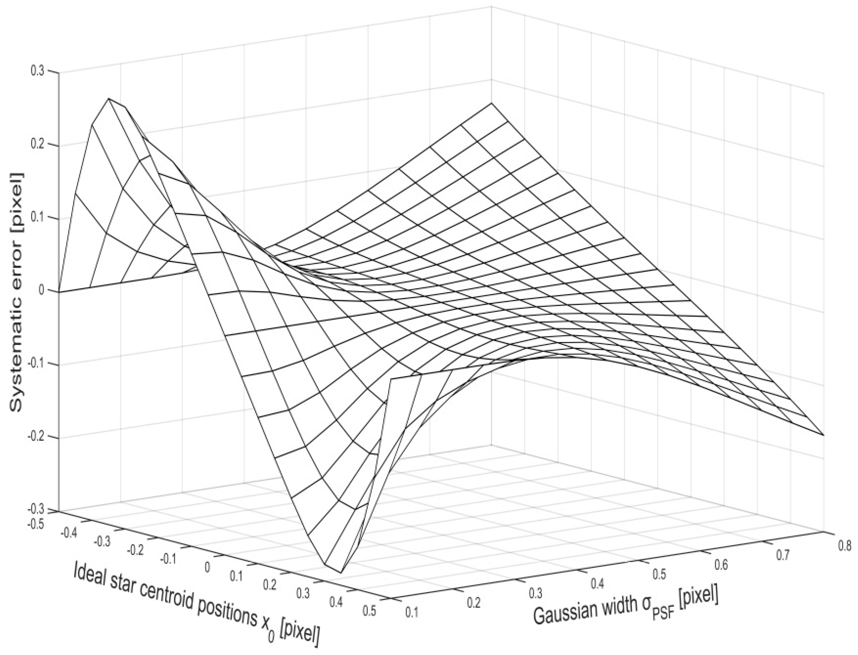
After drawing a group of relationship curves between σ x ^ g and x 0 under the different Gaussian widths, the corresponding 3-D numerical simulation results are illustrated in Figure 2.
In Figure 2, there is an approximately sinusoid relationship when the Gaussian width σ P S F is at a small value ( σ P S F < 0.3 pixels), and the numerical simulation results are also consistent with the expression in Equation (22). The relationship curve tends to be linear when the Gaussian width σ P S F is relatively large ( σ P S F > 0.6 pixels), which results from the appearance of truncation error caused by the limitation of the sampling window size; this will be discussed in detail in the next section.

2.2. Sampling Window Truncation Error

From Equations (21) and (22), we can see that the systematic error in the CoM method will be reduced by increasing the Gaussian width of the star spot when only considering the sampling frequency limitation. Nevertheless, the received starlight energy becomes weaker for a pixel as the Gaussian width increases, which results in deterioration of the SNR of the star image, resulting in greater random error. Therefore, a sampling window is utilized to limit the number of pixels around the actual star spot. When the sampling window size is relatively small, starlight energy falls out the window, and the signal of the detected star may be truncated asymmetrically; this causes a truncation error. Figure 3 illustrates how window truncation leads to error in the centroid calculation process.
In Figure 3a, it can be seen that the discrete star spot signal function e(k) detected by CCD pixels occupies about four pixels in the image plane, while the width of the sampling window is only three pixels (Figure 3b); as a result, the discrete signal function e(k) is truncated asymmetrically when the pixel detected signal is multiplied by the window response function. As shown in Figure 3c, the partial pixel detected signal in e(k) located outside the sampling window r(x) will be excluded in calculating the star centroid position. The nonsymmetrical truncation causes the estimated centroid x ^ g to be smaller than the ideal centroid x 0 , that is, a truncation error is introduced into the final estimated results of the CoM method.
Here, we analyze the numerical simulation results under Gaussian widths σ P S F of 0.3 and 0.671 pixels to present the influence of the truncation error on the relationship curve of σ x ^ g and x 0 .
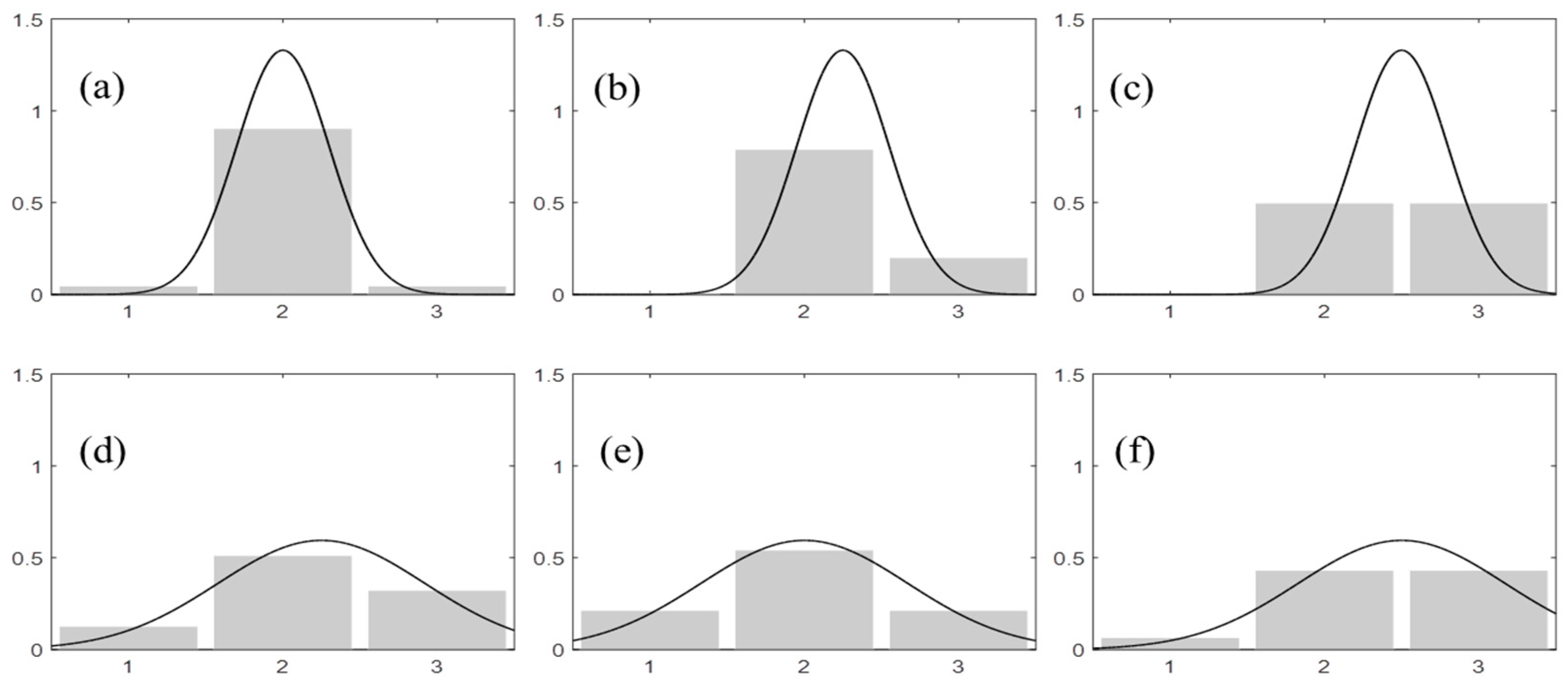
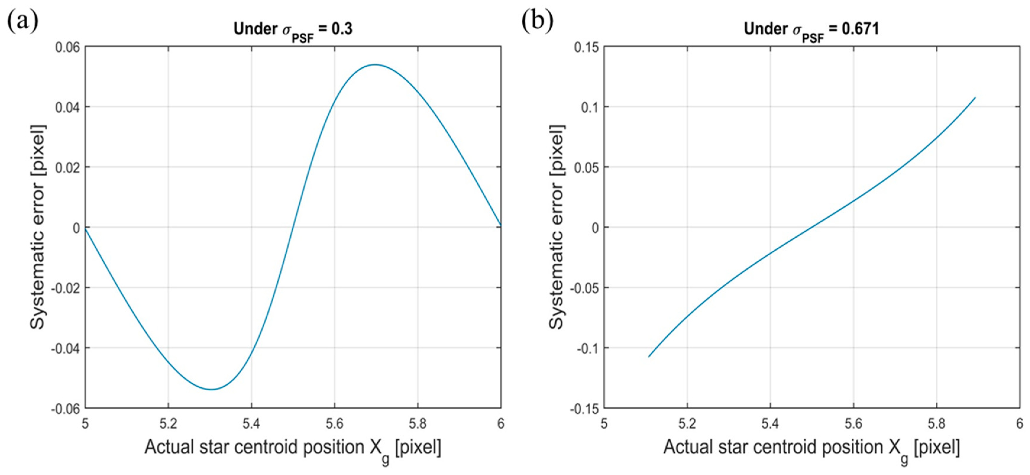
Figure 4 shows the respective pixel detected signals in the three-pixel sampling window when the ideal star centroid positions are x 0 = 2, 2.25, 2.5 under Gaussian widths σ P S F = 0.3, 0.671 pixels. We can see that the complete pixel detected signal is included in the sampling window with σ P S F = 0.3 pixels during the process of moving the star centroid from the pixel center to the edge (Figure 4a–c), since the width of the effective pixel detected signal is less than three pixels when σ P S F is at a small value. In this case, the pixel detected signal will not be truncated asymmetrically by the sampling window; thus, the systematic error is associated with the discrete approximation error, and the relationship curve between σ x ^ g and x 0 is sinusoid (Figure 5a). However, for the pixel detected signal with σ P S F = 0.671 pixels, the width is relatively lager than three pixels. As a result, the detected signal is truncated asymmetrically when it locates at a non-central position of the pixel, as shown in Figure 4e,f. Under this condition, the systematic error is mainly determined by window truncation error, the relationship curve becomes linear (Figure 5b), and the maximum error value appears when the star centroid is located at the pixel edge.

3. Materials and Methods

The key to compensating systematic error in the CoM method lies in predicting the corresponding systematic error σ x ^ g of the actual star centroid position x ^ g accurately and rapidly. Researchers have proposed several compensation methods in recent years, such as the BP method [16], analytical compensation (AC) method [17], bivariate polynomial method [18], and LSSVR compensation method [19], and they can reduce the systematic error to some extent, but there are some shortcomings in the compensation model of these methods. For example, the poor performance indices and low learning rate of the BP algorithm, along with how easily it becomes trapped in a local optimum, limit the compensation accuracy of this method; the simplified approximation and iteration estimation in the analytical compensation method lead to a reduction in the prediction accuracy and high on-line computational complexity, which is not suitable for the on-orbit embedded system; the bivariate polynomial compensation template is valid only for some specific Gaussian width cases, and its application range is thus limited; and the problem of scientifically setting the penalty factor and kernel parameter in LSSVR still remains unsettled, meaning that model training is more difficult because of a time-consuming parameter selection process.
ELM [24,25] has attracted attention in robot control [26], human face recognition [27], medical diagnosis [28], sales forecasting [29], and protein structure prediction [30] fields, among others, due to its simple training process and excellent generalization ability when compared to other traditional algorithms [31]. However, the randomness of input weights and hidden layer biases become a bottleneck restricting the stability and prediction accuracy of the ELM network. In order to overcome the adverse effects of extreme learning parameters and improve the performance of compensation methods, a systematic error compensation method based on BA-ELM is given herein to eliminate the systematic error of the star centroiding method considering both compensation accuracy and on-line computational load; the BA-ELM model is utilized to predict the systematic error and then improve the accuracy of the CoM method.

3.1. Extreme Learning Machine

Figure 6 shows the ELM network structure, which is formed by three layers: the input layer with n nodes, the hidden layer with L nodes, and the output layer with m nodes. The neurons in adjacent layers are fully linked. The input weight values and hidden layer biases in ELM are set randomly, and the activation function in the hidden layer maps the input space onto a new space, then a linear combination is performed on the new space. Thus, the parameter which has to be solved is the weight matrix that links the hidden and output neurons, which can be determined through the least square approach.
Given N training samples ( x i , t i ) , i = 1, 2, …, N, in which x i = [ x 1 i ,   x 2 i , ,   x n i ] T is an n-dimensional input vector of the ith sample and t i = [ t 1 i ,   t 2 i , ,   t m i ] T is an m-dimensional target vector associated with x i , the mathematical model can be written as
o i = j = 1 L β j g h ( w j x i + b j ) i =   1 ,   2 ,   3 ,   ,   N .
where o i = [ o 1 i ,   o 2 i , ,   o m i ] T is the m-dimensional output vector of the network with input vector x i , β j = [ β j 1 ,   β j 2 , , β j m ] T is the weight vector between the jth hidden neuron and the output layer, w j = [ w j 1 ,   w j 2 , , w j n ] T is the weight vector between the jth hidden neuron and the input layer, b j is the bias parameter of the jth hidden neuron, w j ·   x i denotes the inner product of w j and x i , and g h (x) is the activation function in the hidden layer.
According to the theory proposed by Huang [21], the ELM can approximate all given training samples without error, which implies that there are w j , b j , and β j   such that
j = 1 L β j g h ( w j x i + b j ) = t i i   =   1 ,   2 ,   3 ,   ,   N .
Equation (25) can be written in a linear system as
H β = T .
where H is the output matrix of the hidden layer and is defined as
H = [ g h ( w 1 x 1 + b 1 ) g h ( w 2 x 1 + b 2 ) g h ( w L x 1 + b L ) g h ( w 1 x 2 + b 1 ) g h ( w 2 x 2 + b 2 ) g h ( w L x 2 + b L ) g h ( w 1 x N + b 1 ) g h ( w 2 x N + b 2 ) g h ( w L x N + b L ) ] N × L .
β = [ β 1 T β 2 T β L T ] L × m and T = [ t 1 T t 2 T t N T ] N × m , where β is the weight matrix connecting the hidden layer and the output layer, and T is the target output matrix.
After assigning the coefficient matrices for random parameters, the matrix β can be estimated analytically by finding the minimum norm least squares solution:
β ^ = arg min β H β T = H + T .
where H + is the Moore–Penrose generalized inverse of H.

3.2. Bat Algorithm

The BA was proposed by Cambridge University scholar Yang [32] and has been approved as a useful method to solve the optimization problem. The principle of BA lies in the echolocation behavior of the microbats. The microbats emit sound pulse, and the sound pulse will be bounced back when it hits objects; then, bats listen for the echoes to estimate the surrounding scenario and search for their prey.
We assume that the microbats pursue the optimal solution in a d-dimensional space, and the velocity and location of the ith bat at step t are v i t and x i t , respectively. Then the updated velocity v i t + 1 and location x i t + 1 at step t + 1 are given by
x i t + 1 = x i t + v i t + 1 .
v i t + 1 = v i t + ( x i t x ) × F i .
where x * is the current global best solution in the bat group. F i is the frequency of the sound pulse emitted by the ith microbat, and it can be obtained as shown in Equation (31):
F i = F min + ( F max F min ) × μ .
where F max , F min are the maximum and the minimum sound frequency of the microbat.
After selecting a solution from the current best solutions, each bat performs a local search and produces a related new solution x n e w utilizing the random walk according to Equation (32):
x n e w = x o l d + ε × A t .
where A t is the average loudness of the sound pulse of the microbats at step t.
If the new solution is better than the current best solution, it will be accepted as an optimal solution with a certain probability. Meanwhile, the emission rate r i t and loudness A i t of the ith microbat at step t + 1 are updated by
A i t + 1 = α × A i t .
r i t + 1 = r i 0 × ( 1 exp ( γ × t ) ) .
where α and γ are constants and 0 < α < 1, γ > 0.
Based on the above description of BA, its pseudo code is shown in Algorithm 1. In fact, BA is much superior to other popular metaheuristic approaches such as particle swarm optimization (PSO), genetic algorithm (GA), and Harmony search [32]. Therefore, due to its strong ability in searching for optimal solutions, BA is utilized in engineering and industrial applications.
Algorithm 1. The pseudo code of the bat algorithm.
Initialize the bat population xi and vi (i = 1, 2, …, n)
Initialize frequencies Fi, pulse rates ri and the loudness Ai
while (t < max number of iterations)
  Generate new solutions by adjusting frequency, update velocities and locations
  if (rand > ri)
    Select a solution among the best solutions
    Generate a local solution around the selected best solution
  end if
  Generate a new solution by flying randomly
  if (rand < Ai & f(xi) < f(x*))
    Accept the new solutions
    Increase ri and reduce Ai
  end if
    Rank the bats and find the current best x*
end while

3.3. Optimized Extreme Learning Machine

The random selected parameters in the basic ELM may cause unacceptable prediction results and poor stability of the network [33,34,35]. To promote prediction accuracy, the parameters were coded as the microbat locations, with the corresponding fitness values being the root-mean-square error (RMSE) between the prediction value and actual value. BA was utilized to search for the optimal parameter combination during off-line training. The fundamental steps of BA-ELM are summarized as follows:
Step 1: Define the computational parameters relating to BA in the BA-ELM model, such as the maximum iteration number N_max and population size P_num.
Step 2: Define the ELM neutral network structure and the activation function g h (x).
Step 3: Set k = 1. The population set is randomly generated as the initial locations for the microbat group, in which each location of a bat possesses all random parameters. The position of the ith bat in the kth generation is denoted by θ i ( k ) and defined as
θ i ( k ) = [ w 1 , ( i , k ) , , w j , ( i , k ) , , w L , ( i , k ) , b 1 , ( i , k ) , , b j , ( i , k ) , , b L , ( i , k ) ] .
where b j , ( i , k ) and w j , ( i , k )   are the biases and input weights, respectively, of the jth hidden node for θ i ( k ) .
Step 4: Determine the output weights through Equations (36) and (37), and then evaluate the fitness value of the position of θ i ( k ) by Equation (38):
β ^ ( i , k ) = H ( i , k ) + T .
H ( i , k ) = [ g h ( w 1 , ( i , k ) x 1 + b 1 , ( i , k ) ) g h ( w 2 , ( i , k ) x 1 + b 2 , ( i , k ) ) g h ( w L , ( i , k ) x 1 + b L , ( i , k ) ) g h ( w 1 , ( i , k ) x 2 + b 1 , ( i , k ) ) g h ( w 2 , ( i , k ) x 2 + b 2 , ( i , k ) ) g h ( w L , ( i , k ) x 2 + b L , ( i , k ) ) g h ( w 1 , ( i , k ) x N + b 1 , ( i , k ) ) g h ( w 2 , ( i , k ) x N + b 2 , ( i , k ) ) g h ( w L , ( i , k ) x N + b L , ( i , k ) ) ] N × L .
F [ θ i ( k ) ] = 1 N s = 1 N ( t s o s ) 2 = 1 N s = 1 N [ t s j = 1 L β j g h ( w j , ( i , k ) x i + b j , ( i , k ) ) ] 2 .
where t s and o s   are the target value and output value, respectively, of the sth training sample, H ( i , k ) is the output matrix for θ i ( k ) , and H ( i , k ) + is the Moore–Penrose generalized inverse of H ( i , k ) .
Step 5: Initialize the location θ i and fitness value F i t [ θ i ] of the ith bat as θ i ( k ) and F[ θ i ( k ) ], respectively, in which k = 1.
Step 6: Set k = k + 1, i = 1. If the maximum iteration N_max is reached, go to Step 12; otherwise, go to Step 7.
Step 7: Generate the new location θ i ( k ) for the ith bat with Equations (29)–(31).
Step 8: Evaluate the fitness value F[ θ i ( k ) ] for the new location θ i ( k ) with Equations (36)–(38).
Step 9: Update the location θ i and fitness value F i t [ θ i ] of the ith microbat as θ i ( k ) and F[ θ i ( k ) ] if Equation (39) is satisfied. Otherwise, θ i and F i t [ θ i ] remain unchanged.
{ r a n d A i F [ θ i ( k ) ] F i t [ θ i ] .
Here, rand is a random number in [0, 1] and A i is the loudness of the sound pulse of the ith microbat.
Step 10: Find the current best location among the microbats.
Step 11: Set i = i + 1. If the population size P_num is reached, go to Step 6; otherwise, go to Step 7.
Step 12: Export the optimized ELM neutral network.

3.4. BA-ELM for Systematic Error Compensation

The BA-ELM model was utilized as the estimating function in our systematic error compensation method. In practice, the ideal star centroid position x 0 in the captured image cannot be obtained, but we can calculate the actual star centroid position x ^ g by the CoM method. According to Equation (24), the functional relationship between σ x ^ g and x ^ g estimated by BA-ELM can be written as
σ x ^ g = j = 1 L β j g h ( w j * x ^ g + b j * ) .
where w j * and b j * are the optimal parameters in the ELM obtained by BA. In practical operations, if we input x ^ g   into the BA-ELM model, it will output the corresponding predicted systematic error δ B A E L M ( x ^ g ), and then we have the compensated position x ^ g c by Equation (41). Through this way, the systematic error of the CoM method can be eliminated to the maximum extent.
x ^ g c = x ^ g δ B A E L M ( x ^ g ) = x ^ g j = 1 L β j g h ( w j * x ^ g + b j * ) .

4. Simulations and Discussion

In this section, experiments were conducted to evaluate the capacity of the proposed BA-ELM compensation method. The experiments included three steps. Firstly, we collected training samples before employing the BA-ELM to estimate the function. Secondly, some parameters which have an impact on estimating function performance were determined. The cross-validation method was utilized to optimize these parameters and obtain the BA-ELM model whose fitting accuracy and prediction accuracy met the requirements. Thirdly, we used the simulated star images to validate the BA-ELM systematic error compensation method in improving the accuracy of the CoM method. Finally, the performance of our method and that of other compensation methods were compared and discussed. All these simulations were written in Matlab R2015a and performed on an Intel Core 3.4 GHz computer.

4.1. Preprocessing the Sample Data

To estimate the relationship between the ideal star centroid position x 0 , the actual star centroid position x ^ g , and the systematic error σ x ^ g under the different Gaussian widths through the BA-ELM method, we devised a numerical simulation method to obtain the relationship function among them. In this paper, the sampling window was set to be 3 × 3 pixels, and two situations were simulated. The first case was when σ P S F is smaller than the size of the sampling window, in which the systematic error is only caused by approximation error. The second case was when σ P S F becomes larger than the size of the sampling window, and the systematic error includes both approximation error and truncation error. Thus, σ P S F was set to be 0.3 and 0.671 for these cases, respectively. The same method can be employed to obtain the compensation template and eliminate the systematic error under different Gaussian widths.
In our experiment, the star spot was projected onto the position (5, 7) of the image plane, and the star centroid position in the x direction ranged from 5 to 6. The pixel was subdivided evenly into 1000 parts, so the ideal star centroid position x 0 was 5.0001, 5.0002, 5.0003, ···, 6, that is, the simulation step was 0.001 pixels. In each simulation step, the actual star position x ^ g and its systematic error σ x ^ g defined in Equation (15) were recorded. The 1000 samples were acquired to estimate the relationship function between x ^ g and σ x ^ g when the Gaussian width was 0.3 or 0.671, as shown in Figure 7a,b, respectively, and they were used as input training samples for the BA-ELM model.
In Figure 7, the maximum systematic error was 0.054 pixels when σ P S F was 0.3, while under the condition σ P S F = 0.671, the maximum systematic error increased to more than 0.1 pixels, which is large enough to degrade the star sensor performance. We proposed the BA-ELM compensation method to decrease the systematic error. The 1000 samples were utilized to train the BA-ELM to estimate the relationship curves, and then the fitting accuracy and prediction accuracy were calculated in order to evaluate the BA-ELM compensation method.

4.2. The Fitting Accuracy of the BA-ELM

There are some key parameters influencing the BA-ELM performance, such as the hidden neuron number (HN_num), activation function g h (x), population size (P_num), and iteration number (N_max). During the process of optimizing the parameters, the RMSE in N training samples was adopted as the evaluation criterion:
R M S E = 1 N i = 1 N ( x ^ g x 0 δ B A E L M ( x ^ g ) ) 2 = 1 N i = 1 N ( x ^ g x 0 j = 1 L β j * g h ( w j * x ^ g + b j * ) ) 2 i = 1 , 2 , 3 N .
where δ B A E L M ( x ^ g ) denotes the prediction output of the BA-ELM with input x ^ g .
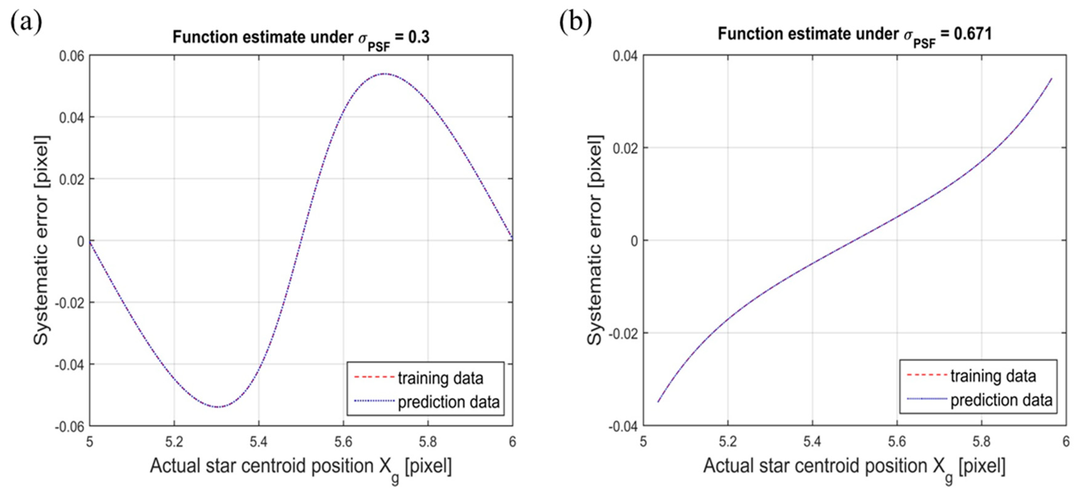
In consideration of the accuracy and computation time of the BA-ELM for estimating the function, we set HN_num = 25, P_num = 25, and N_max = 50 in the model. The prediction accuracies of the sig activation function and the sin activation function were compared by calculating their RMSE values, and the RMSE of the sin function was larger than that of the sig function by two orders of magnitude, so the sig function was selected as the activation function g h (x). Figure 8 shows the performance of the BA-ELM in the function estimation.
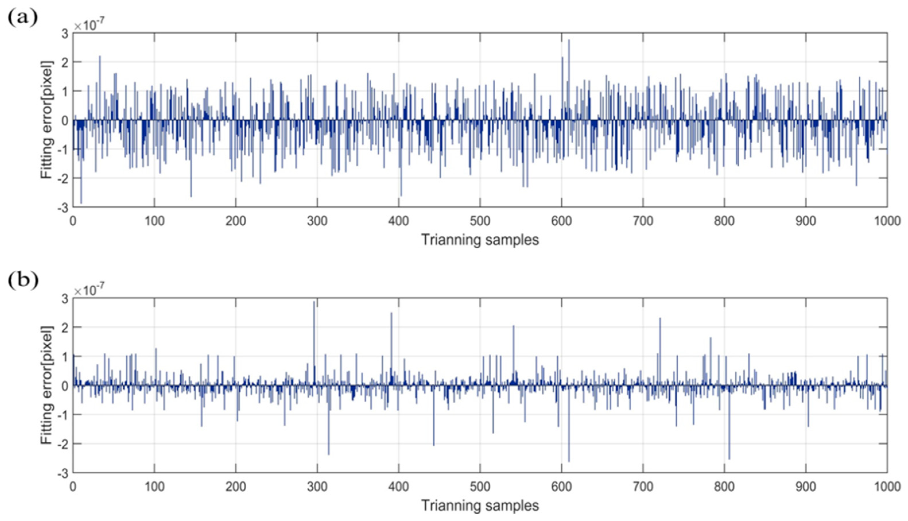
The relationship functions in Figure 8 almost overlap with the fitting curves estimated by the BA-ELM model; this illustrates that the BA-ELM can achieve excellent fitting accuracy under Gaussian widths σ P S F of 0.3 and 0.671. Detailed results on the fitting errors of the BA-ELM model are shown in Figure 9. Here, we defined the fitting error as the difference between the actual systematic error σ x ^ g and the predicted systematic error δ B A E L M ( x ^ g ) at the sampling positions. From Figure 9, it can be seen that when the σ P S F values were 0.3 and 0.671, the maximum fitting errors were 2.75 × 10 7 pixels and 2.88 × 10 7 pixels—both smaller than 3 × 10 7 pixels.

4.3. The Prediction Accuracy of the BA-ELM

The high fitting accuracy in the training samples cannot illustrate the performance of the BA-ELM model comprehensively. In practical operations, the BA-ELM is to be utilized to predict the systematic error of the star centroid at random positions. Therefore, the prediction accuracy is a critical parameter to evaluate the BA-ELM model. Firstly, the prediction accuracy is defined in this section.
Let x ^ g be the actual star centroid position obtained by the CoM method, and let δ B A E L M ( x ^ g ) be the predicted systematic error of the BA-ELM model with input x ^ g ; we have the compensated star centroid x ^ g c as
x ^ g c = x ^ g δ B A E L M ( x ^ g ) .
Then, the prediction error ξ of the BA-ELM model can be expressed by the following equation:
ξ = x ^ g c x 0 .
where x 0 is the ideal star centroid position.
After obtaining a trained BA-ELM model with optimal parameters, its prediction accuracy was calculated. In the simulations, 600 positions on the image plane were selected randomly, and then we made a star spot centroid traverse these positions sequentially. The coordinates in the x direction of these selected positions ranged from 1 to 512.
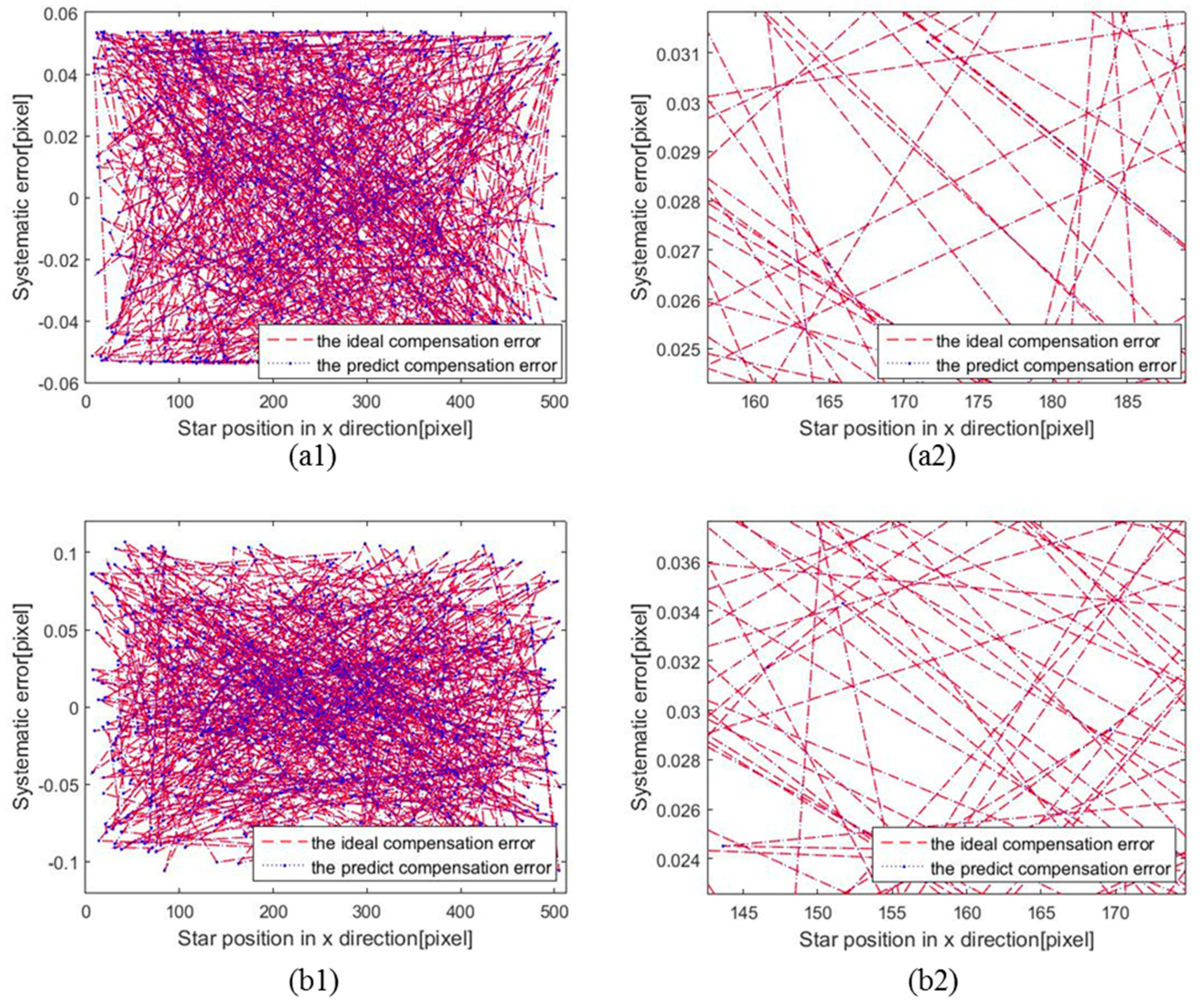
Figure 10 shows the respective results of the prediction accuracy in the 600 random positions under σ P S F = 0.3 and σ P S F = 0.671. The red lines were formed by connecting all ideal coordinates ( x 0 ,     σ x ^ g ) successively, while the blue lines were formed by connecting the compensated coordinates ( x ^ g c ,   δ B A E L M ( x ^ g ) ) . From Figure 10a2,b2, which are enlarged pictures relative to Figure 10a1,b1, we can see that the blue lines nearly the overlap red lines; this means that each compensated star position x ^ g c is extremely close to its corresponding ideal position x 0   in all test positions. The prediction error is illustrated in Figure 11.
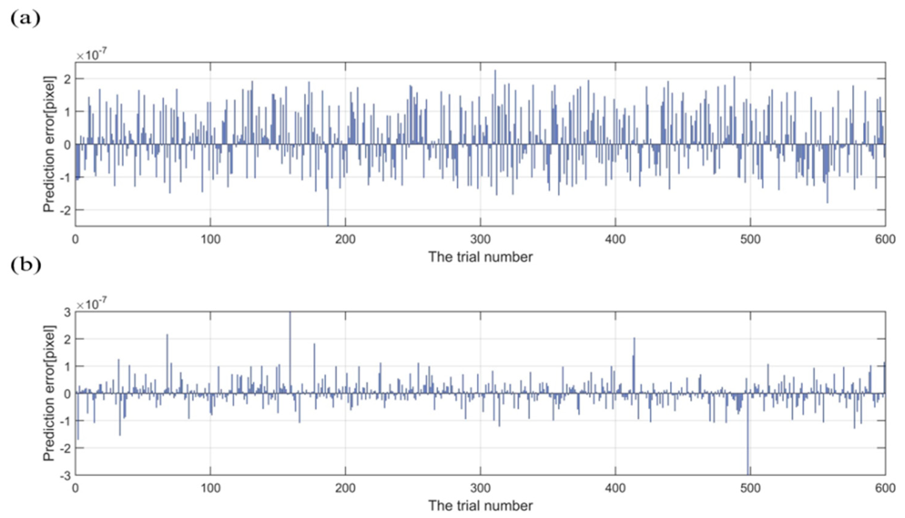
As shown in Figure 11, the maximum prediction errors of the BA-ELM were 2.5 × 10−7 pixels and 3.0 × 10−7 pixels when the σ P S F values were 0.3 and 0.671, respectively. The test results indicate that the proposed compensation method based on the BA-ELM model can achieve excellent prediction accuracy under different Gaussian widths.

4.4. The Compensation Performance in Star Images

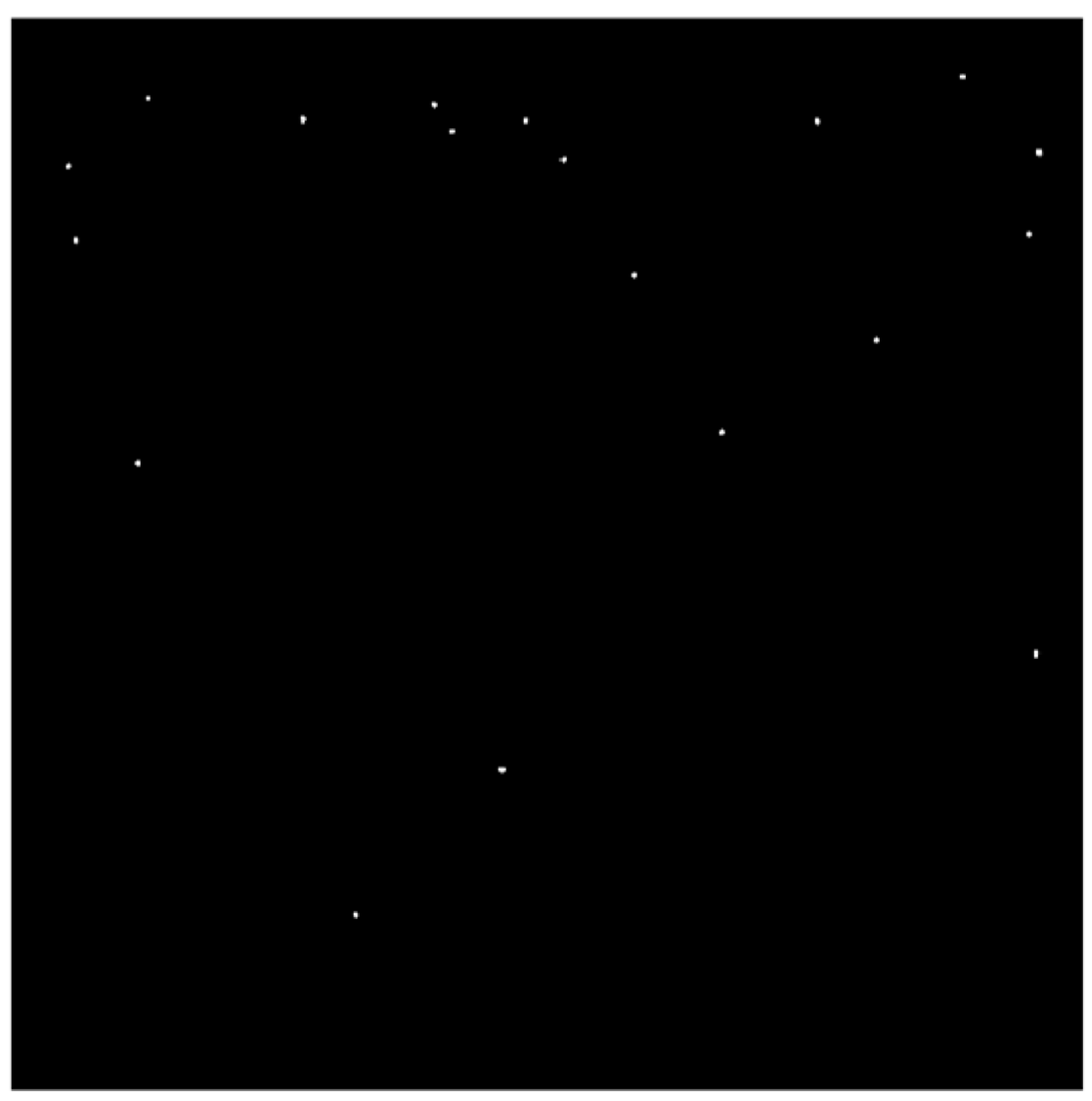
After evaluating the compensation performance on single star spots, we tested the BA-ELM compensation method on a simulated star image. For the simulations, the configuration of the star sensor is shown in Table 1, the field of view (FOV) direction was selected randomly, and the Smithsonian Astrophysical Observatory (SAO) J2000 star catalog was used to synthesize star images. To completely verify the systematic error compensation method under different Gaussian widths, two simulated star images were generated, as shown in Figure 12 and Figure 13, whose Gaussian widths σ P S F were 0.3 and 0.671 and FOV directions were (269.85, −55.64) and (315.84, −26.360), respectively.
In Figure 12, the 10 brightest stars were selected, and their ideal position in the x direction (IX), position in the x direction before compensation (XBC), position in the x direction after compensation (XAC), and errors in the x direction before compensation (EXBC) and after compensation (EXAC) are listed in Table 2.
In Figure 13, the 10 brightest stars were selected, and their ideal position in the x direction (IX), position in the x direction before compensation (XBC), position in the x direction after compensation (XAC), and errors in the x direction before compensation (EXBC) and after compensation (EXAC) are listed in Table 3.
Through comparing the EXBC and EXAC values in Table 2 and Table 3, it was noticed that the proposed BA-ELM compensation method can drastically reduce the systematic error and achieve high accuracy in estimating star centroid locations.

4.5. Comparison and Discussion

To verify the superiority of the BA-ELM compensation method, comparison studies were conducted with other methods, namely, the BP method, AC method, and LSSVR compensation method. In addition, to further illustrate the better prediction accuracy and generalization abilities of the BA-ELM, the performance of the ELM method in eliminating the systematic error was also evaluated in the comparison experiment. The results on the compensation accuracy of these methods are shown in Table 4.
From Table 4, we can see that the prediction error of our method was much smaller than those of the other compensation methods—the BP method (2.0 × 10−3 pixels), the AC method (5.0 × 10 4 pixels), the LSSVR compensation method (6.0 × 10 5 pixels), and the ELM method (4.0 × 10 5 pixels). Our method needs longer training time because of the parameter optimization, but the compensation model training is an off-line process.

5. Conclusions

In this paper, a comprehensive study on the systematic error in the CoM method considering both the detector sampling frequency limitation and the sampling window size limitation was presented. The BA-ELM was applied to predict the corresponding systematic error of the actual star centroid position and then improve the star centroiding accuracy of the CoM method. The input weights matrix and hidden layer biases were optimized with BA in an off-line training process, which promoted the prediction accuracy and stability of the basic ELM model. Several simulations were implemented to test the BA-ELM compensation method, and the results indicate that the proposed method can effectively eliminate the systematic error under different Gaussian widths of starlight energy distribution, and it achieves higher accuracy in estimating the star centroid location after compensation than do other methods. Future work will focus on optimizing the search ability of BA to obtain better parameters in ELM and further validate the compensation method with a real star sensor. In summary:
(1)
Through a frequency field and numerical simulations approach, the characteristics and causes of two types of systematic error in the CoM method, namely, discrete approximation error and truncation error, were illustrated, and the relationships between the systematic error and actual star centroid position under different Gaussian widths were obtained. This helped us to design the compensation method.
(2)
BA was adopted to improve the prediction accuracy and stability of the ELM. The random parameters in the BA-ELM model were optimized during the off-line training process. Through the verification of the results, the proposed BA-ELM compensation method was shown to effectively eliminate the systematic error and enhance the accuracy of the CoM method in estimating star centroid locations.
(3)
Comparing the simulation results of the BP neural network method, analysis compensation method, LSSVR compensation method, and basic ELM showed that the BA-ELM compensation method performed better in terms of prediction accuracy than did the other methods during the systematic error compensation process.

Author Contributions

Funding acquisition, D.W., Z.S.; Investigation, W.Z., G.L., and Z.L.; Methodology, X.W.; Supervision, D.W. and Z.S.; Validation, X.W.; Writing—original draft, X.W.; Writing—review and editing, J.X.

Funding

This research was funded by National High Technology Research and Development Program of China 863 Program (No.Y512171800) and Youth Innovation Promotion Association (No.1188000111).

Conflicts of Interest

The authors declare no conflict of interest.

References

  1. Mehta, D.S.; Chen, S.; Low, K.S. A robust star identification algorithm with star shortlisting. Adv. Space Res. 2018, 61, 2647–2660. [Google Scholar] [CrossRef]
  2. Wang, G.; Lv, W.; Li, J.; Wei, X. False Star Filtering for Star Sensor Based on Angular Distance Tracking. IEEE Access 2019, 7, 62401–62411. [Google Scholar] [CrossRef]
  3. Zhu, H.; Liang, B.; Zhang, T. A robust and fast star identification algorithm based on an ordered set of points pattern. Acta Astronaut. 2018, 148, 327–336. [Google Scholar] [CrossRef]
  4. Mehta, D.S.; Chen, S.; Low, K.S. A Rotation-Invariant Additive Vector Sequence Based Star Pattern Recognition. IEEE Trans. Aerosp. Electron. Syst. 2019, 55, 689–705. [Google Scholar] [CrossRef]
  5. Fan, Q.; Cai, Z.; Wang, G. Plume Noise Suppression Algorithm for Missile-Borne Star Sensor Based on Star Point Shape and Angular Distance between Stars. Sensors 2019, 19, 3838. [Google Scholar] [CrossRef] [PubMed]
  6. Liebe, C.C. Accuracy performance of star trackers—A tutorial. IEEE Trans. Aerosp. Electron. Syst. 2002, 38, 587–599. [Google Scholar] [CrossRef]
  7. Quine, B.M.; Tarasyuk, V.; Mebrahtu, H.; Hornsey, R. Determining star-image location: A new sub-pixel interpolation technique to process image centroids. Comput. Phys. Commun. 2007, 177, 700–706. [Google Scholar] [CrossRef]
  8. Stone, R.C. A comparison of digital centering algorithms. Astron. J. 1989, 97, 1227–1237. [Google Scholar] [CrossRef]
  9. Delabie, T.; Schutter, J.D.; Vandenbussche, B. An accurate and efficient gaussian fit centroiding algorithm for star trackers. J. Astronaut. Sci. 2014, 61, 60–84. [Google Scholar] [CrossRef]
  10. He, Y.; Wang, H.; Feng, L.; You, S.; Lu, J.; Jiang, W. Centroid extraction algorithm based on grey-gradient for autonomous star sensor. Optik 2019, 194, 162932. [Google Scholar] [CrossRef]
  11. Tian, H. Noise Analysis in CMOS Image Sensors. Ph.D. Thesis, Standford University, College Station, CA, USA, 2000. [Google Scholar]
  12. Grossman, S.B.; Emmons, R.B. Performance analysis and size optimization of focal planes for point-source tracking algorithm applications. Opt. Eng. 1984, 23, 232167. [Google Scholar] [CrossRef]
  13. Stanton, R.H.; Alexander, J.W.; Dennison, E.W.; Glavich, T.A.; Hovland, L.F. Optical tracking using charge-coupled devices. Opt. Eng. 1987, 26, 930–938. [Google Scholar] [CrossRef]
  14. Hancock, B.R.; Stirbl, R.C.; Cunningham, T.J.; Pain, B.; Wrigley, C.J.; Ringold, P.G. CMOS active pixel sensor specific performance effects on star tracker/imager position accuracy. Proc. SPIE 2001, 4284, 43–53. [Google Scholar] [CrossRef]
  15. Alexander, B.F.; Ng, K.C. Elimination of systematic error in subpixel accuracy centroid estimation. Opt. Eng. 1991, 30, 1320–1332. [Google Scholar] [CrossRef]
  16. Rufino, G.; Accardo, D. Enhancement of the centroiding algorithm for star tracker measure refinement. Acta Astronaut. 2003, 53, 135–147. [Google Scholar] [CrossRef]
  17. Jia, H.; Yang, J.; Li, X.; Yang, J.; Yang, M.; Liu, Y.; Hao, Y. Systematic error analysis and compensation for high accuracy star centroid estimation of star tracker. Sci. China Technol. Sci. 2010, 53, 3145–3152. [Google Scholar] [CrossRef]
  18. Yang, J.; Zhang, T.; Song, J.Y.; Liang, B. High accuracy error compensation algorithm for star image sub-pixel subdivision location. Opt. Precis. Eng. 2010, 18, 1002–1010. [Google Scholar]
  19. Yang, J.; Liang, B.; Zhang, T.; Song, J. A novel systematic error compensation algorithm based on least squares support vector regression for star sensor image centroid estimation. Sensors 2011, 11, 7341–7363. [Google Scholar] [CrossRef]
  20. Wei, X.; Xu, J.; Li, J.; Zhang, G. S-curve centroiding error correction for star sensor. Acta Astronaut. 2014, 99, 231–241. [Google Scholar] [CrossRef]
  21. Faraji, H.; Maclean, W.J. CCD noise removal in digital images. IEEE Trans. Image Process. 2006, 15, 2676–2685. [Google Scholar] [CrossRef]
  22. Katake, A.B. Modeling, Image Processing and Attitude Estimation of High Speed Star Sensors. Ph.D. Thesis, Texas A&M University, College Station, TX, USA, 2006. [Google Scholar]
  23. Wang, H.; Wang, Y.; Li, Z.; Song, Z. Systematic centroid error compensation for the simple Gaussian PSF in an electronic star map simulator. Chin. J. Aeronaut. 2014, 27, 884–891. [Google Scholar] [CrossRef] [Green Version]
  24. Huang, G.B.; Zhu, Q.Y.; Siew, C.K. Extreme learning machine: Theory and applications. Neurocomputing 2006, 70, 489–501. [Google Scholar] [CrossRef]
  25. Huang, G.B.; Zhou, H.; Ding, X.; Zhang, R. Extreme learning machine for regression and multiclass classification. IEEE Trans. Syst. Man Cybern. Part B 2012, 42, 513–529. [Google Scholar] [CrossRef] [PubMed]
  26. Yang, C.; Huang, K.; Cheng, H.; Li, Y.; Su, C.Y. Haptic identification by ELM-controlled uncertain manipulator. IEEE Trans. Syst. Man Cybern. Syst. 2017, 47, 2398–2409. [Google Scholar] [CrossRef]
  27. Mohammed, A.A.; Minhas, R.; Wu, Q.M.J.; Sid-Ahmed, M.A. Human face recognition based on multidimensional pca and extreme learning machine. Pattern Recognit. 2011, 44, 2588–2597. [Google Scholar] [CrossRef]
  28. Peng, X.; Lin, P.; Zhang, T.; Wang, J. Extreme learning machine-based classification of adhd using brain structural mri data. PLoS ONE 2013, 8, e79476. [Google Scholar] [CrossRef]
  29. Sun, Z.L.; Choi, T.M.; Au, K.F.; Yu, Y. Sales forecasting using extreme learning machine with applications in fashion retailing. Decis. Support Syst. 2008, 46, 411–419. [Google Scholar] [CrossRef]
  30. Wang, G.; Zhao, Y.; Wang, D. A protein secondary structure prediction framework based on the extreme learning machine. Neurocomputing 2008, 72, 262–268. [Google Scholar] [CrossRef]
  31. Vasileios, C.; Tsipouras, M.G.; Nikolalos, G.; Tzallas, A.T.; Brown, G. Hybrid extreme learning machine approach for heterogeneous neural networks. Neurocomputing 2019, 361, 137–150. [Google Scholar] [CrossRef]
  32. Yang, X.S. A New Metaheuristic Bat-Inspired Algorithm. In Studies in Computational Intelligence; González, J., Pelta, D., Cruz, C., Terrazas, G., Krasnogor, N., Eds.; Springer: Heidelberg, Germany, 2010; Volume 284, pp. 65–74. [Google Scholar]
  33. Li, L.L.; Sun, J.; Tseng, M.L.; Li, Z.G. Extreme learning machine optimized by whale optimization algorithm using insulated gate bipolar transistor module aging degree evaluation. Expert Syst. Appl. 2019, 127, 58–67. [Google Scholar] [CrossRef]
  34. Yu, P.; Cao, J.; Jegatheesan, V.; Du, X. A real-time BOD estimation method in wastewater treatment process based on an optimized extreme learning machine. Appl. Sci. 2019, 9, 523. [Google Scholar] [CrossRef]
  35. Mariani, V.C.; Och, S.H.; Coelho, L.D.S.; Domingues, E. Pressure prediction of a spark ignition single cylinder engine using optimized extreme learning machine models. Appl. Energy 2019, 249, 204–221. [Google Scholar] [CrossRef]
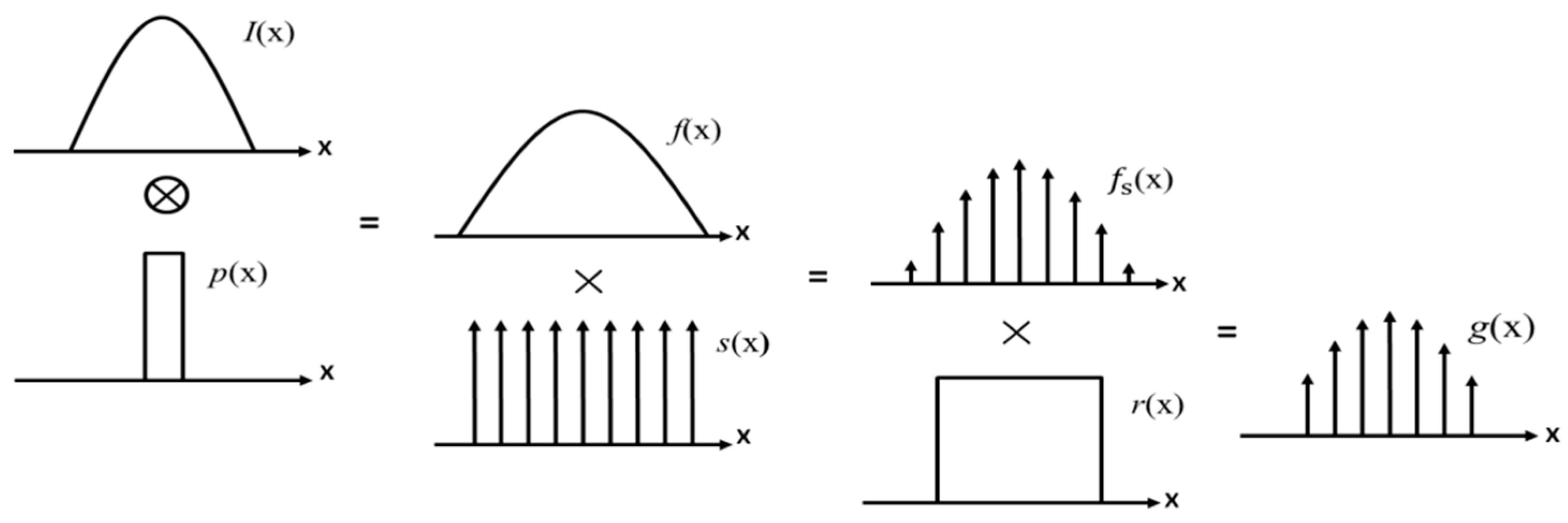
Figure 1. Decomposed graph of the star image sampling process.
Applsci 09 04751 g001
Figure 2. Simulated relationship between the systematic error and the ideal centroid location under different Gaussian widths.
Applsci 09 04751 g002
Figure 3. A truncated pixel detected signal in the centroid estimation process. (a) Signal intensity profiles and pixel detected signal (line: signal intensity profile e(x), bar: pixel detected signal e(k)). (b) The three-pixel sampling window r(x). (c) The windowed pixel signal (dark bar: pixel detected signal in r(x), light bar: pixel detected signal outside r(x)).
Applsci 09 04751 g003
Figure 4. Signal intensity profiles and pixel detected signals under different Gaussian widths σ P S F and centroid positions x 0 (line: signal intensity profile, bar: pixel detected signal in three-pixel window, y axis: relative intensity). (a) σ P S F = 0.3, x 0 = 2.0; (b) σ P S F = 0.3, x 0 = 2.25; (c) σ P S F = 0.3, x 0 = 2.5; (d) σ P S F = 0.671, x 0 = 2.0; (e) σ P S F = 0.671, x 0 = 2.25; (f) σ P S F = 0.671, x 0 = 2.5.
Applsci 09 04751 g004
Figure 5. The relationship curve between σ x ^ g and x 0 . (a) Gaussian width σ P S F = 0.3. (b) Gaussian width σ P S F = 0.671.
Applsci 09 04751 g005
Figure 6. Structure of the extreme learning machine.
Applsci 09 04751 g006
Figure 7. The relationship curve between σ x ^ g and   x ^ g . (a) Gaussian width σ P S F = 0.3. (b) Gaussian width σ P S F = 0.671.
Applsci 09 04751 g007
Figure 8. The fitting performance of the extreme learning machine optimized by the bat algorithm (BA-ELM). (a) Gaussian width σ P S F = 0.3. (b) Gaussian width σ P S F = 0.671.
Applsci 09 04751 g008
Figure 9. The fitting error of the BA-ELM compensation method. (a) Gaussian width σ P S F = 0.3. (b) Gaussian width σ P S F = 0.671.
Applsci 09 04751 g009
Figure 10. Experiment results of random positions. (a1,a2) Gaussian width σ P S F = 0.3. (b1,b2) Gaussian width σ P S F = 0.671.
Applsci 09 04751 g010
Figure 11. The prediction error of the BA-ELM compensation method. (a) Gaussian width σ P S F = 0.3. (b) Gaussian width σ P S F = 0.671.
Applsci 09 04751 g011
Figure 12. A simulated star image ( σ P S F = 0.3).
Applsci 09 04751 g012
Figure 13. The simulated star image ( σ P S F = 0.671).
Applsci 09 04751 g013
Table 1. The star sensor configuration.
ParameterValue
Image plane dimension512 pixels × 512 pixels
Field of view (FOV)12° × 12°
Principle point (256 pixels, 256 pixels)
Pixel size15 mm × 15 mm
Magnitude threshold6.0 Mv
Table 2. The systematic error before and after compensation of the simulated star image with σ P S F = 0.3.
NumberIXXBCEXBCXACEXAC
151.243951.29780.053951.24391.2326 × 10−8
272.736672.68290.053772.73661.1070 × 10−7
3361.2308361.24830.0535361.23082.1059 × 10−8
455.875855.83770.038255.87587.8417 × 10−8
5199.6277199.58910.0386199.62771.8986 × 10−7
666.215466.26810.052766.21543.8834 × 10−8
769.290369.34240.052169.29034.5690 × 10−9
8430.3110430.36090.0499430.31102.9145 × 10−8
9108.1923108.24280.0505108.19231.5801 × 10−9
1043.298043.34930.051443.29801.9520 × 10−8
Table 3. The systematic error before and after compensation of the simulated star image with σ P S F = 0.671.
NumberIXXBCEXBCXACEXAC
1387.9959387.88970.1062387.99598.5532 × 10−8
285.221685.27410.052585.22161.0517 × 10−7
355.988255.88420.104055.98823.4377 × 10−8
4486.1995486.25680.0072486.19953.4220 × 10−8
5464.0505464.14390.0933464.05052.9580 × 10−9
6378.8036378.74570.0579378.80362.3147 × 10−8
7507.9022507.82120.0811507.90223.9890 × 10−9
8307.8156307.75500.0606307.81562.3306 × 10−8
9240.8466240.77900.0676240.84662.2531 × 10−7
1089.893589.81460.078989.89353.7056 × 10−8
Table 4. Comparison of the BA-ELM compensation method with other compensation methods.
MethodTraining TimeRMSEPrediction Error
BP549.8 ms3.6230 × 10−4 2.0 × 10⁻³
AC--1.8460 × 10⁻⁴ 5.0 × 10⁻⁴
ELM11.5 ms5.5251 × 10−6 4.0 × 10⁻⁵
LSSVR204.6 ms3.0387 × 10−5 6.0 × 10⁻⁵
BA-ELM50,400 ms2.4532 × 10−8 3.0 × 10⁻⁷