Abstract
Stock price prediction has always been an important application in time series predictions. Recently, deep neural networks have been employed extensively for financial time series tasks. The network typically requires a large amount of training samples to achieve high accuracy. However, in the stock market, the number of data points collected on a daily basis is limited in one year, which leads to insufficient training samples and accordingly results in an overfitting problem. Moreover, predicting stock price movement is affected by various factors in the stock market. Therefore, choosing appropriate input features for prediction models should be taken into account. To address these problems, this paper proposes a novel framework, named deep transfer with related stock information (DTRSI), which takes advantage of a deep neural network and transfer learning. First, a base model using long short-term memory (LSTM) cells is pre-trained based on a large amount of data, which are obtained from a number of different stocks, to optimize initial training parameters. Second, the base model is fine-tuned by using a small amount data from a target stock and different types of input features (constructed based on the relationship between stocks) in order to enhance performance. Experiments are conducted with data from top-five companies in the Korean market and the United States (US) market from 2012 to 2018 in terms of the highest market capitalization. Experimental results demonstrate the effectiveness of transfer learning and using stock relationship information in helping to improve model performance, and the proposed approach shows remarkable performance (compared to other baselines) in terms of prediction accuracy.
1. Introduction
Forecasting stock prices has been a challenging problem, and it has attracted many researchers in the areas of economic market financial analysis and computer science. Accurate forecasts of the direction of stock price movement help investors make decisions in buying and selling stocks, and reducing unexpected risks. However, financial time series data are not only noisy and non-stationary in nature, but they are also easily affected by many factors, such as news, competitors, and natural factors [1]. Therefore, accurately predicting a stock price is highly difficult.
There are several stock market prediction models based on statistical analysis of data and machine learning techniques. The earliest studies tended to employ statistical methods, but these approaches did not perform well, and had limitations when applied to real-world stock data [2]. Recently, various machine learning algorithms, such as artificial neural networks (ANNs) [3], support vector machines (SVMs) [4], and random forests (RFs) [5], have been widely used in financial time series prediction tasks because these approaches can effectively learn the non-linear relationships between historical signals and future stock prices.
Over the past few decades, recurrent neural networks (RNNs) [6,7] have been used particularly for time series prediction because this type of network includes states that can capture historical information from an arbitrarily long context window. In our study, we use long short-term memory (LSTM) cells for sequence learning of financial market predictions. LSTM is a part of RNNs, and using LSTM cells can alleviate the problem of vanishing (and exploding) gradients [8]. However, in order to train LSTM cells effectively, the overfitting problem from an insufficient number of training samples should be considered [9]. Particularly, in stock price prediction, the number of data points that we can collect on a daily basis is only about 240 in a year. That is not sufficient, considering the number of model parameters. Currently, several methods have been found to avoid the overfitting problem, such as regularization techniques (i.e., L1 and L2 regularization [10]), dropout [11], data augmentation [12], and early stopping [13].
In recent years, transfer learning has been popularly used in training deep neural networks (DNNs) owing to the effectiveness of this technique in helping to reduce training time and to enhance prediction accuracy, despite a small amount of training data [14,15,16,17,18,19]. However, transfer learning has not been used much in time series prediction tasks. In this paper, we propose a framework called deep transfer with related stock information (DTRSI) to predict stock price movement, to mitigate the overfitting problem caused by an insufficient number of training samples, and to improve prediction performance by using the relationships between stocks. Specifically, our framework has two phases. First, a base model using LSTM cells is pre-trained with a large amount of data (which were obtained from a number of different stocks) to optimize initial training parameters. Secondly, the base model is fine-tuned with a small amount of the target stock data to predict the target stock’s price movement. The fine-tuned model is called a prediction model. For convenience, the target stock is called the company of interest (COI) stock. In addition, the prediction model is trained by using the different sets of input features that are constructed based on information about stocks related to the COI stock. In detail, we first calculate a one-day return, which shows the change of a stock’s closing price between two consecutive days. The first set of input features includes only one-day returns of the COI stock. The second set is the combination of one-day returns of COI stock and the index (e.g., Korea Composite Stock Price Index 200 (KOSPI 200) and Standard&Poor’s 500 (S&P 500)). The third set is the combination of one-day returns of the COI stock, the index, and stocks related to the COI stock (i.e., the highest cosine similarity to the COI stock, similar field to the COI, and the highest market capitalization).
In this study, to validate the proposed framework, as COI stocks, we choose top-five companies on the KOSPI 200 and top-five companies from five popular sectors in the S&P 500 in terms of market capitalization. The KOSPI 200 represents the benchmark indicator of the Korean capital market, and the S&P 500 is a globally important benchmark indicator for the United States (US) market.
The main contributions of our work can be summarized as follows:
- First, our work considers the overfitting problem caused by an insufficient amount of data in forecasting stock price movements. To address this challenge, a deep transfer-based framework is proposed in which transfer learning is used to effectively train the prediction model using only a small amount of COI stock data.
- Second, to enhance the prediction model performance, various types of input features are designed. The objective is to find suitable input features that may affect the quality and performance of a classifier. In our work, for a given COI stock, stocks that have relationships with the COI stock are first selected, and then, model inputs are formed based on features of the COI stock, the index (i.e., the KOSPI 200 or the S&P 500), and selected stocks. Three relationships are proposed: the highest cosine similarity (CS), similar field (SF), and the highest market capitalization (HMC). Specifically, CS selects stocks that have a direction in closing price movement that is most similar to the COI stock; SF finds stocks that have similar industrial products to the COI, even though there may be no direct closing price movement correlation between them; and HMC aims at choosing the largest companies in each stock market. The companies that are selected based on HMC may affect the COI’s closing price movements. Moreover, model inputs formed based on features of the COI stock and the index are called CI.
- Third, various experiments are conducted to validate our framework’s performance. Results show that the proposed approach outperforms four baselines: RF, SVM, K-nearest neighbors (KNN), and a recent model that used LSTM cells [20]. Specifically, our approach achieves a 60.70% average accuracy, compared to a 51.49% average accuracy from RF, a 51.57% average accuracy from SVM, a 51.77% average accuracy from KNN, and a 57.36% average accuracy from the existing model. Moreover, the performance of the SF selection method substantially dominates other considered methods in terms of average prediction accuracy. In addition, the number of similar-field companies in the input features can affect the prediction performance dramatically.
The rest of this paper is organized as follows: Section 2 summarizes the existing literature related to stock price prediction. Preliminaries, including base knowledge about long short-term memory and transfer learning, are presented in Section 3. Then, Section 4 and Section 5 describe dataset and preprocessing and our proposed framework, respectively. In Section 6, we analyze the evaluation results of the proposed model with different types of input, and we compare the performance of our approach with other benchmark models. Finally, the conclusions from this work are drawn in Section 7.
2. Related Works
2.1. Stock Market Prediction
Several studies have attempted financial time series predictions. Specifically, most early studies tended to employ statistical methods, such as the weighted moving average (WMA) [21], the generalized autoregressive conditional heteroskedasticity (GARCH) model [22], and the autoregressive integrated moving average (ARIMA) [23]. However, these approaches made many statistical assumptions, such as linearity and normality, whereas the financial time series is non-linear. Therefore, these approaches are not suitable for forecasting a stock price. Apart from the statistical models, machine learning techniques have been extensively applied to financial time series prediction tasks due to their capability in nonlinear mapping and generalization [3,4,24,25,26,27]. For instance, Adebiyi et al. [25] presented the performance of a multi-layer perceptron (MLP) model and compared it to the performance of an ARIMA model in forecasting stock prices on the New York Stock Exchange (NYSE). They concluded that the MLP model performed better than the ARIMA model in terms of the mean squared error (MSE). Kara et al. [27] used MLP and SVM to predict the direction of movement in the daily Istanbul Stock Exchange (ISE) National 100 Index. Experimental results indicated that their models outperformed the ordinary least square (OLS) regression model in terms of prediction accuracy. Although MLP can be used in financial time series prediction, several studies showed that MLP has some limitations in learning the patterns, as stock data have tremendous amounts of noise, and a high dimension. MLP often exhibits inconsistent and unpredictable performance on noisy data [28,29].
In recent years, with the significant advances in deep learning techniques, recurrent neural networks have emerged as a promising model for handling sequential data in various tasks such as natural language processing, speech recognition, and computer vision. Moreover, several studies proved that RNN including LSTM cells is the most useful model in the financial time series prediction problem [30,31,32,33,34,35,36]. For example, Chen et al. [30] introduced a stock price movement prediction model based on LSTM. A lot of basic variables for stocks (e.g., high price, low price, closing price, volume, and adjusted closing price) are considered as input features. The model was trained on samples and tested using another samples. They concluded that LSTM could attain satisfactory performance in predicting China’s index price movements. Chung and Shin [34] employed an LSTM network to predict KOSPI index prices in the next day. They tested their method on KOSPI index data from 2000 to 2016 and found that the method achieved satisfactory performance. In [33], the authors integrated wavelet transforms (WTs) and recurrent neural network based on an artificial bee colony algorithm. The closing price values of the Dow Jones Industrial Average Index (DJIA), the London FTSE-100 Index (FTSE), Tokyo Nikkei-225 Index (Nikkei), and Taiwan Stock Exchange Capitalization Weighted Stock Index (TAIEX) were predicted. Results showed that their proposed approaches can maximize profits. Bao et al. [35] employed a denoising approach using WTs as data-preprocessing, and then applied stack autoencoders (SAEs) to extract deep daily features. Their proposed framework outperformed their baseline methods in terms of MSE. However, most of the previous studies aimed at finding a suitable framework that can learn from non-linear and noisy stock data based on assumptions about sufficient data, whereas, in fact, collecting more stock data is difficult with only about 240 data points available in a year. Meanwhile, our work aims at finding a novel approach that can effectively train an LSTM network despite having an insufficient amount of data.
2.2. Feature Selection for Stock Price Prediction
Stock prices are dramatically affected by many factors [1]. Some basic factors (financial ratios, technical indicators, macroeconomic indices, and competitors) should be used as important factors affecting the rise and fall in stock values. However, each researcher has chosen their input features differently for their prediction models [37]. In the following subsection, choosing input features for stock price movement prediction in recent studies is presented.
Several studies have used technical indicators (TIs) as input variables in forecasting future stock prices [26,38,39,40,41,42,43]. For example, for every day of training, to construct input feature vectors, the authors in [40,42] calculated 10 technical indicators (e.g., simple moving average, exponential moving average, and relative strength index) from raw time series data including opening price, closing price, high and low prices, and trading volume. Thus, they fed these technical indicator values into their models (based on SVM, ANN, and RF). Experimental results showed satisfactory prediction accuracy. Although technical indicators have been used widely in stock market prediction tasks, the selection of suitable indicators to form model inputs from among various technical indicators is still a challenging task.
Other studies were aimed at predicting stock prices given textual information from the financial news [44,45,46]. For instance, Akita et al. [44] converted newspaper articles into distributed representations via paragraph vectors and modeled the temporal effects of past events with an LSTM on predicting opening prices of stocks on the Tokyo Stock Exchange. Bollen et al. [47] revealed that investor’s emotions derived from Twitter have impacts on stock indicators. Michael et al. [48] first introduced a novel word representation method to extract important features from text data. Then, they used an SVM model to predict the direction of stock price movements in the next day. Those studies proved that textual information can be used in financial time series prediction tasks. However, their objective was to find effective feature extraction methods to help improve prediction performance. Moreover, most of the research assumed that a company’s news was always published each day, which is a rare case in reality.
Fischer and Krauss [20] deployed an LSTM network in predicting the directional movement of constituent stocks of the S&P 500 from 1992 to 2015. In their research, they used 240 one-day returns as input variables for the prediction model. They divided the entire time period into 23 study periods, where each study period had 750 days (approximately three years). Their model was compared with other classifier models, such as RF, DNN, and logistic regression. They provided an in-depth guide on data preprocessing, as well as the development of LSTM for financial time series prediction tasks, and concluded that their approach outperformed other baselines over 23 study periods in terms of average prediction accuracy, shape ratio, and profit. However, in their study, they only used one-day returns of the target stock to form input models. In contrast, our work takes relationships between other stocks and the target stock into account in designing effective input. Thus, the proposed approach is compared to the work by Fischer and Krauss [20]. Results show that the considered relationships can enhance the performance of the prediction model.
3. Preliminaries
3.1. Long Short Term Memory
Long short-term memory (LSTM) is a specific recurrent neural network (RNN) architecture. It can learn temporal patterns from sequential data, and overcomes the vanishing gradient problem in a standard RNN [8]. Moreover, LSTMs have gating mechanisms to regulate the flow of information. The amount of information that will be retained is systemically determined at each time step. Therefore, LSTMs can memorize temporal patterns over a long time series. The architecture of an LSTM cell is illustrated in Figure 1, in which , , and are defined as the input, the hidden state, and the cell state, respectively, at time t. An LSTM cell has three gates: , , and , which are called the forget gate, the input gate, and the output gate, respectively. Note that ⊗ is point-wise multiplication. and activation functions are marked as and , respectively. Here, the activation function is defined as . The function is used in order to update the hidden state. Moreover, the activation function is defined as . The function helps form the output value in the range of . If the output is close to 0, most information is lost. If the output value is close to 1, it means that more information is allowed.
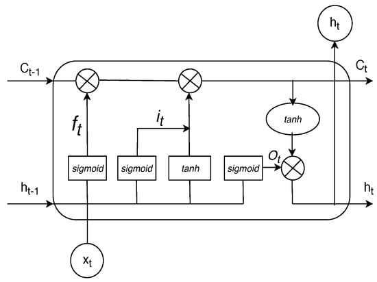
Figure 1.
The structure of long short-term memory (LSTM) block.
The calculations for the forget gate (), the input gate (), the output gate (), the cell state () and the hidden state () are performed using the following formulas:
where , , , , , , , and are weight matrices, and , , , and are bias vectors.
3.2. Transfer Learning
Transfer learning is a type of machine learning technique. Here, transfer learning aims at extracting the knowledge from one or more source tasks, and applies the knowledge to a target task. The key to transfer learning is achieving a remarkable improvement in performance by learning from similar tasks. In addition, it can avoid “starting from scratch” when training on an individual task, and can reduce the training time. Therefore, we can achieve better performance and reduce training time by using a small number of training samples for a new task. Due to this advantage, in our study, we use transfer learning to overcome the limited-data problem. We obtain a large source data and learn knowledge from them before transferring the knowledge into the target data (i.e., where data from only the target stock are used). A large source of data can be formed by mixing other stock data, and Section 5 will discuss this in detail.
According to the availability of labels in the source dataset and the target dataset, transfer learning approaches are divided into three categories: inductive transfer learning, transductive transfer learning, and unsupervised transfer learning [49]. Table 1 shows the differences between these categories in transfer learning.

Table 1.
Different settings of transfer learning.
In our case, inductive transfer learning is applied because labeled data in both the source data and the target data are available. Moreover, in this study, we first obtained a large source data from a large number of different stocks. Then, a base deep neural network was trained with obtained source data, and we attained a well-trained deep network based on validation performance. In the next step, a prediction model was constructed that has the same architecture as the base model. Thus, we transferred the trained parameters of the base model including weights and biases to initialize the prediction model. Finally, the prediction model was fine-tuned by using a small amount of target data and we optimized these parameters to achieve final prediction performance. Therefore, among the different approaches for inductive transfer learning setting (i.e., instance-transfer, feature-representation-transfer, parameter-transfer, and relational-knowledge-transfer) [49], parameter-transfer was chosen for our approach.
4. Dataset and Preprocessing
For our experiments, we use historical closing price data from two stock market indices, i.e., the KOSPI 200 and the S&P 500, and included all stocks in each index from 31 July 2012 to 31 July 2018 on a working-day basis. These data were obtained from the Yahoo financial website (https://finance.yahoo.com/). Let n denote the number of stocks we collected.
During the entire time period from 2012 to 2018, this study considered three sub-study periods, as shown in Figure 2.
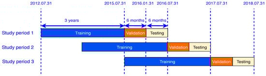
Figure 2.
Study periods.
Each study period included stock data from four years, which were partitioned into three parts: the first three years for the training set, next six months for the validation set, and final six months for the test set.
Let denote the closing price of stock s on day t. In our context, corresponds to the position of stocks in descending order of market capitalization. Similar to [20], we define as the return of stock s on day t over the previous p days (i.e., the difference in closing price between day t and day ) as follows:
For all stock data, we first calculate one-day () returns, , for each day t of each stock s. Then, 20 one-day returns of the most recent 20 days with day are stacked into one feature vector, , on day t. In total, in each study period, the numbers of samples for the training set, the validation set, and the testing set of each stock are described in Table 2.
Table 2.
Specification of the number of samples for each set.
Meanwhile, is used to indicate the output of the estimation model, which shows the change in the closing price of each stock s between two consecutive days (day t and day ). For example, indicates that an increase in the closing price on day , compared to the previous day, and means a decrease in the closing price.
5. Deep Transfer with Related Stock Information (DTRSI) Framework
In this section, the DTRSI framework is described. Figure 3a shows the specific procedures of the proposed framework. First, the source data are obtained from 50 different stocks. Then, a base model that has the architecture as shown in Figure 3b is trained by using the obtained source data. Note that FC is defined fully connected layers. In the next step, a prediction model is constructed that has the same architecture as the base model. Finally, the prediction model is fine-tuned by using a small amount of data from a COI stock and uses different types of input features (constructed based on stock relationships) to predict COI stock price movements.
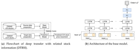
Figure 3.
The framework and the model architecture.
5.1. Base Model Construction
In this subsection, we describe how to train the base model, which consists of two steps. The first step is preparing a large source of data obtained from 50 available stocks. The second step is the training process. Each step is described below in more detail.
5.1.1. Source Data Preparation
In this study, three different source data with three different types of input features are employed. Specifically, Type I input features are only one-day returns of the COI stock, Type II input features are a combination of one-day returns of the COI stock and an index (e.g., KOSPI 200 and S&P 500), and Type III input features are a combination of one-day return values of the COI stock, the index and other stocks that have the highest cosine similarity to the COI stock.
Let denote an input that is used in predicting the closing price movement of stock s on day . In addition, , , and are feature vectors of stock s, the index, and related stocks with stock s, respectively, on day t, in which m is the number of stocks that are related to stock s. As defined in Section 4, , , and . In the base model, , , and represent the Type I input features, the Type II input features, and the Type III input features, respectively. Let and denote the number of training samples of source data and the number of training samples of each stock s, respectively.
In our work, three dimensional tensors (, , and ) with dimensions of corresponding to the source data of three types of input features, are constructed, where k is the number of input features. , and are illustrated in Figure 4, in which each matrix with dimensions of corresponds to one training sample.
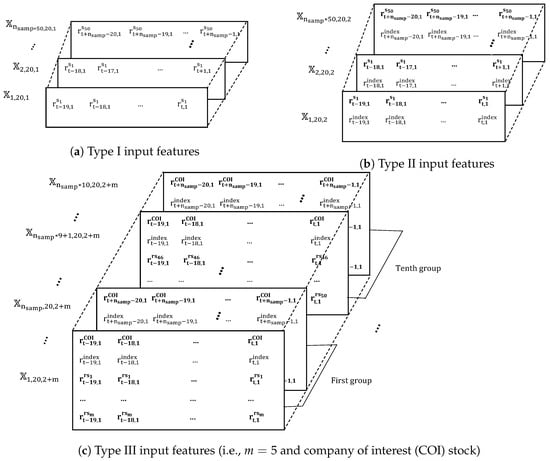
Figure 4.
Training samples with different types of input features.
Specifically, in the Type I input features and the Type II input features, we choose data from the top 50 stocks in terms of market capitalization, in which and stack them into one large dataset. In these cases, . For example, the number of training samples becomes approximately for the first study period. Note that for Type I input features and Type II input features, respectively. A main objective is to optimize model parameters by using training samples from 50 stocks instead of using training samples from only one stock.
Unlike the two first types of input features, in the Type III input features, we first choose 50 stocks closest (in terms of cosine similarity) to each COI stock, because features of these stocks may improve the base model performance. From , the 50 related stocks are randomly divided into groups, and each group includes m stocks. For instance, when , 10 different groups will be generated. An illustration is provided in Figure 4c, which shows how each group is used to design Type III input features. As shown in Figure 4c, for each COI stock, each , ,..., denotes the inputs designed from 10 generated groups. In the Type III input features, with each , training samples are fed into the base model to predict COI stock price movements. In our study, is taken into account. In this case, and . By considering these different groups, we bring two benefits to train the network. First, the number of training samples increases by . Second, more relevant and effective features can be used in constructing model inputs.
5.1.2. Training Process
For training the base model, a variety of network architectures which have a different number of layers, hidden units, and activation functions were examined. Then, from among the considered configurations, the most appropriate network architecture was selected based on the highest performance over the validation set. The topology of our LSTM model is as follows:
- The input layer has units that equal the number of features and 20 timesteps.
- There are two LSTM layers, which are followed by two fully connected layers (marked FC in Figure 3b). Each layer has 16 units and dropout regularization is applied to the outputs of each hidden layer in order to mitigate the overfitting problem. Keep probability values are set to .
- The output layer has one sigmoid activation unit.
Moreover, weight and bias values are initialized with the normal distribution. A learning rate in RMSprop optimization [50], the batch size, and the maximum training epochs are selected as , 512, and 5000, respectively.
5.2. Training the Prediction Model
In this subsection, we discuss how to train the prediction model. This model has the same architecture as the base model, and initial values of parameters are set to parameter values found for the base model. The prediction model takes data from only the COI stock for training task. Moreover, six different sets of input features (, , , , , and ) are considered, which are fed into the prediction model to predict COI stock price movement on day . Table 3 defines the notations that are used in this subsection.
Table 3.
Definitions of notations.
Each input vector is formed as follows:
In training the prediction model, six dimensional tensors, , , , , , and , with dimensions of are constructed as the training data for six types of input vectors, , , , , , and , respectively. Thus, we train six different prediction models using six different types of training data. Note that the base model and the prediction model have the same feature space. All training data of the prediction model are fed into the base model correspondingly, as shown in Table 4.
Table 4.
Specification of the training data fed to each model.
The learning rate and the maximum number of epochs are and 500, respectively. A small learning rate is chosen to avoid distorting pre-trained parameters too quickly.
6. Experimental Results
In this section, we present details on how we evaluate the performance of the proposed approach. Moreover, the influence of other information in predicting stock closing price movements based on the performance of different types of input features is also discussed in detail. To assess the performance of the prediction model, we use standard performance metrics (e.g., prediction accuracy). In this study, prediction accuracy is defined as the number of correctly classified outputs among the total number of outputs from the test data. In addition, our experiments are implemented by using keras (https://keras.io/) and scikit-learn (https://scikit-learn.org/stable/) libraries.
6.1. Effectiveness of Different Types of Input Features
In this subsection, the performance of our approach is examined using six different types of input features for the top five companies on the KOSPI 200 (i.e., Samsung Electronics Co. ( Suwon, Korea), SK Hynix Inc. (Icheon-si, Korea), Celltrion (Incheon, Korea), Hyundai Motor Co. (Seoul, Korea), and LG Chem (Seoul, Korea)) and the top five companies from five popular sectors on the S&P 500 (i.e., Apple Inc. (Cupertino, CA, USA), Amazon.com Inc. (Seattle, WA, USA), Boeing Company (Chicago, IL, USA), Johnson & Johnson (New Brunswick, NJ, USA), and JPMorgan Chase & Co. (New York, NY, USA)). Note that Table 5 uses COI, CI, CI+CS, CI+SF, CI+HMC, and CI+RND as the names of input features , , , , , and , respectively. Recall that CI is defined as model inputs formed based on features of the COI stock and the index; CS, SF, HMC, and RND are represented the relationship between other stocks and the COI stock such as the highest cosine similarity, similar field, the highest market capitalization, and randomly chosen, respectively.
Table 5.
Average accuracy of the different types of input variables over all study periods.
As seen in Table 5, the average prediction accuracy with CI+SF is the highest over all the study periods. Specifically, CI+SF obtains the highest average accuracy at 60.64%, compared to 53.74% and 56.35% for COI and CI, respectively. In addition, our model with CI+CS, CI+HMC and CI+RND achieves 58.91%, 58.59%, and 55.87%, respectively. This indicates that similar-field companies help to significantly improve the prediction accuracy of the model, compared to other considered factors.
Overall, the prediction model with CI+SF obtains the highest performance for almost all of the stocks. In particular, the prediction model with CI+SF effectively predicts Hyundai Motor Co. with a 64.54% average accuracy and Amazon.com Inc. with a 62.65% average accuracy over all study periods. However, in case of Apple Inc., CI attains 60.49% accuracy, which is slightly better than the 59.88% accuracy from CI+SF. One reason may be that Apple Inc. is the largest company in the United States and it is better coupled with the S&P 500.
In CI+SF, stocks from a similar field (e.g., similar industrial products) to the COI stock are selected. In fact, two companies in the same industry affect each other dramatically [44]. For example, an event like a “Samsung recall” may decrease Samsung’s stock value while increasing the stock price of SK Hynix Inc. at the same time because SK Hynix Inc. is the world’s second-largest memory chip-maker (after Samsung). In contrast, CI+CS uses stocks that have the most similar direction in closing price movements. In our work, cosine similarity between two vectors including one-day returns of two stocks is calculated over the entire training time period. As shown in Table 5, CI+SF achieves better average accuracy than CI+CS by 1.73%.
Additionally, CI+HMC aims at using top stocks that have the highest market capitalization in order to construct model inputs. When the COI is one of the top companies (e.g., Samsung Electronics Co., SK Hynix Inc, Apple Inc., or Amazon.com Inc.), CI+HMC obtains slightly better performance than CI+CS. Unlike these top companies, in the case of JPMorgan Chase & Co., CI+HMC achieves the worst performance at 54.01% average accuracy. Note that JPMorgan Chase & Co. is the largest company in the US financial field. Meanwhile, top companies of the US are companies working in the information technology field (e.g., Apple Inc., Alphabet Inc Class A (Mountain View, CA, USA), Microsoft Corp. (Redmond, WA, USA), and Facebook Inc. (Menlo Park, CA, USA)). Therefore, considering CI+HMC may not affect to JPMorgan Chase & Co.’s stock price movements, and may make irrelevant input features. As we can see in Table 5, in case of JPMorgan Chase & Co., CI+HMC obtains slightly lower performance than CI, which does not use information about other stocks.
Moreover, in our study, we train the prediction model with CI+RND. In this type of input, we choose other companies randomly (i.e., they may have no relationship to the COI stock). From the empirical results presented in Table 5, CI+RND provides lower performance than CI in terms of average prediction accuracy over all study periods. It proves that adding unnecessary information does not help improve the model’s performance.
One should note that CI+CS, CI+SF, and CI+HMC attain higher prediction accuracy than CI, and COI achieves the lowest performance. It indicates that by adding more relevant information, the performance of the prediction model is generally enhanced.
6.2. Effectiveness of the Proposed Approach versus Benchmark Models
In this subsection, we evaluate the performance of our model compared to four baseline classifiers, which are SVM, RF, KNN, and an existing model using LSTM cells [20]. First, the input vector for training four baseline models is constructed. Specifically, in constructing input vectors for the SVM, RF, and KNN models, five returns are stacked into one feature vector , which is used as an input vector. Unlike these models, in [20], they used 240 one-day returns, , to design input vectors, in which . Therefore, the input model is formed as . All returns, , are calculated by using Equation (6). In addition, targets of the baseline models are defined in the same way as the targets of our model in Section 4.
Two kinds of non-linear kernels (i.e., the radial basis function (RBF) kernel and the polynominal kernel) of SVM are considered. Hyperparameters of SVM (e.g., of RBF kernel, degree d of polynominal, and regularization C), hyperparameters of RF (e.g., the number of trees B, and maximum depth J), and hyperparameters of KNN (e.g., the number of neighbors K) are chosen by grid search for each branch. For choosing hyperparameters of the SVM model, the searching interval for , d, and C is with a step size of , with a step size of 1, and , respectively. The search range with a step size of 10 and range with a step size of 1 are considered for number of trees and maximum depth of RF model, respectively. Also, the search range with a step size of 1 is considered for number of neighbors of KNN model. The model from [20] consists of the input layer with one feature and 240 timesteps, one LSTM layer with hidden neurons and a dropout of , and the output layer with two neurons and softmax activation function.
As shown in Table 6, the performance of our proposed approach is the highest, with a 60.70% average accuracy in the study periods, while the SVM, RF, and KNN methods show low performance with 51.57%, 51.49%, and 51.77% average accuracy, respectively. Note that even when our approach uses only one-day returns of COI stock, it achieves 53.74% average accuracy, which is higher than SVM, RF, and KNN models by 2.17 percentage points, 2.25 percentage points, and 1.97 percentage points, respectively. It indicates that simple classifier models cannot extract input features effectively. Moreover, the overfitting problem may occur in training the SVM, RF, and KNN models due to the insufficient amount of data, whereas our approach based on transfer learning can reduce the influence of this problem.
Table 6.
Comparisonof our proposed approach and baselines over all study periods. Support vector machine (SVM), random forest (RF), K-nearest neighbors (KNN).
Compared to the existing model from [20], our approach improves the average accuracy by 3.34%. In [20], the model predicted COI stock price movement on day based on only one-day returns of the COI stock over one year. In fact, the direction of stock price movement is affected by other factors [1]. Unlike [20], related stocks are considered in our study. Results prove the effectiveness of using returns of related stocks to form the model input.
Overall, the proposed approach outperforms the model in [20] for all stocks, particularly, in the case of Hyundai Motor Co. company, with only 57.83% average accuracy from the existing model, compared to 64.54% average accuracy of our proposed approach (a broad difference of 6.71 percentage points). Additionally, 5.11% and 4.63% higher average accuracy are achieved for SK Hynix Inc and Amazon.com Inc., respectively. However, Table 6 illustrates similar average accuracy for the proposed approach and the existing model in predicting stock price movements of LG Chem, at 60.05% and 58.78%, respectively.
6.3. Performance Based on Different Numbers of Similar Companies
In this subsection, we concentrate on examining the influence of the number of stocks from a field similar to the COI stock when predicting stock price movement. The number of stocks varies: .
As shown in Table 7, the performance of predicting stock price movements of each company dramatically depends on the value of m. Specifically, displays the lowest performance at 55.93% average accuracy. However, with Hyundai Motor Co. and LG Chem, achieves remarkable performance at 64.22% and 56.87% average accuracy, respectively, compared to the others.
Table 7.
Average accuracy for different numbers of similar-field stocks over all study periods.
In addition, both and obtain similar performances at 57.97% and 57.62% average accuracy. In the Korean market, unlike Hyundai Motor Co. and LG Chem, the performance from stock price movement prediction for two companies (Samsung Electronics Co. and SK Hynix Inc) is the highest when . For instance, with Samsung Electronics Co., achieves 59.42% average accuracy, compared to 56.56% and 52.39% average accuracy when and , respectively. A similar trend is present in the US market, as shown in Table 7, particularly, for Apple Inc., with only 52.68% average predictive accuracy when , compared to 58.96% average accuracy when (a broad difference of 6.18 percentage points).
It should be highlighted that the value of m is considered as a hyperparameter of the prediction model and this value should be chosen carefully for each company.
7. Conclusions
In this paper, a novel framework called DTRSI is proposed to predict stock price movements by using an insufficient amount of data, yet with satisfactory performance. The framework takes full advantage of parameter transfer learning and a deep neural network. Moreover, we leverage relationships between stocks into constructing effective inputs to enhance the prediction model performance. Applied to the Korean stock market and the US stock market, experimental results show that the proposed approach performs better than other baselines (e.g., SVM, RF, KNN, and the model from [20]) in terms of average prediction accuracy. Moreover, stocks related to the COI stock are more useful in financial time series prediction tasks. Among the considered relationships, the prediction model using the returns of companies with a field similar to the COI achieved the highest performance.
To the best of our knowledge, this is the first study using a combination of transfer learning and long short-term memory in financial time series prediction tasks. Although the proposed integrated system has satisfactory prediction performance, it still has some drawbacks. First, our model has a large number of parameters by the nature of deep neural network. Therefore, the training process needs considerable time and computational resources, compared to other approaches. Second, finding a suitable number of stocks chosen in obtaining source data for the base model should be considered in order to enhance predictive accuracy. In addition, we use only the one-day returns of stocks, whereas market sentiment also helps make profitable models. In particular, several pre-trained models for the sentiment analysis task are being employed extensively. Therefore, our future task will be to design an optimized trading system that uses multiple types of source data, including numerical data (e.g., returns) and sentiment information.
Author Contributions
Conceptualization, S.Y. and T.-T.N.; methodology, T.-T.N. and S.Y.; software, T.-T.N.; validation, T.-T.N. and S.Y.; formal analysis, T.-T.N. and S.Y.; investigation, T.-T.N. and S.Y.; resources, S.Y.; data curation, T.-T.N.; writing—original draft preparation, T.-T.N. and S.Y.; writing—review and editing, T.-T.N. and S.Y.; visualization, T.-T.N. and S.Y.; supervision, S.Y.; project administration, S.Y.; funding acquisition, S.Y.
Funding
This research was funded by the 2019 Research Fund of University of Ulsan.
Conflicts of Interest
The authors declare no conflict of interest
References
- Abu-Mostafa, Y.S.; Atiya, A.F. Introduction to financial forecasting. Appl. Intell. 1996, 6, 205–213. [Google Scholar] [CrossRef]
- Kim, H.J.; Shin, K.S. A hybrid approach based on neural networks and genetic algorithms for detecting temporal patterns in stock markets. Appl. Soft Comput. 2007, 7, 569–576. [Google Scholar] [CrossRef]
- Guresen, E.; Kayakutlu, G.; Daim, T.U. Using artificial neural network models in stock market index prediction. Expert Syst. Appl. 2011, 38, 10389–10397. [Google Scholar] [CrossRef]
- Lin, Y.; Guo, H.; Hu, J. An SVM-based approach for stock market trend prediction. In Proceedings of the 2013 International Joint Conference on Neural Networks (IJCNN), Dallas, TX, USA, 4–9 August 2013; pp. 1–7. [Google Scholar]
- Booth, A.; Gerding, E.; McGroarty, F. Predicting equity market price impact with performance weighted ensembles of random forests. In Proceedings of the 2014 IEEE Conference on Computational Intelligence for Financial Engineering & Economics (CIFEr), London, UK, 27–28 March 2014; pp. 286–293. [Google Scholar]
- Lipton, Z.C.; Berkowitz, J.; Elkan, C. A critical review of recurrent neural networks for sequence learning. arXiv, 2015; arXiv:1506.00019. [Google Scholar]
- Liu, Y.; Guan, L.; Hou, C.; Han, H.; Liu, Z.; Sun, Y.; Zheng, M. Wind Power Short-Term Prediction Based on LSTM and Discrete Wavelet Transform. Appl. Sci. 2019, 9, 1108. [Google Scholar] [CrossRef]
- Hochreiter, S.; Schmidhuber, J. Long short-term memory. Neural Comput. 1997, 9, 1735–1780. [Google Scholar] [CrossRef]
- Lee, M.C. Using support vector machine with a hybrid feature selection method to the stock trend prediction. Expert Syst. Appl. 2009, 36, 10896–10904. [Google Scholar] [CrossRef]
- Ng, A.Y. Feature selection, L 1 vs. In L 2 regularization, and rotational invariance. In Proceedings of the Twenty-First International Conference on Machine Learning, Banff, AB, Canada, 4–8 July 2004; p. 78. [Google Scholar]
- Srivastava, N.; Hinton, G.; Krizhevsky, A.; Sutskever, I.; Salakhutdinov, R. Dropout: A simple way to prevent neural networks from overfitting. J. Mach. Learn. Res. 2014, 15, 1929–1958. [Google Scholar]
- Wong, S.C.; Gatt, A.; Stamatescu, V.; McDonnell, M.D. Understanding data augmentation for classification: when to warp? In Proceedings of the 2016 International Conference on Digital Image Computing: Techniques and Applications (DICTA), Gold Coast, Australia, 30 November–2 December 2016; pp. 1–6. [Google Scholar]
- Caruana, R.; Lawrence, S.; Giles, C.L. Overfitting in neural nets: Backpropagation, conjugate gradient, and early stopping. In Proceedings of the Advances in Neural Information Processing Systems, River Edge, NJ, USA, 21 November 2001; pp. 402–408. [Google Scholar]
- Norouzzadeh, M.S.; Nguyen, A.; Kosmala, M.; Swanson, A.; Palmer, M.S.; Packer, C.; Clune, J. Automatically identifying, counting, and describing wild animals in camera-trap images with deep learning. Proc. Natl. Acad. Sci. USA 2018, 115, E5716–E5725. [Google Scholar] [CrossRef]
- Kermany, D.S.; Goldbaum, M.; Cai, W.; Valentim, C.C.; Liang, H.; Baxter, S.L.; McKeown, A.; Yang, G.; Wu, X.; Yan, F.; et al. Identifying medical diagnoses and treatable diseases by image-based deep learning. Cell 2018, 172, 1122–1131. [Google Scholar] [CrossRef]
- Oliver, A.; Odena, A.; Raffel, C.A.; Cubuk, E.D.; Goodfellow, I. Realistic evaluation of deep semi-supervised learning algorithms. In Proceedings of the Advances in Neural Information Processing Systems, Palais des Congrès de Montréal, QC, Canada, 17 November 2018; pp. 3235–3246. [Google Scholar]
- Lee, J.; Park, J.; Kim, K.; Nam, J. Samplecnn: End-to-end deep convolutional neural networks using very small filters for music classification. Appl. Sci. 2018, 8, 150. [Google Scholar] [CrossRef]
- Izadpanahkakhk, M.; Razavi, S.; Taghipour-Gorjikolaie, M.; Zahiri, S.; Uncini, A. Deep region of interest and feature extraction models for palmprint verification using convolutional neural networks transfer learning. Appl. Sci. 2018, 8, 1210. [Google Scholar] [CrossRef]
- Zhang, L.; Wang, D.; Bao, C.; Wang, Y.; Xu, K. Large-Scale Whale-Call Classification by Transfer Learning on Multi-Scale Waveforms and Time-Frequency Features. Appl. Sci. 2019, 9, 1020. [Google Scholar] [CrossRef]
- Fischer, T.; Krauss, C. Deep learning with long short-term memory networks for financial market predictions. Eur. J. Oper. Res. 2018, 270, 654–669. [Google Scholar] [CrossRef]
- Ziegel, E.R. Analysis of Financial Time Series; Taylor & Francis: London, UK, 2002; Volume 8, p. 408. [Google Scholar]
- Gabriel, A.S. Evaluating the Forecasting Performance of GARCH Models. Evidence from Romania. Procedia Soc. Behav. Sci. 2012, 62, 1006–1010. [Google Scholar] [CrossRef]
- Ariyo, A.A.; Adewumi, A.O.; Ayo, C.K. Stock price prediction using the ARIMA model. In Proceedings of the 2014 UKSim-AMSS 16th International Conference on Computer Modelling and Simulation, Cambridge, UK, 26–28 March 2014; pp. 106–112. [Google Scholar]
- Di Persio, L.; Honchar, O. Artificial neural networks architectures for stock price prediction: Comparisons and applications. Int. J. Circ. Syst. Signal Process. 2016, 10, 403–413. [Google Scholar]
- Adebiyi, A.A.; Adewumi, A.O.; Ayo, C.K. Comparison of ARIMA and artificial neural networks models for stock price prediction. J. Appl. Math. 2014, 2014, 614342. [Google Scholar] [CrossRef]
- Chen, Y.; Hao, Y. A feature weighted support vector machine and K-nearest neighbor algorithm for stock market indices prediction. Expert Syst. Appl. 2017, 80, 340–355. [Google Scholar] [CrossRef]
- Kara, Y.; Boyacioglu, M.A.; Baykan, Ö.K. Predicting direction of stock price index movement using artificial neural networks and support vector machines: The sample of the Istanbul Stock Exchange. Expert Syst. Appl. 2011, 38, 5311–5319. [Google Scholar] [CrossRef]
- Qiu, M.; Song, Y. Predicting the direction of stock market index movement using an optimized artificial neural network model. PLoS ONE 2016, 11, e0155133. [Google Scholar] [CrossRef]
- Göçken, M.; Özçalıcı, M.; Boru, A.; Dosdoğru, A.T. Integrating metaheuristics and artificial neural networks for improved stock price prediction. Expert Syst. Appl. 2016, 44, 320–331. [Google Scholar] [CrossRef]
- Chen, K.; Zhou, Y.; Dai, F. A LSTM-based method for stock returns prediction: A case study of China stock market. In Proceedings of the 2015 IEEE International Conference on Big Data (Big Data), Santa Clara, CA, USA, 29 October–1 November 2015; pp. 2823–2824. [Google Scholar]
- Di Persio, L.; Honchar, O. Recurrent neural networks approach to the financial forecast of Google assets. Int. J. Math. Comput. Simul. 2017, 11, 7–13. [Google Scholar]
- Liu, S.; Liao, G.; Ding, Y. Stock transaction prediction modeling and analysis based on LSTM. In Proceedings of the 2018 13th IEEE Conference on Industrial Electronics and Applications (ICIEA), Wuhan, China, 31 May–2 June 2018; pp. 2787–2790. [Google Scholar]
- Hsieh, T.J.; Hsiao, H.F.; Yeh, W.C. Forecasting stock markets using wavelet transforms and recurrent neural networks: An integrated system based on artificial bee colony algorithm. Appl. Soft Comput. 2011, 11, 2510–2525. [Google Scholar] [CrossRef]
- Chung, H.; Shin, K.S. Genetic algorithm-optimized long short-term memory network for stock market prediction. Sustainability 2018, 10, 3765. [Google Scholar] [CrossRef]
- Bao, W.; Yue, J.; Rao, Y. A deep learning framework for financial time series using stacked autoencoders and long-short term memory. PLoS ONE 2017, 12, e0180944. [Google Scholar] [CrossRef]
- Ntakaris, A.; Mirone, G.; Kanniainen, J.; Gabbouj, M.; Iosifidis, A. Feature Engineering for Mid-Price Prediction With Deep Learning. IEEE Access 2019, 7, 82390–82412. [Google Scholar] [CrossRef]
- Atsalakis, G.S.; Valavanis, K.P. Surveying stock market forecasting techniques–Part II: Soft computing methods. Expert Syst. Appl. 2009, 36, 5932–5941. [Google Scholar] [CrossRef]
- Rodríguez-González, A.; García-Crespo, Á.; Colomo-Palacios, R.; Iglesias, F.G.; Gómez-Berbís, J.M. CAST: Using neural networks to improve trading systems based on technical analysis by means of the RSI financial indicator. Expert Syst. Appl. 2011, 38, 11489–11500. [Google Scholar] [CrossRef]
- Chen, Y.S.; Cheng, C.H.; Tsai, W.L. Modeling fitting-function-based fuzzy time series patterns for evolving stock index forecasting. Appl. Intell. 2014, 41, 327–347. [Google Scholar] [CrossRef]
- Patel, J.; Shah, S.; Thakkar, P.; Kotecha, K. Predicting stock and stock price index movement using trend deterministic data preparation and machine learning techniques. Expert Syst. Appl. 2015, 42, 259–268. [Google Scholar] [CrossRef]
- Chiang, W.C.; Enke, D.; Wu, T.; Wang, R. An adaptive stock index trading decision support system. Expert Syst. Appl. 2016, 59, 195–207. [Google Scholar] [CrossRef]
- Shynkevich, Y.; McGinnity, T.M.; Coleman, S.A.; Belatreche, A.; Li, Y. Forecasting price movements using technical indicators: Investigating the impact of varying input window length. Neurocomputing 2017, 264, 71–88. [Google Scholar] [CrossRef]
- Long, W.; Lu, Z.; Cui, L. Deep learning-based feature engineering for stock price movement prediction. Knowl.-Based Syst. 2019, 164, 163–173. [Google Scholar] [CrossRef]
- Akita, R.; Yoshihara, A.; Matsubara, T.; Uehara, K. Deep learning for stock prediction using numerical and textual information. In Proceedings of the 2016 IEEE/ACIS 15th International Conference on Computer and Information Science (ICIS), Okayama, Japan, 26–29 June 2016; pp. 1–6. [Google Scholar]
- Vargas, M.R.; De Lima, B.S.; Evsukoff, A.G. Deep learning for stock market prediction from financial news articles. In Proceedings of the 2017 IEEE International Conference on Computational Intelligence and Virtual Environments for Measurement Systems and Applications (CIVEMSA), Annecy, France, 26–28 June 2017; pp. 60–65. [Google Scholar]
- Yasir, M.; Durrani, M.Y.; Afzal, S.; Maqsood, M.; Aadil, F.; Mehmood, I.; Rho, S. An Intelligent Event-Sentiment-Based Daily Foreign Exchange Rate Forecasting System. Appl. Sci. 2019, 9, 2980. [Google Scholar] [CrossRef]
- Bollen, J.; Mao, H.; Zeng, X. Twitter mood predicts the stock market. J. Comput. Sci. 2011, 2, 1–8. [Google Scholar] [CrossRef]
- Hagenau, M.; Liebmann, M.; Neumann, D. Automated news reading: Stock price prediction based on financial news using context-capturing features. Decis. Support Syst. 2013, 55, 685–697. [Google Scholar] [CrossRef]
- Pan, S.J.; Yang, Q. A survey on transfer learning. IEEE Trans. Knowl. Data Eng. 2010, 22, 1345–1359. [Google Scholar] [CrossRef]
- Ruder, S. An overview of gradient descent optimization algorithms. arXiv, 2016; arXiv:1609.04747. [Google Scholar]


© 2019 by the authors. Licensee MDPI, Basel, Switzerland. This article is an open access article distributed under the terms and conditions of the Creative Commons Attribution (CC BY) license (http://creativecommons.org/licenses/by/4.0/).