Evaluation of Molecular Polarizability and of Intensity Carrying Modes Contributions in Circular Dichroism Spectroscopies

 ,
,  , , , and
Abstract
1. Introduction
2. Results
- (i)
- to simulate UV-Vis absorption spectra in the absence of vibronic effects:
- (ii)
- to simulate electronic CD (ECD) spectra [24]:and
- (iii)
3. Discussion
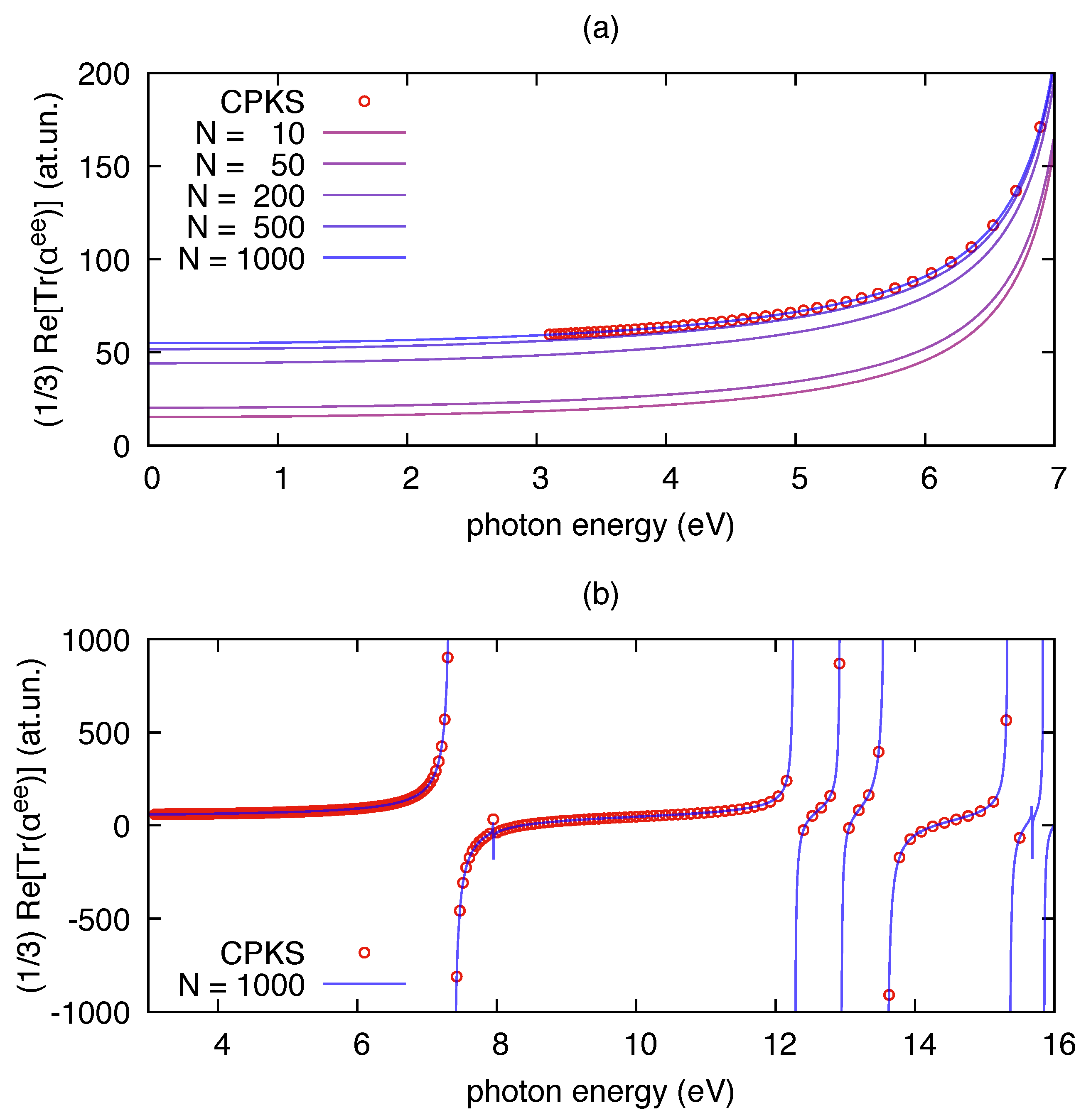
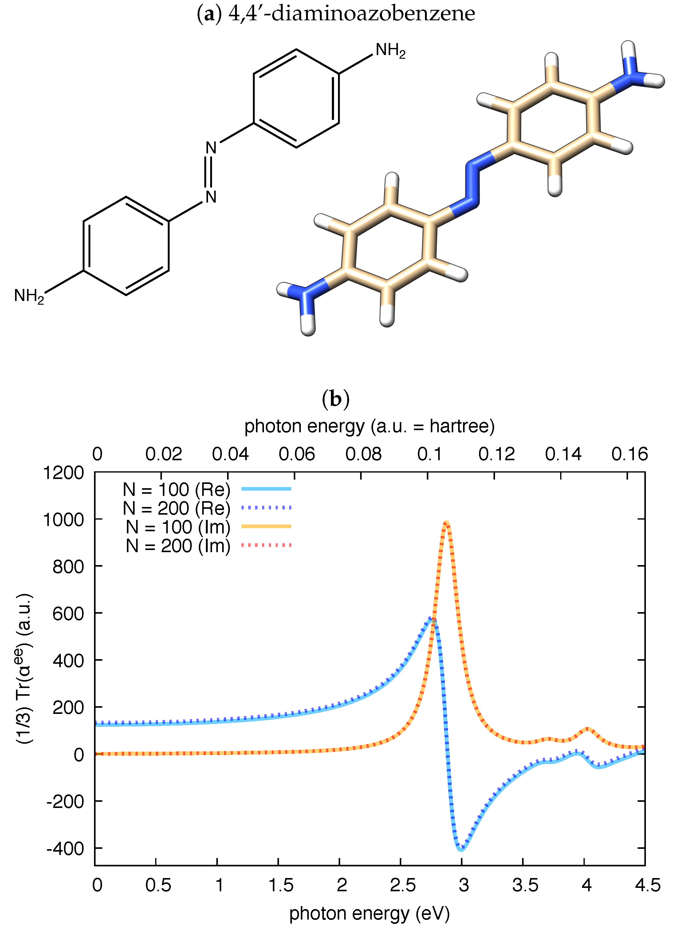
3.1. Polarizability Due to Electronic Transitions and UV-Vis Absorption
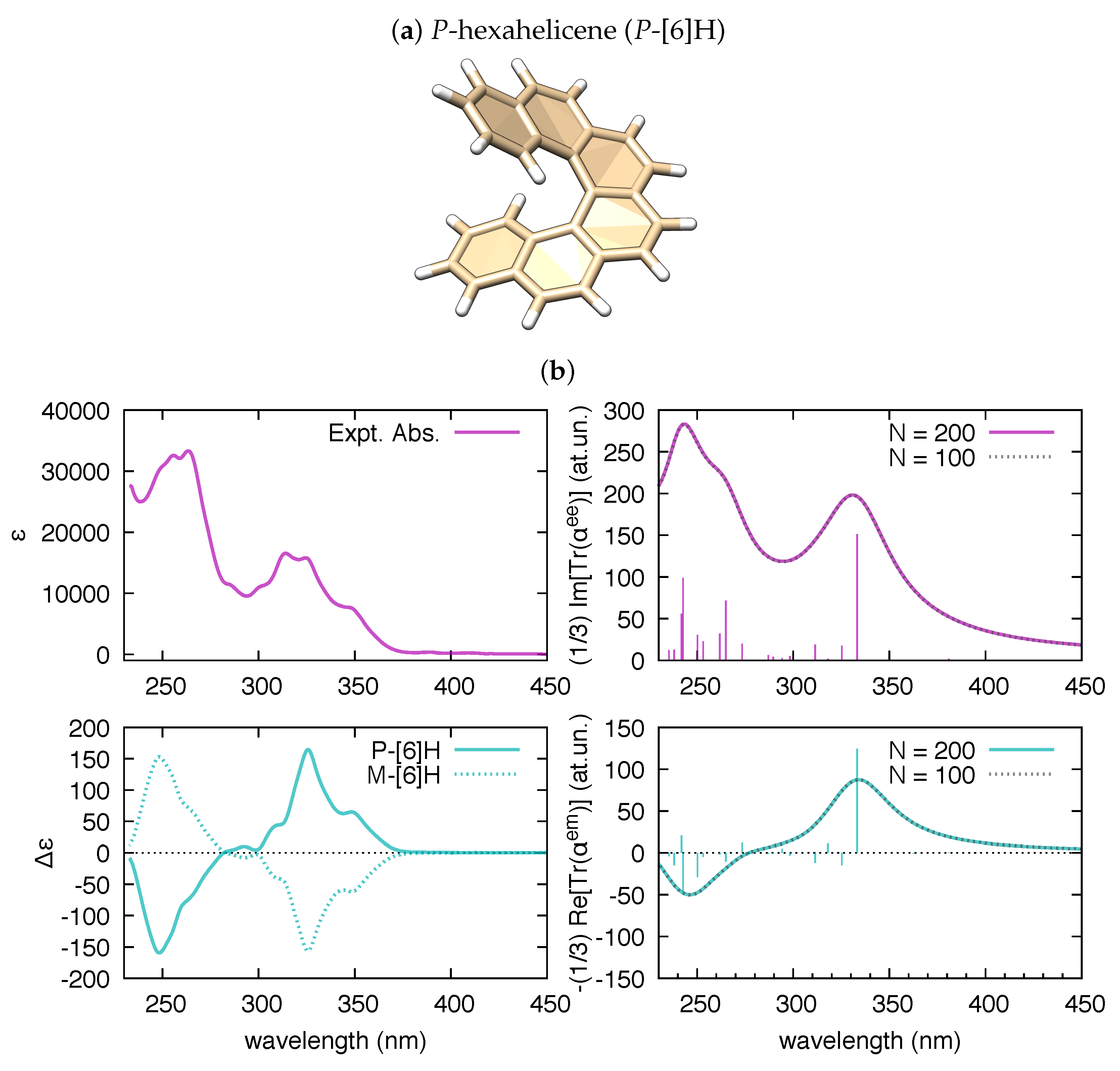
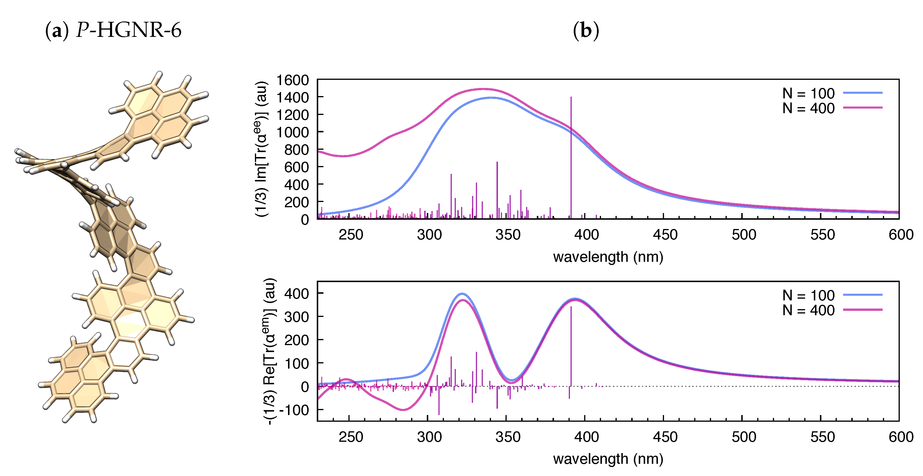
3.2. The Electric Dipole–Magnetic Dipole Polarizability and ECD
3.3. Vibrational Polarizabilities and IR/VCD Spectroscopies
3.4. Introducing Intensity-Carrying Modes in VCD
4. Materials and Methods
5. Conclusions
Author Contributions
Funding
Acknowledgments
Conflicts of Interest
Abbreviations
| AAT | Atomic Axial Tensor |
| APT | Atomic Polar Tensor |
| CD | circular dichroism |
| CPKS | coupled perturbed Kohn Sham equations |
| DFT | density functional theory |
| ECD | electronic circular dichroism |
| TDDFT | time-dependent density functional theory |
| VCD | vibrational circular dichroism |
Appendix A. Analysis of Polarizabilities in Resonance Condition
Appendix B. Polarizability as a Sum over Vibrational States
Appendix C. Relation with Lambert–Beer law
References
- Barone, V. Computational Strategies for Spectroscopy: From Small Molecules to Nano Systems; Wiley: Hoboken, NJ, USA, 2011. [Google Scholar]
- te Velde, G.; Bickelhaupt, F.M.; Baerends, E.J.; Fonseca Guerra, C.; van Gisbergen, S.J.A.; Snijders, J.G.; Ziegler, T. Chemistry with ADF. J. Comput. Chem. 2001, 22, 931–967. [Google Scholar] [CrossRef]
- TURBOMOLE V6.2 2010, a development of University of Karlsruhe and Forschungszentrum Karlsruhe GmbH, 1989-2007, TURBOMOLE GmbH, Since 2007. Available online: http://www.turbomole.org (accessed on 1 November 2019).
- Gordon, M.S.; Schmidt, M.W. Chapter 41—Advances in Electronic Structure Theory: GAMESS a Decade Later; Elsevier: Amsterdam, The Netherlands, 2005; pp. 1167–1189. [Google Scholar] [CrossRef]
- Frisch, M.J.; Trucks, G.W.; Schlegel, H.B.; Scuseria, G.E.; Robb, M.A.; Cheeseman, J.R.; Scalmani, G.; Barone, V.; Mennucci, B.; Petersson, G.A.; et al. Gaussian09 Revision D.01; Gaussian Inc.: Wallingford, CT, USA, 2009. [Google Scholar]
- Valiev, M.; Bylaska, E.J.; Govind, N.; Kowalski, K.; Straatsma, T.P.; Van Dam, H.J.J.; Wang, D.; Nieplocha, J.; Apra, E.; Windus, T.L.; et al. NWChem: A comprehensive and scalable open-source solution for large scale molecular simulations. Comput. Phys. Commun. 2010, 181, 1477–1489. [Google Scholar] [CrossRef]
- Aidas, K.; Angeli, C.; Bak, K.L.; Bakken, V.; Bast, R.; Boman, L.; Christiansen, O.; Cimiraglia, R.; Coriani, S.; Dahle, P.; et al. The Dalton quantum chemistry program system. Wiley Interdiscip. Rev. Comput. Mol. Sci. 2014, 4, 269–284. [Google Scholar] [CrossRef] [PubMed]
- Smith, D.G.A.; Burns, L.A.; Sirianni, D.A.; Nascimento, D.R.; Kumar, A.; James, A.M.; Schriber, J.B.; Zhang, T.; Zhang, B.; Abbott, A.S.; et al. Psi4NumPy: An Interactive Quantum Chemistry Programming Environment for Reference Implementations and Rapid Development. J. Chem. Theory Comput. 2018, 14, 3504–3511. [Google Scholar] [CrossRef]
- Neese, F. Software update: The ORCA program system, version 4.0. Wiley Interdiscip. Rev. Comput. Mol. Sci. 2018, 8, e1327. [Google Scholar] [CrossRef]
- Zerara, M. pyVib, a computer program for the analysis of infrared and Raman optical activity. J. Comput. Chem. 2008, 29, 306–311. [Google Scholar] [CrossRef]
- Bannwarth, C.; Grimme, S. A simplified time-dependent density functional theory approach for electronic ultraviolet and circular dichroism spectra of very large molecules. Comput. Theor. Chem. 2014, 1040–1041, 45–53. [Google Scholar] [CrossRef]
- Bannwarth, C.; Grimme, S. Electronic Circular Dichroism of Highly Conjugated π-Systems: Breakdown of the Tamm–Dancoff/Configuration Interaction Singles Approximation. J. Phys. Chem. A 2015, 119, 3653–3662. [Google Scholar] [CrossRef]
- Ren, S.; Caricato, M. Multi-state extrapolation of UV/Vis absorption spectra with QM/QM hybrid methods. J. Chem. Phys. 2016, 144, 184102. [Google Scholar] [CrossRef]
- Barone, V. The virtual multifrequency spectrometer: A new paradigm for spectroscopy. Wiley Interdiscip. Rev. Comput. Mol. Sci. 2016, 6, 86–110. [Google Scholar] [CrossRef]
- Fusè, M.; Egidi, F.; Bloino, J. Vibrational circular dichroism under the quantum magnifying glass: From the electronic flow to the spectroscopic observable. Phys. Chem. Chem. Phys. 2019, 21, 4224–4239. [Google Scholar] [CrossRef] [PubMed]
- Frediani, L.; Andreussi, O.; Kulik, H.J. Coding solvation: Challenges and opportunities. Int. J. Quantum Chem. 2019, 119, e25839. [Google Scholar] [CrossRef]
- Chiariello, M.G.; Raucci, U.; Coppola, F.; Rega, N. Unveiling anharmonic coupling by means of excited state ab initio dynamics: Application to diarylethene photoreactivity. Phys. Chem. Chem. Phys. 2019, 21, 3606–3614. [Google Scholar] [CrossRef] [PubMed]
- Galimberti, D.R.; Bougueroua, S.; Mahé, J.; Tommasini, M.; Rijs, A.M.; Gaigeot, M.P. Conformational assignment of gas phase peptides and their H-bonded complexes using far-IR/THz: IR-UV ion dip experiment, DFT-MD spectroscopy, and graph theory for mode assignment. Faraday Discuss. 2019, 217, 67–97. [Google Scholar] [CrossRef] [PubMed]
- Pezzotti, S.; Galimberti, D.R.; Gaigeot, M.P. Deconvolution of BIL-SFG and DL-SFG spectroscopic signals reveals order/disorder of water at the elusive aqueous silica interface. Phys. Chem. Chem. Phys. 2019, 21, 22188–22202. [Google Scholar] [CrossRef] [PubMed]
- Bloino, J.; Biczysko, M.; Barone, V. Anharmonic Effects on Vibrational Spectra Intensities: Infrared, Raman, Vibrational Circular Dichroism, and Raman Optical Activity. J. Phys. Chem. A 2015, 119, 11862–11874. [Google Scholar] [CrossRef] [PubMed]
- Micciarelli, M.; Conte, R.; Suarez, J.; Ceotto, M. Anharmonic vibrational eigenfunctions and infrared spectra from semiclassical molecular dynamics. J. Chem. Phys. 2018, 149, 64115. [Google Scholar] [CrossRef]
- Micciarelli, M.; Gabas, F.; Conte, R.; Ceotto, M. An effective semiclassical approach to IR spectroscopy. J. Chem. Phys. 2019, 150, 184113. [Google Scholar] [CrossRef]
- Zuehlsdorff, T.J.; Montoya-Castillo, A.; Napoli, J.A.; Markland, T.E.; Isborn, C.M. Optical spectra in the condensed phase: Capturing anharmonic and vibronic features using dynamic and static approaches. J. Chem. Phys. 2019, 151, 74111. [Google Scholar] [CrossRef]
- Schellman, J.A. Circular dichroism and optical rotation. Chem. Rev. 1975, 75, 323–331. [Google Scholar] [CrossRef]
- Kawiecki, R.W.; Devlin, F.; Stephens, P.J.; Amos, R.D.; Handy, N.C. Vibrational circular dichroism of propylene oxide. Chem. Phys. Lett. 1988, 145, 411–417. [Google Scholar] [CrossRef]
- Hu, L.; Huang, Y.; Pan, L.; Fang, Y. Analyzing intrinsic plasmonic chirality by tracking the interplay of electric and magnetic dipole modes. Sci. Rep. 2017, 7, 11151. [Google Scholar] [CrossRef] [PubMed]
- Mukamel, S.S. Principles of Nonlinear Optical Spectroscopy; Includes Index: New York, NY, USA; Oxford University Press: Oxford, UK, 1995. [Google Scholar]
- Toury, T.; Zyss, J.; Chernyak, V.; Mukamel, S. Collective Electronic Oscillators for Second-Order Polarizabilities of Push-Pull Carotenoids. J. Phys. Chem. A 2001, 105, 5692–5703. [Google Scholar] [CrossRef]
- Tretiak, S.; Mukamel, S. Density Matrix Analysis and Simulation of Electronic Excitations in Conjugated and Aggregated Molecules. Chem. Rev. 2002, 102, 3171–3212. [Google Scholar] [CrossRef] [PubMed]
- Kessler, J.; Bouř, P. Transfer of Frequency-Dependent Polarizabilities: A Tool To Simulate Absorption and Circular Dichroism Molecular Spectra. J. Chem. Theory Comput. 2015, 11, 2210–2220. [Google Scholar] [CrossRef] [PubMed]
- Moscowitz, A. Theoretical Aspects of Optical Activity Part One: Small Molecules. Adv. Chem. Phys. 1962, 4, 67–112. [Google Scholar] [CrossRef]
- Torii, H.; Ueno, Y.; Sakamoto, A.; Tasumi, M. Infrared Intensity-Carrying Modes and Electron-Vibration Interactions in the Radical Cations of Polycyclic Aromatic Hydrocarbons. J. Phys. Chem. A 1999, 103, 5557–5566. [Google Scholar] [CrossRef]
- Torii, H. Intensity-carrying modes important for vibrational polarizabilities and hyperpolarizabilities of molecules: Derivation from the algebraic properties of formulas and applications. J. Comput. Chem. 2002, 23, 997–1006. [Google Scholar] [CrossRef]
- Lee, K.S.H. Relations between electric and magnetic polarizabilities and other related quantities. Radio Sci. 1987, 22, 1235–1238. [Google Scholar] [CrossRef]
- Barron, L.D. Molecular Light Scattering and Optical Activity, 2nd ed.; Cambridge University Press: New York, NY, USA, 2009. [Google Scholar]
- Arrighini, G.P.; Maestro, M.; Moccia, R. Magnetic Properties of Polyatomic Molecules. I. Magnetic Susceptibility of H2O, NH3, CH4, H2O2. J. Chem. Phys. 1968, 49, 882–889. [Google Scholar] [CrossRef]
- Pelloni, S.; Lazzeretti, P. On the determination of the diagonal components of the optical activity tensor in chiral molecules. J. Chem. Phys. 2014, 140, 74105. [Google Scholar] [CrossRef] [PubMed]
- Ruud, K.; Helgaker, T. Optical rotation studied by density-functional and coupled-cluster methods. Chem. Phys. Lett. 2002, 352, 533–539. [Google Scholar] [CrossRef]
- Stephens, P.J.; Devlin, F.J.; Cheeseman, J.R.; Frisch, M.J. Calculation of Optical Rotation Using Density Functional Theory. J. Phys. Chem. A 2001, 105, 5356–5371. [Google Scholar] [CrossRef]
- Cheeseman, J.R.; Frisch, M.J.; Devlin, F.J.; Stephens, P.J. Hartree-Fock and Density Functional Theory ab Initio Calculation of Optical Rotation Using GIAOs: Basis Set Dependence. J. Phys. Chem. A 2000, 104, 1039–1046. [Google Scholar] [CrossRef]
- McWeeny, R. Natural Units in Atomic and Molecular Physics. Nature 1973, 243, 196. [Google Scholar] [CrossRef]
- Griffiths, D.J. Introduction to Electrodynamics, 4th ed.; Pearson: Boston, MA, USA, 2013; Re-Published by Cambridge University Press in 2017. [Google Scholar]
- Buckingham, A.D.; Fischer, P. Phenomenological damping in optical response tensors. Phys. Rev. A 2000, 61, 035801. [Google Scholar] [CrossRef]
- Mukamel, S. Causal versus noncausal description of nonlinear wave mixing: Resolving the damping-sign controversy. Phys. Rev. A 2007, 76, 021803. [Google Scholar] [CrossRef]
- Bialynicki-Birula, I.; Sowiński, T. Quantum electrodynamics of qubits. Phys. Rev. A 2007, 76, 062106. [Google Scholar] [CrossRef]
- Buckingham, A.D.; Fowler, P.W.; Galwas, P.A. Velocity-dependent property surfaces and the theory of vibrational circular dichroism. Chem. Phys. 1987, 112, 1–14. [Google Scholar] [CrossRef]
- Buckingham, A.D. Introductory lecture. The theoretical background to vibrational optical activity. Faraday Discuss. 1994, 99, 1–12. [Google Scholar] [CrossRef]
- Wilson, E.B.; Decius, J.C.; Cross, P.C. Molecular Vibrations: The Theory of Infrared and Raman Vibrational Spectra; Dover Books on Chemistry; Dover Publ.: New York, NY, USA, 1980. [Google Scholar]
- Stephens, P.J. Theory of vibrational circular dichroism. J. Phys. Chem. 1985, 89, 748–752. [Google Scholar] [CrossRef]
- Stephens, P.J. Gauge dependence of vibrational magnetic dipole transition moments and rotational strengths. J. Phys. Chem. 1987, 91, 1712–1715. [Google Scholar] [CrossRef]
- Nicu, V.P.; Neugebauer, J.; Wolff, S.K.; Baerends, E.J. A vibrational circular dichroism implementation within a Slater-type-orbital based density functional framework and its application to hexa- and hepta-helicenes. Theor. Chem. Acc. 2008, 119, 245–263. [Google Scholar] [CrossRef]
- Politzer, P.; Jin, P.; Murray, J.S. Atomic polarizability, volume and ionization energy. J. Chem. Phys. 2002, 117, 8197–8202. [Google Scholar] [CrossRef]
- Brinck, T.; Murray, J.S.; Politzer, P. Polarizability and volume. J. Chem. Phys. 1993, 98, 4305–4306. [Google Scholar] [CrossRef]
- Haghdani, S.; Davari, N.; Sandnes, R.; Åstrand, P.O. Complex Frequency-Dependent Polarizability through the π→π* Excitation Energy of Azobenzene Molecules by a Combined Charge-Transfer and Point-Dipole Interaction Model. J. Phys. Chem. A 2014, 118, 11282–11292. [Google Scholar] [CrossRef]
- Gingras, M. One hundred years of helicene chemistry. Part 3: Applications and properties of carbohelicenes. Chem. Soc. Rev. 2013, 42, 1051–1095. [Google Scholar] [CrossRef]
- Bürgi, T.; Urakawa, A.; Behzadi, B.; Ernst, K.H.; Baiker, A. The absolute configuration of heptahelicene: A VCD spectroscopy study. New J. Chem. 2004, 28, 332–334. [Google Scholar] [CrossRef]
- Abbate, S.; Lebon, F.; Longhi, G.; Fontana, F.; Caronna, T.; Lightner, D.A. Experimental and calculated vibrational and electronic circular dichroism spectra of 2-Br-hexahelicene. Phys. Chem. Chem. Phys. 2009, 11, 9039–9043. [Google Scholar] [CrossRef]
- Nakai, Y.; Mori, T.; Inoue, Y. Theoretical and Experimental Studies on Circular Dichroism of Carbo[n]helicenes. J. Phys. Chem. A 2012, 116, 7372–7385. [Google Scholar] [CrossRef]
- Johannessen, C.; Blanch, E.; Villani, C.; Abbate, S.; Longhi, G.; Agarwal, N.; Tommasini, M.; Lightner, D. Raman and ROA spectra of (-)- and (+)-2-Br-Hexahelicene: Experimental and DFT studies of a π-conjugated chiral system. J. Phys. Chem. B 2013, 117. [Google Scholar] [CrossRef] [PubMed]
- Abbate, S.; Longhi, G.; Lebon, F.; Castiglioni, E.; Superchi, S.; Pisani, L.; Fontana, F.; Torricelli, F.; Caronna, T.; Villani, C.; et al. Helical sense-responsive and substituent-sensitive features in vibrational and electronic circular dichroism, in circularly polarized luminescence, and in Raman spectra of some simple optically active hexahelicenes. J. Phys. Chem. C 2014, 118, 1682–1695. [Google Scholar] [CrossRef]
- Zanchi, C.; Lucotti, A.; Cancogni, D.; Fontana, F.; Trusso, S.; Ossi, P.; Tommasini, M. Functionalization of nanostructured gold substrates with chiral chromophores for SERS applications: The case of 5-Aza[5]helicene. Chirality 2018, 30, 875–882. [Google Scholar] [CrossRef] [PubMed]
- Daigle, M.; Miao, D.; Lucotti, A.; Tommasini, M.; Morin, J.F. Helically Coiled Graphene Nanoribbons. Angew. Chem. Int. Ed. 2017, 56, 6213–6217. [Google Scholar] [CrossRef] [PubMed]
- Manolopoulos, D.E. Proposal of a chiral structure for the fullerene C76. J. Chem. Soc. Faraday Trans. 1991, 87, 2861–2862. [Google Scholar] [CrossRef]
- Diederich, F.; Ettl, R.; Rubin, Y.; Whetten, R.L.; Beck, R.; Alvarez, M.; Anz, S.; Sensharma, D.; Wudl, F.; Khemani, K.C.; et al. The Higher Fullerenes: Isolation and Characterization of C76, C84, C90, C94, and C70O, an Oxide of D5h-C70. Science 1991, 252, 548–551. [Google Scholar] [CrossRef]
- Ettl, R.; Chao, I.; Diederich, F.; Whetten, R.L. Isolation of C76, a chiral (D2) allotrope of carbon. Nature 1991, 353, 149. [Google Scholar] [CrossRef]
- Orlandi, G.; Poggi, G.; Zerbetto, F. The circular dichroism spectrum of C76. A quantum chemical study. Chem. Phys. Lett. 1994, 224, 113–117. [Google Scholar] [CrossRef]
- Goto, H.; Harada, N.; Crassous, J.; Diederich, F. Absolute configuration of chiral fullerenes and covalent derivatives from their calculated circular dichroism spectra. J. Chem. Soc. Perkin Trans. 2 1998, 8, 1719–1724. [Google Scholar] [CrossRef]
- Kessinger, R.; Crassous, J.; Herrmann, A.; Rüttimann, M.; Echegoyen, L.; Diederich, F. Preparation of Enantiomerically Pure C76 with a General Electrochemical Method for the Removal of Di(alkoxycarbonyl)methano Bridges from Methanofullerenes: The Retro-Bingel Reaction. Angew. Chem. Int. Ed. 1998, 37, 1919–1922. [Google Scholar] [CrossRef]
- Furche, F.; Ahlrichs, R. Absolute Configuration of D2-Symmetric Fullerene C84. J. Am. Chem. Soc. 2002, 124, 3804–3805. [Google Scholar] [CrossRef] [PubMed]
- Bishop, D.M.; Gu, F.L.; Cybulski, S.M. Static and dynamic polarizabilities and first hyperpolarizabilities for CH4, CF4, and CCl4. J. Chem. Phys. 1998, 109, 8407–8415. [Google Scholar] [CrossRef]
- Gussoni, M.; Rui, M.; Zerbi, G. Electronic and relaxation contribution to linear molecular polarizability. An analysis of the experimental values. J. Mol. Struct. 1998, 447, 163–215. [Google Scholar] [CrossRef]
- Heshmat, M.; Baerends, E.J.; Polavarapu, P.L.; Nicu, V.P. The Importance of Large-Amplitude Motions for the Interpretation of Mid-Infrared Vibrational Absorption and Circular Dichroism Spectra: 6,6’-Dibromo-[1,1’-binaphthalene]-2,2’-diol in Dimethyl Sulfoxide. J. Phys. Chem. A 2014, 118, 4766–4777. [Google Scholar] [CrossRef] [PubMed]
- Passarello, M.; Abbate, S.; Longhi, G.; Lepri, S.; Ruzziconi, R.; Nicu, V.P. Importance of C*–H Based Modes and Large Amplitude Motion Effects in Vibrational Circular Dichroism Spectra: The Case of the Chiral Adduct of Dimethyl Fumarate and Anthracene. J. Phys. Chem. A 2014, 118, 4339–4350. [Google Scholar] [CrossRef] [PubMed]
- Miyazawa, M.; Kyogoku, Y.; Sugeta, H. Vibrational circular dichroism studies of molecular conformation and association of dipeptides. Spectrochim. Acta Part A Mol. Spectrosc. 1994, 50, 1505–1511. [Google Scholar] [CrossRef]
- Wang, F.; Polavarapu, P.L.; Schurig, V.; Schmidt, R. Absolute configuration and conformational analysis of a degradation product of inhalation anesthetic Sevoflurane: A vibrational circular dichroism study. Chirality 2002, 14, 618–624. [Google Scholar] [CrossRef]
- Polavarapu, P.L. Renaissance in chiroptical spectroscopic methods for molecular structure determination. Chem. Rec. 2007, 7, 125–136. [Google Scholar] [CrossRef]
- Izumi, H.; Ogata, A.; Nafie, L.A.; Dukor, R.K. Structural determination of molecular stereochemistry using VCD spectroscopy and a conformational code: Absolute configuration and solution conformation of a chiral liquid pesticide, (R)-(+)-malathion. Chirality 2009, 21, E172–E180. [Google Scholar] [CrossRef]
- Böselt, L.; Sidler, D.; Kittelmann, T.; Stohner, J.; Zindel, D.; Wagner, T.; Riniker, S. Determination of Absolute Stereochemistry of Flexible Molecules Using a Vibrational Circular Dichroism Spectra Alignment Algorithm. J. Chem. Inf. Model. 2019, 59, 1826–1838. [Google Scholar] [CrossRef]
- Longhi, G.; Abbate, S.; Gangemi, R.; Giorgio, E.; Rosini, C. Fenchone, Camphor, 2-Methylenefenchone and 2-Methylenecamphor: A Vibrational Circular Dichroism Study. J. Phys. Chem. A 2006, 110, 4958–4968. [Google Scholar] [CrossRef] [PubMed]
- Polavarapu, P.L.; Covington, C.L. Comparison of Experimental and Calculated Chiroptical Spectra for Chiral Molecular Structure Determination. Chirality 2014, 26, 539–552. [Google Scholar] [CrossRef] [PubMed]
- Polavarapu, P.L. Determination of the Absolute Configurations of Chiral Drugs Using Chiroptical Spectroscopy. Molecules 2016, 21, 1056. [Google Scholar] [CrossRef] [PubMed]
- Longhi, G.; Tommasini, M.; Abbate, S.; Polavarapu, P. The connection between robustness angles and dissymmetry factors in vibrational circular dichroism spectra. Chem. Phys. Lett. 2015, 639. [Google Scholar] [CrossRef]
- Longhi, G.; Tommasini, M.; Abbate, S.; Polavarapu, P.L. Corrigendum to “The connection between robustness angles and dissymmetry factors in vibrational circular dichroism spectra” [Chem. Phys. Lett. 639 (2015) 320–325]. Chem. Phys. Lett. 2016, 648, 208. [Google Scholar] [CrossRef]
- Nicu, V.P.; Baerends, E.J. Robust normal modes in vibrational circular dichroism spectra. Phys. Chem. Chem. Phys. 2009, 11, 6107–6118. [Google Scholar] [CrossRef]
- Góbi, S.; Magyarfalvi, G. Reliability of computed signs and intensities for vibrational circular dichroism spectra. Phys. Chem. Chem. Phys. 2011, 13, 16130–16133. [Google Scholar] [CrossRef]
- Luber, S.; Reiher, M. Intensity-Carrying Modes in Raman and Raman Optical Activity Spectroscopy. ChemPhysChem 2009, 10, 2049–2057. [Google Scholar] [CrossRef]
- Tang, Y.; Cohen, A.E. Optical Chirality and Its Interaction with Matter. Phys. Rev. Lett. 2010, 104, 163901. [Google Scholar] [CrossRef]
- Hendry, E.; Carpy, T.; Johnston, J.; Popland, M.; Mikhaylovskiy, R.V.; Lapthorn, A.J.; Kelly, S.M.; Barron, L.D.; Gadegaard, N.; Kadodwala, M. Ultrasensitive detection and characterization of biomolecules using superchiral fields. Nat. Nanotechnol. 2010, 5, 783–787. [Google Scholar] [CrossRef]
- Pellegrini, G.; Finazzi, M.; Celebrano, M.; Duò, L.; Biagioni, P. Chiral surface waves for enhanced circular dichroism. Phys. Rev. B 2017, 95, 241402. [Google Scholar] [CrossRef]
- Pitha, J.; Jones, R.N. A Comparison Of Optimization Methods For Fitting Curves To Infrared Band Envelopes. Can. J. Chem. 1966, 44, 3031–3050. [Google Scholar] [CrossRef]
- Castiglioni, C.; Gussoni, M.; Del Zoppo, M.; Zerbi, G. Relaxation contribution to hyperpolarizability. A semiclassical model. Solid State Commun. 1992, 82, 13–17. [Google Scholar] [CrossRef]


| Molecule | From Gaussian09 Output | From Ref. [70] | Expt. from Ref. [71] | |
|---|---|---|---|---|
| CH | 0.2371 | 0.2354 | 0.2299 | 0.2025 (0.2025) |
| CF | 7.3981 | 7.3450 | 8.0347 | 5.3988 (7.6259) |
| CCl | 8.1828 | 8.1241 | 6.3524 | 5.6688 (6.4111) |
| (a) | (b) | (c) | (d) | (e) | (f) | (g) |
|---|---|---|---|---|---|---|
| (cm) | (at. un.) | (at. un.) | (dimensionless) | (esu cm) | (esu cm) | (dimensionless) |
| 211 | 1.07 | 7.15 | 1.94 | 7.30 | 3.46 | 1.89 |
| 368 | 6.49 | −26.54 | −1.19 | 41.96 | −12.44 | −1.19 |
| 411 | 6.62 | −10.04 | −0.44 | 42.62 | −4.81 | −0.45 |
| 771 | 6.01 | 27.05 | 1.31 | 38.79 | 12.75 | 1.31 |
| 842 | 32.85 | 8.60 | 0.08 | 212.20 | 4.06 | 0.08 |
| 909 | 1.79 | 53.14 | 8.68 | 11.55 | 25.05 | 8.68 |
| 973 | 9.67 | −73.10 | −2.21 | 62.50 | −34.46 | −2.21 |
| 1044 | 5.10 | 13.38 | 0.77 | 32.94 | 6.31 | 0.77 |
| 1131 | 3.63 | −15.52 | −1.25 | 23.42 | −7.31 | −1.25 |
| 1159 | 1.32 | 10.50 | 2.33 | 8.50 | 4.94 | 2.33 |
| 1169 | 1.62 | −26.62 | −4.78 | 10.50 | −12.55 | −4.78 |
| 1191 | 0.49 | 1.34 | 0.80 | 3.15 | 0.63 | 0.80 |
| 1295 | 3.21 | −20.81 | −1.89 | 20.73 | −9.81 | −1.89 |
| 1409 | 1.28 | 4.71 | 1.07 | 8.30 | 2.21 | 1.07 |
| 1440 | 9.06 | 30.39 | 0.98 | 58.53 | 14.33 | 0.98 |
| 1485 | 2.26 | 3.73 | 0.48 | 14.58 | 1.76 | 0.48 |
| 1499 | 2.53 | −2.97 | −0.34 | 16.32 | −1.40 | −0.34 |
| 1530 | 2.35 | 11.85 | 1.47 | 15.19 | 5.59 | 1.47 |
| 3028 | 3.63 | 2.77 | 0.22 | 23.48 | 1.31 | 0.22 |
| 3080 | 5.46 | 0.96 | 0.05 | 35.24 | 0.45 | 0.05 |
| 3085 | 3.78 | −3.99 | −0.31 | 24.41 | −1.88 | −0.31 |
| 3088 | 1.77 | −15.01 | −2.47 | 11.45 | −7.08 | −2.47 |
| 3110 | 7.31 | 14.04 | 0.56 | 47.20 | 6.62 | 0.56 |
| 3164 | 5.28 | −11.24 | −0.62 | 34.10 | −5.30 | −0.62 |
| Molecule | ||||
|---|---|---|---|---|
| (1S)-FEN | 3.29 | 1.52 | 0.30 | 5.11 |
| (1S)-CAM | 4.06 | 1.18 | 0.32 | 5.57 |
| (1S)-MEFEN | 0.52 | 0.41 | 0.32 | 1.25 |
| (1S)-MECAM | 0.57 | 0.40 | 0.30 | 1.27 |
| Molecule | |||||||
|---|---|---|---|---|---|---|---|
| (1S)-FEN | 3.67 | 1.96 | 0.58 | −0.60 | −2.07 | −3.44 | 0.09 |
| (1S)-CAM | 4.25 | 1.93 | 0.64 | −0.66 | −1.76 | −4.26 | 0.13 |
| (1S)-MEFEN | 0.83 | 0.71 | 0.48 | −0.51 | −0.72 | −0.77 | 0.01 |
| (1S)-MECAM | 0.87 | 0.76 | 0.47 | −0.49 | −0.77 | −0.87 | −0.03 |
© 2019 by the authors. Licensee MDPI, Basel, Switzerland. This article is an open access article distributed under the terms and conditions of the Creative Commons Attribution (CC BY) license (http://creativecommons.org/licenses/by/4.0/).
Share and Cite
Zanchi, C.; Longhi, G.; Abbate, S.; Pellegrini, G.; Biagioni, P.; Tommasini, M. Evaluation of Molecular Polarizability and of Intensity Carrying Modes Contributions in Circular Dichroism Spectroscopies. Appl. Sci. 2019, 9, 4691. https://doi.org/10.3390/app9214691
Zanchi C, Longhi G, Abbate S, Pellegrini G, Biagioni P, Tommasini M. Evaluation of Molecular Polarizability and of Intensity Carrying Modes Contributions in Circular Dichroism Spectroscopies. Applied Sciences. 2019; 9(21):4691. https://doi.org/10.3390/app9214691
Chicago/Turabian StyleZanchi, Chiara, Giovanna Longhi, Sergio Abbate, Giovanni Pellegrini, Paolo Biagioni, and Matteo Tommasini. 2019. "Evaluation of Molecular Polarizability and of Intensity Carrying Modes Contributions in Circular Dichroism Spectroscopies" Applied Sciences 9, no. 21: 4691. https://doi.org/10.3390/app9214691
APA StyleZanchi, C., Longhi, G., Abbate, S., Pellegrini, G., Biagioni, P., & Tommasini, M. (2019). Evaluation of Molecular Polarizability and of Intensity Carrying Modes Contributions in Circular Dichroism Spectroscopies. Applied Sciences, 9(21), 4691. https://doi.org/10.3390/app9214691