Spatial Interpolation of GNSS Troposphere Wet Delay by a Newly Designed Artificial Neural Network Model

Abstract

Global Navigation Satellite System (GNSS) signals arrive at the Earth in a nonlinear and slightly curved way due to the refraction effect caused by the troposphere. The troposphere delay of the GNSS signal consists of hydrostatic and wet parts. In particular, tropospheric wet delay prediction and interpolation are more difficult than those of the dry component due to the rapid temporal and spatial variation of the water vapor content. Wet delay estimation and interpolation with a sufficient accuracy is an important issue for all parameters obtained by GNSS positioning techniques. In particular, in real-time positioning applications, errors caused by interpolation of the wet troposphere delay are reflected in the height component of about 1 to 2 cm. Furthermore, the amount of water vapor in the troposphere is very important information in weather forecast applications obtained as a function of wet delay. Therefore, real-time monitoring of the troposphere can be achieved with a higher resolution and accuracy by utilizing neural network models for interpolation of the wet tropospheric delay. In addition, in the absence of the GNSS station, wet delays can be interpolated by means of the surrounding stations to the desired location. In this study, a back propagation artificial neural network (BPNN) model based on meteorological parameters obtained from The New Austrian Meteorological Measuring Network (TAWES) was used to interpolate wet troposphere delay. Analysis was carried out at 40 reference stations of the Echtzeit Positionierung Austria (EPOSA) GNSS Network covering the whole of Austria. The interpolation of zenith wet delays based on the artificial neural network was performed by using latitude, longitude, altitude and meteorological parameters (temperature, pressure, weighted mean temperature, and water vapor pressure). These parameters were then subtracted from the artificial neural network model one by one and six different artificial neural networks were designed. In addition, the linear interpolation method (LIN) and inverse distance weighted interpolation method (IDW) were used as conventional interpolation methods. In order to investigate the effect of the network density on interpolation methods, three networks, including 40, 30, and 20 reference stations, were formed and the increased distance effect on interpolation methods was evaluated. In addition, analyses were conducted in winter, spring, and summer to evaluate the seasonal effects on interpolation methods. According to the statistical analysis, the root mean square error (RMSE) values of the IDW, LIN, and BPNN methods were found to be 12.6, 13.4, and 5.9 mm, respectively.

1. Introduction

The modeling of troposphere wet delay in real-time applications is more difficult than that of the hydrostatic part due to the fast spatio-temporal variation of water vapor. The tropospheric delays are calculated by integrating the refractivity along the signal path and mapped in the zenith direction with various mapping functions [1,2]. Numerous atmospheric models have been developed to determine tropospheric delay from the 1960s to the present. The most commonly used models are Hopfield [3], Saastamoinen [4], Goad and Goodman [5], Black [6], Davis et al. [7], and Askne and Nordius models [8]. These models generally use the temperature, pressure, water vapor pressure, station altitude, and latitude to calculate tropospheric delay. The zenith hydrostatic delay (ZHD) can be determined within a millimeter accuracy by empirical models [4]. These models achieve deviations of up to about 20% in determining wet delay [7]. The error in the zenith direction for the Saastamoinen model is approximately 0.2 mm for hydrostatic delay and 30 mm for wet delay [9]. The determination of zenith wet delay (ZWD) with a high spatial resolution is an important issue in meteorological estimation studies, as well as real-time positioning based on Global Navigation Satellite System (GNSS) observations [10]. In the last decade, Continuously Operating Reference Station (CORS) networks have been established in many countries. The Real Time Kinematic (RTK) method’s positioning accuracy depends on the inter-station distances of the GNSS networks. The troposphere delay error reaches a few cm at distance of 70 km and above between the reference stations [11]. In addition, tropospheric delay can cause errors in the height component up to several cm for RTK positioning [12]. The error increases when the regional meteorological conditions notably change, and differences up to 3–4 cm may occur, depending on the season. The wet delay for any location can be accurately estimated with an effective interpolation method by using the surrounding GNSS station observations. In this way, a sufficient resolution and accuracy for meteorological forecasts can be achieved. Therefore, tropospheric error interpolation becomes more important, especially for sparse GNSS networks [13]. Spatial interpolation of the tropospheric wet delay is a difficult issue due to the rapid spatial variations of water vapor in the troposphere. Furthermore, the complexity of the physical structure of the atmosphere adversely affects interpolation methods designed without using meteorological parameters. Although different methods (IDW: Inverse Distance Weighted, LIM: Linear Interpolation Method, OK: Ordinary Kriging, etc.) have been presented for tropospheric interpolation in GNSS networks, it can be said that zenith wet delay interpolation is still a challenging issue, especially when inter-station distances increase [11]. Therefore, the incorporation of meteorological parameters into the advanced models, such as the artificial neural network model, may enhance the interpolation performance. The tropospheric delay for GNSS signals has been defined by mathematical models based on the relative humidity, pressure, and temperature meteorological parameters in various studies [2,4,7,8,9]. On the other hand, ZWD caused by water vapor also depends on the weighted mean temperature of the troposphere. Therefore, the pressure, temperature, weighted mean temperature, and water vapor pressure were used as the input in the artificial neural network (ANN) model for spatial ZWD interpolation in the study. In this context, modeling and interpolation of the troposphere delay is of great importance for the field of GNSS meteorology, which has become an important field of research. Nowadays, artificial neural networks have become a frequently used effective method for estimating meteorological parameters. Moreover, ANN is a powerful nonlinear approach in dealing with complicated problems, such as meteorological forecasts and tropospheric estimation studies. With the use of ANN algorithms based on meteorological variables, developments have been achieved in terms of tropospheric parameter estimation, the temporal prediction of ZWD, weighted mean temperature interpolation, and hourly heavy rainfall estimation [14,15,16,17,18]. Numerous studies have been conducted with different ANN architectures. The study conducted by Sanjay Mathur [19] focuses on maximum and minimum temperature forecasting and relative humidity prediction using time series analysis based on a Multilayer Perceptron (MLP) feed-forward ANN with back-propagation learning. An evaluation of the ANN model was carried out for a 15 week period and the error was found to be less than 3%. A short-term temperature estimation study using the ANN model was evaluated by Hayati [20]. The best performance for temperature estimation was found to be provided by a three-layer MLP network with six hidden neurons. Another artificial neural network study for rainfall forecasting based on MLP architecture was conducted by Hung [21]. The test results showed that a combination of meteorological parameters, such as relative humidity, air pressure, wet bulb temperature, and cloudiness as an input for the ANN model could significantly improve the forecast accuracy and efficiency. In the literature, numerous ANN studies for meteorological predictions have been carried out based on MLP architecture [13,16,17,21,22]. In addition, different models have been applied for the modeling of atmospheric parameters. Evaluations of an ANN, an adaptive neuro-fuzzy inference system (ANFIS), and gene expression programming (GEP) have been carried out for the monthly modeling of evapotranspiration in the study [23]. Daily weather data, maximum temperature, minimum temperature, relative humidity, wind speed, and sunshine hours were used in the applications. The ANN and ANFIS models provided a better accuracy than the GEP in modeling daily evapotranspiration. In [24], dew point temperature estimation was performed based on hybrid multilayer perceptron neural network models. The wet bulb temperature (WBT), vapor pressure (VP), relative humidity (RH), and dew point temperature were used for an estimation of the dew point temperature. The best performance was obtained by MLP with nature-inspired optimization algorithms compared to support vector machine (SVM) algorithms. In addition, tropospheric interpolation studies conducted by different methods, including linear and non-linear models in GNSS networks, have been performed. In the study conducted by Zheng et al. [25], the differences between the zenith troposphere delay (ZTD) calculated by the standard troposphere model of Wide Area Differential Global Satellite Systems (WADGNSS) and the ZTD predicted from the GNSS measurements were used. The residuals were determined on 1⁰ × 1⁰ grids and the difference value for each grid point was interpolated by the Ordinary Kriging (OK) method. When the results are examined, it can be seen that there is a difference of 2 cm between the values obtained from the surface of the grid and the values obtained from the GNSS observations. Pace, B. et al. [26] tried to eliminate the error of the tropospheric signal delay effect on the coordinate around 1 m in Synthetic Aperture Radar (SAR) applications in their study. For this purpose, the interpolation of residual errors (differences) between the GNSS measurements and the predicted ZTD with the Global Pressure and Temperature model (GPT) and Neutral Atmosphere Delay Model (UNB3m) were calculated. ZTD values were determined in the 0.5⁰ × 0.5⁰ grid range by using the OK method and bilinear interpolation was used in the ZTD calculation at the user location. In the study, one-week GNSS measurements of the European GPS Stations (EPN) network were used. In addition, the effect of troposphere delay on the accuracy of the Interferometric Synthetic Aperture Radar (INSAR) technique was reported by Webley et al. [27], Emerdson et al. [28], and Janssen et al. [29]. In the study conducted by Janssen et al. [29], the accuracy of IDW, OK, and Spline interpolation methods was investigated for the interpolation of ZTD values. According to the results, IDW and OK methods were found to be more successful than the Spline interpolation method. According to the study conducted by Zhang [30], a method based on least square estimation was used to predict residual tropospheric delays. The spatial prediction root mean square error (RMSE) of the residual ZTD values was found to be approximately 1.5 cm. In [31], a new model was developed based on special harmonic functions taking seasonal and diurnal variations into consideration that provides tropospheric delay corrections for user location without temperature, pressure, and humidity measurements. In the analysis, the grid point values were horizontally interpolated to the user position and the mean RMS value was found to be 3.8 cm. In another study conducted by Zheng et al. [13], interpolation of the troposphere delay was performed based on the feed-forward neural network model. In this study, artificial neural network tests were carried out using the differences between total troposphere delay obtained from the Hopfield [3] model and total troposphere delay obtained from the GNSS technique. They employed the model to predict the ZTD values in a network where the GNSS station is absent. According to the results, the suggested model can improve the ZTD prediction accuracy by more than 90% compared with the Hopfield model. As seen from the studies, spatial interpolation of ZWD with high accuracy is still a difficult issue, especially at distances of 70 km and above. The Multilayer Perceptron model with back-propagation learning architecture, which is a powerful nonlinear approach for meteorological predictions, was successfully applied in the aforementioned studies. Therefore, a three-layer feed-forward neural network model based on meteorological parameters was used in this study for the spatial interpolation of wet delay. The main purpose of the study is to enhance the interpolation accuracy of ZWD in order to contribute GNSS positioning and weather forecasting applications based on a newly designed neural network structure by using meteorological parameters (P: pressure, T: temperature, T_M: weighted mean temperature, E: water vapor pressure). The determination of the meteorological parameters was carried out by evaluating the correlation coefficients between ZWD and meteorological parameters. In order to evaluate the contribution of the parameters to the interpolation performance, six different ANN models were tested by subtracting meteorological parameters from the artificial neural network model one by one. The details of ANN models and the performance evaluation of the neural network design based on meteorological data are given and discussed in the following sections.

2. Materials and Methods

The tropospheric wet delay is caused by the amount of water vapor in the troposphere. The zenith wet delay is at a level of several mm at the poles and at a value range of about 40 cm or more in the equatorial region. It is an important source of error in order to achieve a millimeter accuracy in GNSS positioning applications. Water vapor in the atmosphere has a structure that changes very rapidly in spatial and temporal terms. Therefore, it is quite difficult to establish a correlation between the temperature and amounts of water vapor on the Earth’s surface and the water vapor along the troposphere layer. Although many empirical and analytical models have been developed in order to estimate the wet delay, they have not been able to achieve a sufficient accuracy. For this reason, wet delay is considered as unknown in the evaluation of GNSS measurements and estimated by the least squares method. Furthermore, an accurate estimation of the amount of water vapor in the troposphere as a function of wet delay is important to making accurate meteorological estimates. ZWD values obtained from the troposphere models can be used as a preliminary value in GNSS evaluations. The Saastamoinen wet delay model is based on the fact that the temperature shows a linear decrease, depending on the height. Accordingly, the calculation of the zenith wet delay based on ideal gas laws using a basic equation is given by the following equation:

$$\mathrm{ZWD}=0.0022768(1255+0.05T)\frac{e}{T}.$$

(1)

If no surface meteorological observations are available, the water vapor pressure e can be determined as a function of relative humidity f and based on standard atmospheric rules with the following model:

$$e=\frac{f}{100}\exp (-37.2465+0.213166T-0.000256908T^2).$$

(2)

In this study, observations from 40 stations of the EPOSA GNSS Network (Echtzeit Positionierung Austria) were processed using Bernese 5.0 software [32], in order to estimate zenith total delays. Zenith total delay values were estimated by the Precise Point Positioning (PPP) method at 1 h intervals. Then, the ZWD values were calculated by Equation (3).

ZTD = ZHD + ZWD

(3)

In total, 90% of the total tropospheric delay is due to the dry (hydrostatic) component. The troposphere delay caused by the hydrostatic component is 2.3 m on average. The calculation of the hydrostatic delay can be calculated precisely by using pressure measurements at the station location based on troposphere delay models. Afterwards, the calculated value is assumed to be the default value for ZWD estimation by GNSS measurements, and the ZWD is estimated by the least square adjustment method. In this estimation, the accuracy of the ZHD value calculated as the preliminary value is important for the accuracy of the estimation of the ZWD. The accuracy of the ZHD value is directly related to the accuracy of pressure measurements. A 1 hPa error in pressure measurements results in a 2.3 mm error in the zenith hydrostatic delay [4,7]. The hydrostatic troposphere delay is calculated along the signal path and expressed as below:

$$SHD={10}^{-6}{\displaystyle \underset{S}{\int }\left(k_1\frac{R}{m_d}\rho \right)}ds.$$

(4)

By using the mapping functions, zenith hydrostatic delay in meters can be calculated as below:

$$ZHD=0.0022768\frac{P_0}{f(\theta ,h_0)},$$

(5)

where θ and h₀ are the latitude and orthometric (or ellipsoidal) height of the station, and P₀ is the pressure at the height of the receiving GNSS antenna. In addition, the International GNSS Service (IGS) precise orbit products were used to process GNSS data. The satellite elevation angle was set to 5⁰ and the Global Mapping Function (GMF) was used to calculate the ZTD values. By using this empirical model, hydrostatic zenith delay can be calculated with a 1 mm accuracy [1]. ZHD values were calculated based on Saastamoinen troposphere model by using in situ pressure observations from The New Austrian Meteorological Measuring Network (TAWES) stations by Equation (5).

2.1. Artificial Neural Network (ANN) Model

Interpolation of wet troposphere delay according to the ANN model was evaluated in terms of different seasons, altitudes, station distributions, and numbers of independent variables. In the ANN model, any number of parameters can be included in the network in order to estimate the dependent variable. The weights are calculated iteratively for each of these parameters until the optimal model is calculated between the input and output data. For training of the network, the contribution of each of the input parameters to the model is determined by regression analysis. Therefore, optimization of the network can be improved by subtracting the parameters which have no significant contribution from the input matrix. In this context, six different artificial neural network models were designed for the interpolation of wet delay (Figure 1). In the first model, troposphere delays were interpolated by using latitude, longitude, meteorological parameters (water vapor pressure, temperature, pressure and weighted average temperature) and altitude information. Afterwards, other artificial neural network models were designed by subtracting the parameters one by one from the model. In summary, the input parameters of the model were determined as latitude, longitude, altitude, pressure, temperature, weighted mean temperature, and water vapor pressure, while the output was ZWD for the training process of the network.

The principle of artificial neural networks is to generate the output variable corresponding to the input data [19]. The weight values vary, according to the examples, and go through an iterative process until the optimum output value is achieved. The fact that artificial neural networks produce the most accurate weights means that they are capable of making generalizations about the model that the samples represent. The learning process has two stages. In the first step, the output generated by the network is determined by the sample data set supplied to the network. In the second step, the weights of the network connections are changed according to the accuracy of these output values. In general, the artificial neural network model is determined according to the topology, aggregation, and activation functions used as a result of linking process elements, learning strategies, and learning rules. The selection of these functions is based on the trial and error method required for the solution of the problem. The wet troposphere delay varies significantly with the height of the station, the water vapor pressure, the temperature, and the weighted mean temperature. Based on these parameters, a three-layer feed-forward neural network model was designed. In addition, the sigmoid function is usually used as the activation function in the multilayer sensor model (Equation (6)). In this study, the sigmoid function was used for ANN model design. Throughout the training process, biases of the network were adjusted by means of Levenberg–Marquardt backpropagation to minimize an appropriate performance function based on RMSE.

$$F(x)=\frac{1}{1+e^{-x}}$$

(6)

2.2. Inverse Distance Weighted (IDW) Interpolation Method

Inverse Distance Weighted interpolation determines cell values using a linear weighted combination of a set of sample stations. Weight is a function of the inverse of the distance. This method is based on reducing the effect of distant stations by reducing weights depending on the distance to the station to be interpolated. By determining the weights depending on the distance, the related parameter is interpolated from the known stations to the position of the unknown station. The reverse distance function is as follows [33]:

$$f(x,y)={\displaystyle \sum _{i=1}^n{W}_i}{f}_i.$$

(7)

The number n in the equation represents the reference stations, the function defining the f_i sampling stations, and the weights W_i. The W_i weights are obtained by Equation (8):

$$w_i=\frac{D_i^{-p}}{{\displaystyle \sum _{i=1}^n{D}_i^{-p}}},$$

(8)

where p represents the power parameter and D represents the distance between the sample stations and the station to be interpolated, and is obtained by Equation (9).

$$D_i=\sqrt{{(x-x_i)}^2+{(y-y_i)}^2+{(z-z_i)}^2}$$

(9)

In the study, the power parameter was taken as p = 2, which was suggested by Shepard [33].

2.3. Linear Interpolation Method (LIN)

In this model, the interpolation of tropospheric delay is performed as follows, based on the coordinates between the GNSS station to be interpolated and the reference station.

$$\Delta ZW{D}_{g,n}=\left[\begin{array}{cc}\Delta X_{g,n}& \Delta Y_{g,n}\end{array}\right]\left[\begin{array}{c}a\\ b\end{array}\right]$$

(10)

$\Delta X_{g,n}$ and $\Delta Y_{g,n}$ are the coordinate differences between the GNSS station and the reference station.

The interpolation model is written as follows:

$$\left[\begin{array}{c}ZW{D}_{1,n}\\ ZW{D}_{2,n}\\ ⋮\\ ZW{D}_{n-1,n}\end{array}\right]=\left[\begin{array}{cc}\Delta X_{1,n}& \Delta Y_{1,n}\\ \Delta X_{2,n}& \Delta Y_{2,n}\\ ⋮& ⋮\\ \Delta X_{n-1,n}& \Delta Y_{n-1,n}\end{array}\right]\left[\begin{array}{c}a\\ b\end{array}\right].$$

(11)

In the linear interpolation method, the coefficients a and b are determined according to the least squares method by Equation (12).

$$\left[\begin{array}{c}a\\ b\end{array}\right]={\left[A^{T}A\right]}^{-1}{A}^{T}V$$

(12)

A coefficients matrix and V correction values are calculated by the following equations:

$$A=\left[\begin{array}{cc}\Delta X_{1,n}& \Delta Y_{1,n}\\ \Delta X_{2,n}& \Delta Y_{2,n}\\ ⋮& ⋮\\ \Delta X_{n-1,n}& \Delta Y_{n-1,n}\end{array}\right]V=\left[\begin{array}{c}{V}_{1,n}\\ V_{2,n}\\ ⋮\\ V_{n-1,n}\end{array}\right].$$

(13)

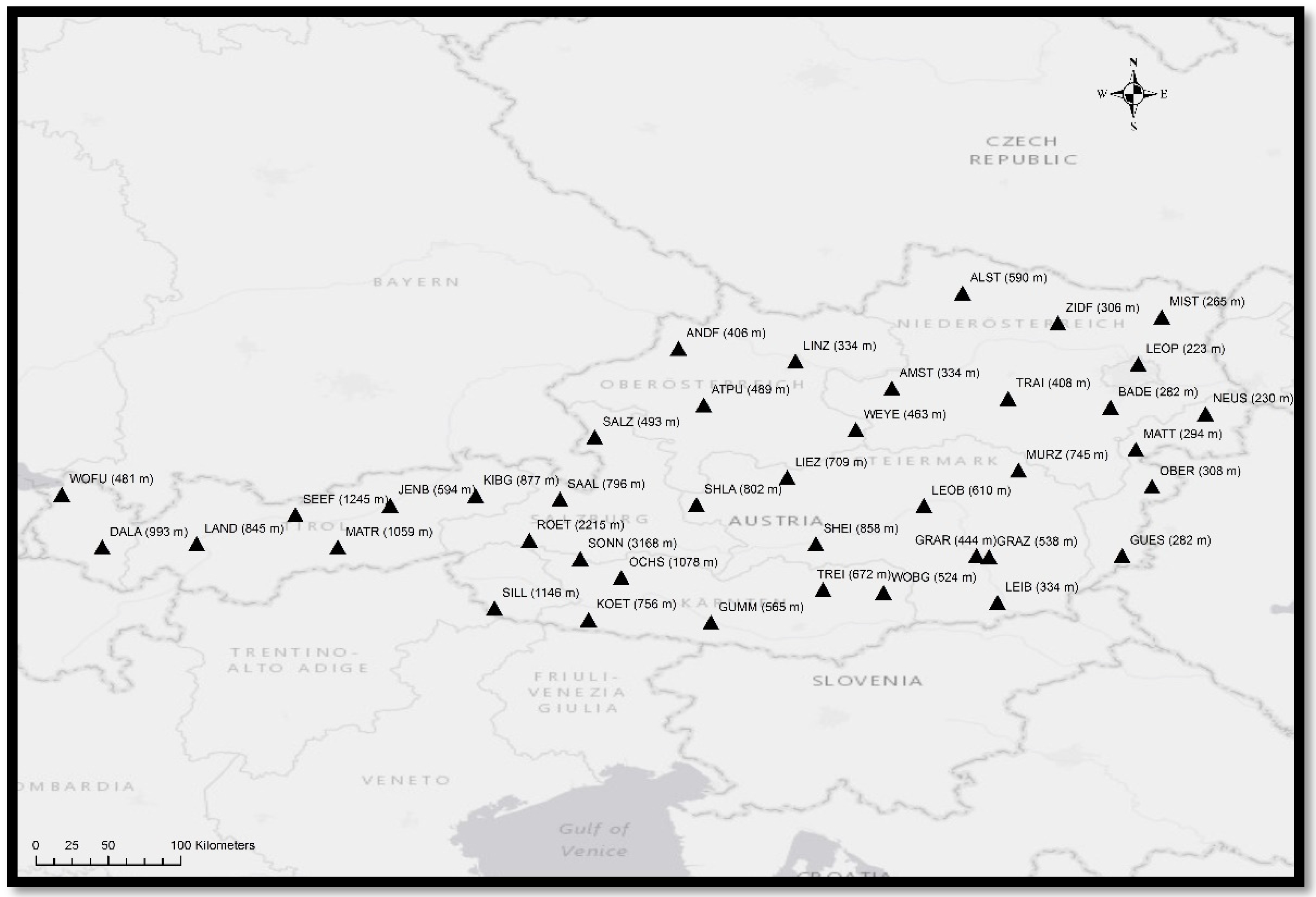
In the study, observations collected from 40 stations of the EPOSA GNSS Network were used for an assessment of the interpolation methods. The distribution of the GNSS stations is given in Figure 2.

The GNSS observations were evaluated in summer, winter, and spring seasons to observe the behavior of the interpolation methods in humid and dry periods. The meteorological parameters were obtained from the TAWES Meteorological Network for the relevant days. In order to analyze the performance of the ANN, IDW, and LIN methods, the RMSE values of the errors between the interpolated values and known values were calculated. RMSE values were obtained by the following Equation (14):

$$RMSE=\sqrt{\frac{{\displaystyle \sum _{i=1}^n{\left(ZW{D}_i^{GNSS}-ZW{D}_i^{INTERP.}\right)}^2}}{n-1}},$$

(14)

where the variable n denotes the number of observations. ZWD_i^GNSS and ZWD_i^INTERP. are the ith ZWD value estimated using GNSS data and the ANN model, respectively.

3. Results

In the first strategy, training of the artificial neural network was carried out using seven parameters, as shown in Figure 1, as input parameters for each ZWD value. ZWD values were then interpolated to each reference station with this model and a cross validation test was performed. In order to analyze the accuracy, each station was removed from the training data set and ZWD value was interpolated with the ANN model formed by the remaining stations. Afterwards, interpolated ZWD values were compared with ZWD estimated by GNSS observations. In the LIN and IDW methods, the station to be interpolated was removed from the model and the interpolation of ZWD was carried out through the surrounding stations. The same evaluations were performed for 30-station and 20-station networks in order to evaluate the effect of inter-station distance on the interpolation accuracy. The average distance between stations for a 40-station network is around 30–40 km. In the 30-station network, the distance increases to around 50–60 km. The average distance between stations of the 20-station network is around 60–70 km. In the study, correlation coefficients between ZWD values and latitude, longitude, and meteorological parameters were calculated by Equation (15) and are given in

Table 1. Correlation coefficients between meteorological parameters and zenith wet delay.

1 April	ZWD	Latitude	Longitude	H	P	T	TM	E	ZWD
	Correlation	0.29	0.54	−0.6	0.6	0.63	0.44	0.64	1
	N	959	959	959	959	959	959	959	959
2 April	ZWD	Latitude	Longitude	H	P	T	TM	E	ZWD
	Correlation	0.22	0.55	−0.88	0.89	0.88	0.62	0.88	1
	N	924	924	924	924	924	924	924	924
15 July	ZWD	Latitude	Longitude	H	P	T	TM	E	ZWD
	Correlation	0.48	0.56	−0.74	0.75	0.7	0.59	0.67	1
	N	953	953	953	953	953	953	953	953
16 July	ZWD	Latitude	Longitude	H	P	T	TM	E	ZWD
	Correlation	0.34	0.6	−0.83	0.83	0.81	0.64	0.78	1
	N	953	953	953	953	953	953	953	953
15 December	ZWD	Latitude	Longitude	H	P	T	TM	E	ZWD
	Correlation	0.49	0.4	−0.73	0.74	0.63	0.56	0.71	1
	N	956	956	956	956	956	956	956	956
16 December	ZWD	Latitude	Longitude	H	P	T	TM	E	ZWD
	Correlation	0.37	0.69	−0.53	0.56	0.3	0.73	0.58	1
	N	953	953	953	953	953	953	953	953
Mean	ZWD	Latitude	Longitude	H	P	T	TM	E	ZWD
	Correlation	0.37	0.56	−0.72	0.73	0.66	0.60	0.71	1

.

$$k=\frac{{\displaystyle \sum _{i=1}^n(x_i-\overline{x})\cdot (y_i-\overline{y})}}{\sqrt{{\displaystyle \sum _{i=1}^n{(x_i-\overline{x})}^2\cdot {\displaystyle \sum _{i=1}^n{(y_i-\overline{y})}^2}}}}$$

(15)

It can be seen that station height is negatively correlated with ZWD by 72%. The mean correlations between latitude and longitude and ZWD are 37% and 56%, respectively. The correlations between meteorological parameters and ZWD are found to be highest for P (mean 73%) and E (mean 71%) parameters. The correlation between the wet delay parameter and the height parameter and pressure parameter has almost the same absolute value and these correlation values are inverse to each other. On the other hand, the T parameter has a positive 66% correlation with ZWD. Furthermore, it can be seen that the T_M parameter has a mean correlation of 60%. According to these results, it is possible to learn that all meteorological parameters have a significant correlation with ZWD.

The T_M value is a parameter that cannot be measured directly by the meteorological stations, but it can be measured as close to reality as possible along the thickness of the troposphere with the help of meteorological balloons. In the Bevis model, the empirical equation between the surface temperature and weighted mean temperature parameters is found based on long-term radiosonde measurements. In this study, T_M values were calculated by using the Bevis model (Equation (16)) based on T₀ values obtained from TAWES stations.

T_M = 70.2 + 0.72*T₀

(16)

The water vapor pressure values (E) were calculated using the following equation by employing relative humidity values measured through in-situ observations:

$$E=\frac{RH}{100}\times E_s.$$

(17)

Here, E_s is the correction of saturated water vapor, obtained by Equation (18) and replaced in Equation (17) above.

$$E_s=\left\{\begin{array}{c}t\ge 0:0.6105\exp \left(\frac{17.269t}{237.3+t}\right)\\ t<0:0.6105\exp \left(\frac{21.875t}{265.5+t}\right)\end{array}\right\}$$

(18)

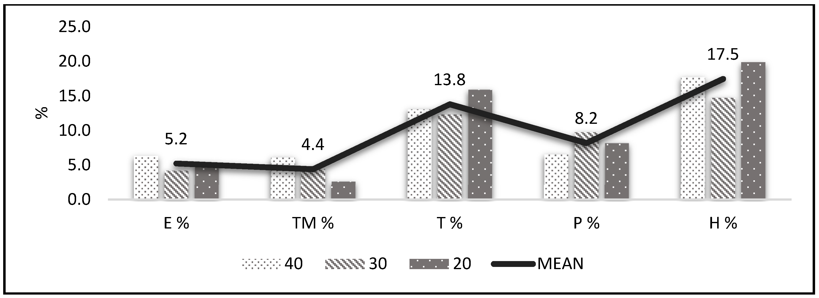
The effects of the parameters used in the ANN model on the performance of interpolation are given in Figure 3.

As shown in the Figure 3, the improvement obtained by including each parameter in the network is shown proportionally for the RMSE values. This proportional improvement can be seen separately in the graph for 40-, 30-, and 20-station networks. It is seen that the height parameter included in the ANN network provides a greater improvement than the other parameters due to it having a strong relationship with the amount of water vapor. The improvement achieved by the pressure (P) parameter is found to be less than that obtained by the elevation parameter. The contribution of the temperature (T) parameter to the success of ANN model interpolation is approximately 14%. Water vapor, which has a linear relationship with temperature, also increases the amount of wet delay in direct proportion. Therefore, the contribution of the temperature parameter included in the ANN network is higher than the weighted mean temperature and water vapor pressure. The water vapor pressure (E) contribute 5.2% to the network. The weighted mean temperature parameter (T_M) is seen to provide the least improvement, with a value of 4.4%. The calculation of T_M was carried out based on an empirical model, as previously mentioned. Therefore, it is thought that it provides less improvement compared to other parameters. Furthermore, it can be seen that these results are consistent with the correlation values between ZWD and the parameters given in Table 1. The RMSE values of the ANN (from the two-parameter model to the seven-parameter model), LIN, and IDW methods are given in Figure 4.

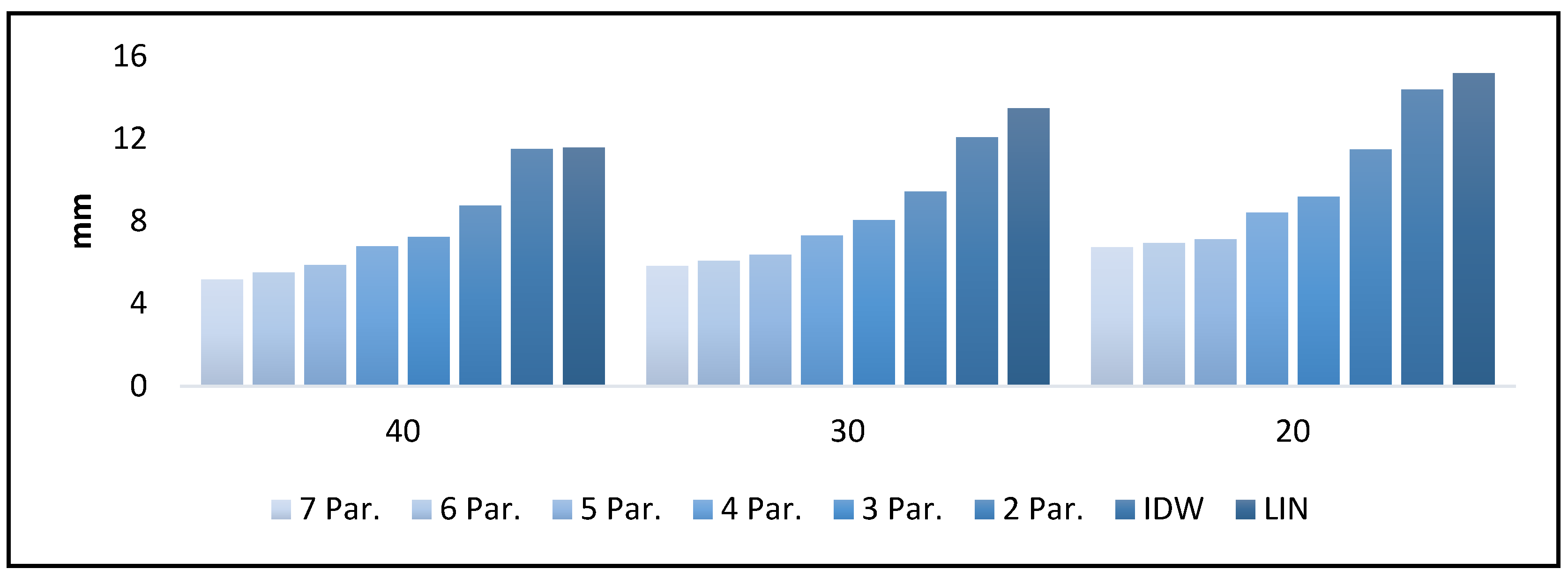
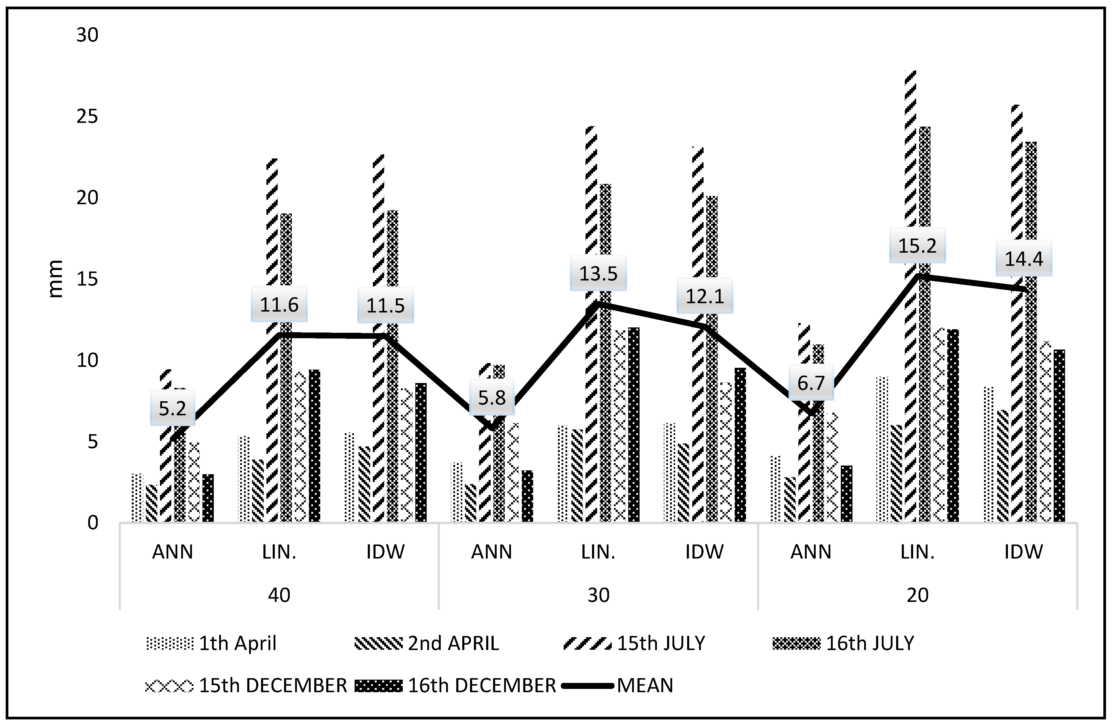
According to the RMSE values of the LIN and IDW methods, it can be seen that the conventional methods produce results close to the two-parameter ANN model. The 40-station network interpolation results with a two-parameter ANN model have an RMSE of 8.8 mm, while the LIN method has an RMSE of 11.6 mm and the IDW method has an RMSE of 11.5 mm. The results of interpolation obtained by the ANN model demonstrate that as the number of parameters increases, the RMSE values decrease. In order to evaluate the performance of all methods, the RMSE of the interpolation values was calculated for all days and is given in Figure 5.

According to Figure 5, the RMSE values of the ANN model demonstrate that an increasing distance between reference stations adversely affects the interpolation accuracy. It is found that LIN and IDW methods produce less accurate values with an increasing distance. In general, the ANN model has an RMSE of 5.2 mm for a 40-station network, 5.8 mm for a 30-station network, and 6.7 mm for a 20-station network. It is seen that LIN and IDW methods have an RMSE value of 1 cm at a 30–40 km distance in a 40-station network. It is observed that these values reached approximately 1.5 cm in 30- and 20-station networks.

4. Discussion

Interpolation of the ZWD value with a high accuracy makes significant contributions to applications in GNSS meteorology and positioning applications with the GNSS technique. For the interpolation of wet troposphere delay, analyses were carried out using the ANN, IDW, and LIN methods. Six different artificial neural network models were designed for the ANN model. In the formation of these models, the latitude, longitude, and altitude parameters, as well as meteorological parameters (temperature, pressure, water vapor pressure, and weighted mean temperature), were used. The artificial neural network model which was designed by including all parameters provided a 40% improvement compared to the two-parameter ANN model. The seven-parameter ANN model RMSE values were 5.2 mm for the 40-station network, 5.8 mm for the 30-station network and 6.7 mm for the 20-station network. The mean RMSE values of the IDW method were 11.5, 12.1, and 14.4 mm for the 40-station, 30-station, and 20-station network, respectively. The mean RMSE values of the LIN method were 11.6 mm for the 40-station network, 13.5 mm for the 30-station network, and 15.2 mm for the 20-station network. The distance between stations of the 40-station network (30–40 km) allows interpolation to be carried out at the level of a 1 cm accuracy by conventional methods. The RMSE values obtained in the 20-station network for the IDW and LIN methods increased by 16% and 11%, respectively, when compared to the 30-station network. The RMSE values obtained from the 20-station network increased by 24% for the LIN method and 20% for the IDW method compared to the 40-station network. For the ANN model, these rates were 14% and 23%. The contribution of meteorological parameters was used in the ANN model and the accuracy of ZWD interpolation was around 40%. According to these results, it could be observed that conventional methods provide an approximately 1 cm accuracy in networks with a distance between stations between 30 and 40 km and 1.5 cm for longer distances. However, in the ANN model, ZWD interpolation with an RMSE of around 6 mm can be achieved, even in networks where the distance between stations reaches 70–80 km. This contribution to the accuracy over increasing distances may help for positioning and weather forecast applications in sparse GNSS networks. In addition, the conversion factor used to calculate the PWV value from the ZWD value was approximately 0.16. Accordingly, for the ZWD with an RMSE of 6 mm, the PWV value can be obtained with an accuracy of approximately 1 mm. It has been demonstrated in previous studies that the threshold value for meteorological studies is 2–3 mm [34]. Therefore, it can be said that the accuracy of ZWD interpolation obtained by the ANN model is sufficient for meteorological estimations. According to the results, the proposed ANN model based on meteorological parameters improves the ZWD interpolation accuracy by more than 50% compared with the conventional methods. As a result, ANN algorithms can be successfully applied to meteorological estimations by choosing the optimal parameters as the input of the model. Moreover, using the ability of artificial neural networks based on different architectures may help to improve the water vapor estimation accuracy on a global scale. In future studies, regional T_M models can be used instead of the Bevis model, which has limitations due to the latitude dependency, in order to obtain a more accurate ANN structure. Furthermore, the proposed ANN model can be tested on GNSS networks located in different climatic regions of the world.

References

1. Niell, A. Global mapping functions for the atmosphere delay at radio wavelengths. J. Geophys. Res. Solid Earth 1996, 101, 3227–3246. [Google Scholar] [CrossRef]
2. Böhm, J.; Niell, A.; Tregoning, P.; Schuh, H. Global Mapping Function (GMF): A new empirical mapping function based on numerical weather model data. Geophys. Res. Lett. 2006, 33. [Google Scholar] [CrossRef] [Green Version]
3. Hopfield, H. Two-quartic tropospheric refractivity profile for correcting satellite data. J. Geophys. Res. 1969, 74, 4487–4499. [Google Scholar] [CrossRef]
4. Saastamoinen, J. Contributions to the theory of atmospheric refraction. Bull. Géodésique 1972, 105, 279–298. [Google Scholar] [CrossRef]
5. Goad, C.; Goodman, L. Modified Hopfield tropospheric refraction correction model. In Proceedings of the Fall Annual Meeting American Geophysical Union, San Francisco, CA, USA, 12–17 December 1974; p. 1106. [Google Scholar]
6. Black, H.D. An easily implemented algorithm for the tropospheric range correction. J. Geophys. Res. Solid Earth 1978, 83, 1825–1828. [Google Scholar] [CrossRef]
7. Davis, J.; Herring, T.; Shapiro, I.; Rogers, A.; Elgered, G. Geodesy by radio interferometry: Effects of atmospheric modeling errors on estimates of baseline length. Radio Sci. 1985, 20, 1593–1607. [Google Scholar] [CrossRef]
8. Askne, J.; Nordius, H. Estimation of tropospheric delay for microwaves from surface weather data. Radio Sci. 1987, 22, 379–386. [Google Scholar] [CrossRef]
9. Mendes, V. Modeling the Neutral-Atmospheric Propagation Delay in Radiometric Space Techniques; UNB Brunswick: Fredericton, NB, Canada, 1999. [Google Scholar]
10. Selbesoglu, M.O. Evaluation of Precipitable Water Vapor Derived From Global Navigation Satellite System Observations based on Troposphere Model. Feb-Fresenius Environ. Bull. 2017, 26, 3924–3929. [Google Scholar]
11. Al-Shaery, A.; Lim, S.; Rizos, C. Investigation of different interpolation models used in Network-RTK for the virtual reference station technique. J. Glob. Position. Syst. 2011, 10, 136–148. [Google Scholar] [CrossRef]
12. Gumus, K.; Selbesoglu, M.O.; Celik, C.T. Accuracy investigation of height obtained from Classical and Network RTK with ANOVA test. Measurement 2016, 90, 135–143. [Google Scholar] [CrossRef]
13. Zheng, D.; Hu, W.; Wang, J.; Zhu, M. Research on regional zenith tropospheric delay based on neural network technology. Surv. Rev. 2015, 47, 286–295. [Google Scholar] [CrossRef]
14. Ding, M. A neural network model for predicting weighted mean temperature. J. Geod. 2018, 92, 1187–1198. [Google Scholar] [CrossRef]
15. Rodrigues, E.R.; Oliveira, I.; Cunha, R.; Netto, M. DeepDownscale: A deep learning strategy for high-resolution weather forecast. In Proceedings of the 2018 IEEE 14th International Conference on e-Science (e-Science), Amsterdam, The Netherlands, 29 October–1 November 2018; pp. 415–422. [Google Scholar]
16. Benevides, P.; Catalao, J.; Nico, G. Neural Network Approach to Forecast Hourly Intense Rainfall Using GNSS Precipitable Water Vapor and Meteorological Sensors. Remote Sens. 2019, 11, 966. [Google Scholar] [CrossRef]
17. Manzato, A.; Pucillo, A.; Cicogna, A. Improving ECMWF-based 6-h maximum rain using instability indices and neural networks. Atmos. Res. 2019, 217, 184–197. [Google Scholar] [CrossRef]
18. Pereira, S.; Canhoto, P.; Salgado, R.; Costa, M.J. Development of an ANN based corrective algorithm of the operational ECMWF global horizontal irradiation forecasts. Sol. Energy 2019, 185, 387–405. [Google Scholar] [CrossRef]
19. Paras, S.M.; Kumar, A.; Chandra, M. A feature based neural network model for weather forecasting. Int. J. Comput. Intell. 2009, 4, 209–216. [Google Scholar]
20. Hayati, M.; Mohebi, Z. Application of artificial neural networks for temperature forecasting. World Acad. Sci. Eng. Technol. 2007, 28, 275–279. [Google Scholar]
21. Hung, N.Q.; Babel, M.S.; Weesakul, S.; Tripathi, N. An artificial neural network model for rainfall forecasting in Bangkok, Thailand. Hydrol. Earth Syst. Sci. 2009, 13, 1413–1425. [Google Scholar] [CrossRef] [Green Version]
22. Abhishek, K.; Singh, M.; Ghosh, S.; Anand, A. Weather forecasting model using artificial neural network. Procedia Technol. 2012, 4, 311–318. [Google Scholar] [CrossRef]
23. Gavili, S.; Sanikhani, H.; Kisi, O.; Mahmoudi, M.H. Evaluation of several soft computing methods in monthly evapotranspiration modelling. Meteorol. Appl. 2018, 25, 128–138. [Google Scholar] [CrossRef]
24. Naganna, S.R.; Deka, P.C.; Ghorbani, M.A.; Biazar, S.M.; Al-Ansari, N.; Yaseen, Z.M. Dew point temperature estimation: Application of artificial intelligence model integrated with nature-inspired optimization algorithms. Water 2019, 11, 742. [Google Scholar] [CrossRef]
25. Zheng, Y.; Feng, Y.; Bai, Z. Grid residual tropospheric corrections for improved differential GPS positioning over the Victoria GPS Network (GPSnet). Positioning 2005, 1. [Google Scholar] [CrossRef]
26. Pace, B.; Pacione, R.; Sciarretta, C.; Vespe, F. Estimating Zenith Total Delay Residual Fields by using Ground-Based GPS network. In Proceedings of the XX EUREF Symposium, Gävle, Sweden, 2–5 June 2010. [Google Scholar]
27. Webley, P.; Bingley, R.; Dodson, A.; Wadge, G.; Waugh, S.; James, I. Atmospheric water vapour correction to InSAR surface motion measurements on mountains: Results from a dense GPS network on Mount Etna. Phys. Chem. Earth Parts A/B/C 2002, 27, 363–370. [Google Scholar] [CrossRef]
28. Emardson, T.; Simons, M.; Webb, F. Neutral atmospheric delay in interferometric synthetic aperture radar applications: Statistical description and mitigation. J. Geophys. Res. Solid Earth 2003, 108. [Google Scholar] [CrossRef]
29. Janssen, V.; Ge, L.; Rizos, C. Tropospheric corrections to SAR interferometry from GPS observations. Gps Solut. 2004, 8, 140–151. [Google Scholar] [CrossRef] [Green Version]
30. Zhang, J. Precise estimation of residual tropospheric delays in a spatial GPS network. In Proceedings of the National Technical Meeting of the Satellite Division of the Institute of Navigation, ION GPS/1999, Nashville, TN, USA, 14–17 September 1999; pp. 1391–1401. [Google Scholar]
31. Schüler, T. The TropGrid2 standard tropospheric correction model. Gps Solut. 2014, 18, 123–131. [Google Scholar] [CrossRef]
32. Dach, R.; Hugentobler, U.; Fridez, P.; Meindl, M. Bernese GPS software version 5.0. Astron. Inst. Univ. Bern 2007, 640, 114. [Google Scholar]
33. Shepard, D. A two-dimensional interpolation function for irregularly-spaced data. In Proceedings of the 23rd ACM national conference, New York, NY, USA, 27–29 August 1968; pp. 517–524. [Google Scholar]
34. De Haan, S. National/Regional Operational Procedures of GPS Water Vapour Networks and Agreed International Procedures; WMO: Geneva, Switzerland, 2006; Volume 1340, p. 20. [Google Scholar]
Figure 1. Artificial neural network (ANN) models.
Applsci 09 04688 g001
Figure 2. EPOSA Global Navigation Satellite System (GNSS) Network.
Applsci 09 04688 g002
Figure 3. Contribution of meteorological parameters to ANN model accuracy.
Applsci 09 04688 g003
Figure 4. Root mean square error (RMSE) values of ANN models and linear interpolation method (LIN) and inverse distance weighted interpolation (IDW) methods.
Applsci 09 04688 g004
Figure 5. RMSE values for ANN-LIN-IDW methods.
Applsci 09 04688 g005