Helping the Visually Impaired See via Image Multi-labeling Based on SqueezeNet CNN

Abstract

This work presents a deep learning method for scene description. (1) Background: This method is part of a larger system, called BlindSys, that assists the visually impaired in an indoor environment. The method detects the presence of certain objects, regardless of their position in the scene. This problem is also known as image multi-labeling. (2) Methods: Our proposed deep learning solution is based on a light-weight pre-trained CNN called SqueezeNet. We improved the SqueezeNet architecture by resetting the last convolutional layer to free weights, replacing its activation function from a rectified linear unit (ReLU) to a LeakyReLU, and adding a BatchNormalization layer thereafter. We also replaced the activation functions at the output layer from softmax to linear functions. These adjustments make up the main contributions in this work. (3) Results: The proposed solution is tested on four image multi-labeling datasets representing different indoor environments. It has achieved results better than state-of-the-art solutions both in terms of accuracy and processing time. (4) Conclusions: The proposed deep CNN is an effective solution for predicting the presence of objects in a scene and can be successfully used as a module within BlindSys.

1. Introduction

Visual impairment is a major problem affecting many people in the world. In 2018, the World Health Organization has estimated the number of people suffering from this impairment to be 1.3 billion, of whom 36 million are blind [1]. Visually impaired (VI) individuals face many hurdles in their daily lives. They have trouble performing many of the daily actions we take for granted such as reading text, navigating the environment, or recognizing people and objects around them. In the past, VI individuals made use of white canes or guide dogs to aid them in such tasks as navigation. They rely on braille systems for reading and learning. They also rely on other people to help them from time to time especially with more complex tasks. However, technology can offer many solutions for VI individuals with a more consistent and contentious service. Early examples include refreshable braille displays, which allowed the VI to type and view text [2,3]. It is a kind of keyboard composed of cells that can be refreshed with braille characters to reflect the text on a screen. Another solution is the screen reader, which is a type of text-to-speech supplication, developed by researchers at IBM [4,5]. Other types of technological solutions include the use of robotics to aid the VI in navigation and to serve as a home assistant [6,7].

Nowadays, technology solutions based on advances in computer vision and machine learning has evolved into one of the most exciting areas of technological innovation today. The overwhelming majority of the contributions can be categorized under one of the two categories confined to navigation (i.e., by allowing more freedom in terms of mobility, orientation, and obstacle avoidance) and recognition (i.e., by providing the blind person with information related to the nature of objects encountered in his/her context). The category of research work focusing on the recognition task for blind people consists of several notable works [8,9,10,11,12,13,14]. However, many challenging issues are still unresolved due to the complex nature of indoor scenes and the need to recognize many types of objects in a short period of time for the system to be useful to a blind person. One way to reduce the complexity of the problem is not to care about providing the exact location of objects in the scene to the blind person. Instead, only detect the mere presence of the objects in the scene. Then, this problem becomes similar to what is known as image multi-labeling, or in other words assigning an image to many classes instead of just one. In this context, Mekhalfi et al. proposed a method for the detection of the presence of a set of objects based on the comparison to a set of stored images with known object contents [8]. To compare the query image to the stored images, the authors proposed to use features based on scale invariant feature transform (SIFT), the notion of a bag of words (BOW), and principal component analysis (PCA). Besides, using hand-crafted features which may not be able to describe the images well, their method relies on selecting a set of representative images to be used for comparison. However, in addition, comparing to this set of images for every query image is computationally expensive. The authors in [9] proposed another method which exploits Compressive Sensing (CS) theory for image representation and a semantic similarity metric for image likelihood estimation through learned Gaussian Process Regression (GPR) models. Malek et al. [12] used three low-level feature extraction algorithms, namely the histogram of oriented gradient (HOG), the BOW, and the local binary pattern (LBP). They merged these features using a deep learning approach, in particular an auto encoder neural network (AE), to create a new high-level feature representation. Finally, a single layer neural network was used to map the AE features into image multi-labels.

Recently there has been a major development in the field of computer vision for object detection and recognition-based deep learning approaches, in particular the set of convolutional neural networks (CNNs) [15,16,17,18]. Deep learning is a family of machine learning based on learning data representation. The learning can be supervised or unsupervised depending on the adopted architecture. The most famous deep architectures are the stacked AutoEncoder (SAE) [19], which consists in a concatenation of many AutoEncoders (AEs), a deep belief network (DBN) [20], which is based on a series of restricted Boltzmann machines (RBMs), and CNNs [21]. Deep CNNs have achieved impressive results on a variety of applications including image classification [22,23,24,25], object detection [15,16,17,18], and image segmentation [26]. Thanks to their sophisticated structure, they have the ability to learn powerful generic image representations in a hierarchical way compared to state-of-the-art shallow methods based on handcrafted features. Modern CNNs are made up of several alternating convolution and pooling layers followed by some fully connected layers. The feature maps produced by the convolution layers are usually fed to a nonlinear gating function such as the sigmoid function or the more advanced rectified linear unit (ReLU) function. The output of this activation function can then be further subjected to normalization (i.e., local response normalization) to help with generalization. The whole CNN architecture is trained end-to-end using the backpropagation algorithm [27].

Like any other classification model that learns a mapping between input data and its labels, CNNs are prone to overfitting. Overfitting refers to a model that learns the training data too well, but when it comes to the unseen testing data, it fails. Overfitting is more likely with nonparametric and nonlinear models that have more flexibility when learning a target function. CNNs are nonlinear models that have large amounts of free weights that can be learned. Thus, they have more flexibility to learn training data too well. They can learn the detail and noise in the training data to the extent that it negatively impacts the performance of the model on unseen testing data. When we have large amounts of labeled training data, then overfitting is drastically reduced. However, with small training data, overfitting is a major problem for deep machine learning. In this case, it has been shown that it is more interesting to transfer knowledge from CNNs (such as AlexNet [28], VGG-VD [29], GoogLeNet [30], and ResNet [24]) pre-trained on an auxiliary recognition task with a very large amount of labeled data instead of training a CNN from scratch [31,32,33,34]. The possible transfer learning solutions include fine-tuning the pre-trained CNN on the labeled data of the target dataset or to exploit the CNN feature representations with an external classifier. We refer the reader to [32] where the authors introduce and investigate several factors affecting the transferability of these representations.

In this work, we build a real-time deep learning solution for the image multi-labeling problem. The image multi-labeling solution is a module within a larger system, called BlindSys, that helps the visually impaired see. Through the image multi-labeling module, the visually impaired can become aware of the presence of a given set of objects in his environment. Our proposed deep learning solution is based on a light-weight pre-trained CNN called SqueezeNet that has less than 1.5 million weights. We improve the SqueezeNet architecture by resetting the last convolutional layer to free weights, replacing its activation function from a ReLU to a LeakyReLU, and adding a BatchNormalization layer thereafter. We also replace the activation functions at the output layer from softmax to linear functions. These adjustments help with the generalization capability of the network as demonstrated by the experimental results. Due to its small size, the proposed deep CNN for image multi-labeling can be trained using a fine-tuning approach with reasonable computational resources. Therefore, the main contributions of this work can be summarized as follows:

1)

A novel deep learning solution for image multi-labeling based on knowledge transfer from the pre-trained SqueezeNet CNN.

2)

The proposed CNN architecture improves the SqueezeNet CNN by using the more advanced LeakyReLU activation function and the BatchNormalization technique. It also reduces the number of weights (to less than 900,000) to combat overfitting.

3)

The proposed deep solution uses a fine-tuning approach to adapt the CNN to the new target dataset.

The rest of the paper is organized as follows. In Section 2, we give a full description of the methodology, including the problem formulation, the CNN theory, and the proposed deep CNN solution based on SqueezeNet. Section 3 presents the datasets and the experimental results. Finally, concluding remarks are given in Section 4.

2. Materials and Methods

First, this section defines the problem at hand formally. We then explain how to solve image multi-labeling using pre-trained convolutional neural networks in Section 2.2. Finally, we present our proposed solution based on the pre-trained model known as SqueezeNet.

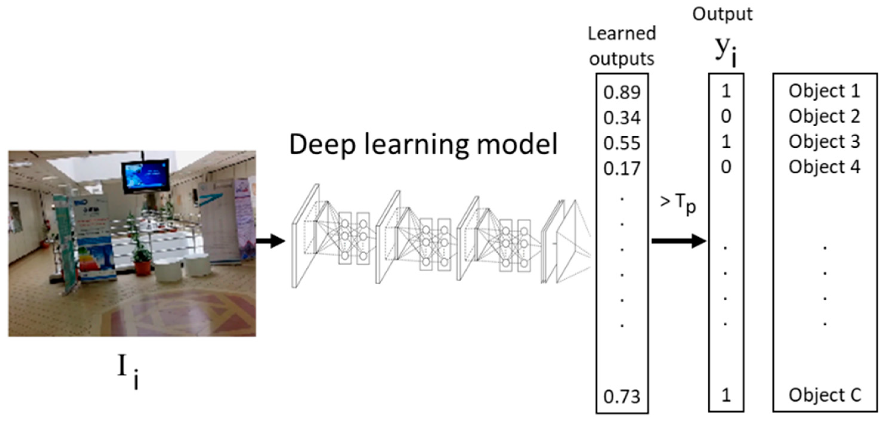
2.1. Problem Formulation

Let ${\left\{I_i,{\mathit{y}}_{\mathit{i}}\right\}}_{i=1}^n$ be a training set where $I_i\in {\mathcal{R}}^{w\times h\times 3}$ is an image of size $w\times h\times 3,$ and ${\mathit{y}}_{\mathit{i}}\in {\mathcal{R}}^{1\times c}$ is its corresponding “object indicator” vector of size $c$, which is equal to number of objects of concern. Vector ${\mathit{y}}_{\mathit{i}}$ is composed of a binary sequence where one indicated the presence of an object in the scene, while zero indicated otherwise. Let also $f_l^{\mathrm{CNN}},l=1,\dots ,L$ be a CNN model with $L$ layers pre-trained on a large amount of labeled auxiliary images from a different domain. Here, $f_l^{\mathrm{CNN}}$ refers the output of the $l^{th}$ layer. Our aim is to develop a deep learning system that can map the test images ${\left\{I_i\right\}}_{i=1}^m$ to binary vectors ${\mathit{y}}_{\mathit{i}}$ (which indicates the presence or no presence of objects) based on the available training set as well the pre-trained CNN model. Figure 1 clarifies the image multi-labeling problem further.

2.2. Deep CNN Architectures

Deep learning CNNs are composed of several layers of processing, each comprising linear as well as non-linear operators, which are learnt jointly, in an end-to-end way, to solve specific tasks [10,11]. Specifically, deep CNNs are commonly made up of four types: 1) a convolutional layer; 2) a normalization layer, 3) a pooling layer, and 4) a fully connected layer. The convolutional layer is the core building block of the CNN, and its parameters consist of a set of learnable filters. Every filter is small spatially (along width and height), but extends through the full depth of the input image. The feature maps produced via convolving these filters across the input image are fed to a non-linear gating function such as the sigmoid or ReLU functions [28].

Regarding the pooling layer, it takes small rectangular blocks from the convolutional layer and subsamples it to produce a single output from each block. There are several ways to perform pooling, such as taking the average or the maximum, or a learned linear combination of the values in the block. The main two reasons of using this layer are 1) to control overfitting and 2) to reduce the amount of parameters and computation in the network. After several convolutional and pooling layers, the high-level reasoning in the neural network is done via fully connected layers. A fully connected layer takes all neurons in the previous layer and connects it to every single neuron it has. All the weights in the CNN are learned using the well-known back-propagation technique.

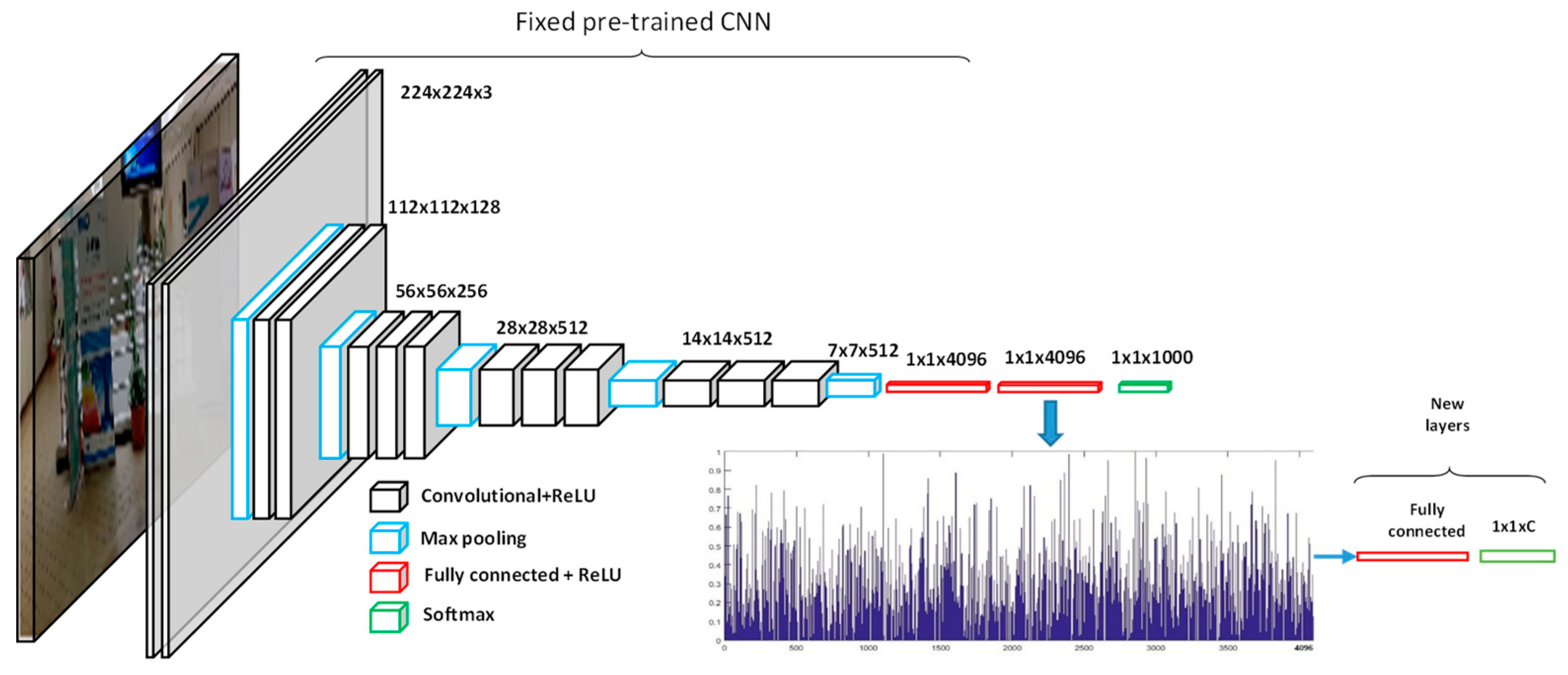
2.3. Image Multi-Labeling Based on a Pre-Trained CNN

Typically, early deep leaning solutions use a pre-trained CNN as an extractor of high level features. The complete learning model then uses extra network layers (usually fully connected layers) to adapt the network to another problem. Given the deep nature of a CNN, one can extract features at different layers. Thus, given an image $I_{\mathit{i}}$, we can generate a feature representation vector ${\mathit{x}}_i\in {\mathcal{R}}^D$ of dimension $D$ as follows:

$${\mathit{x}}_i={\mathrm{f}}_k^{\mathrm{CNN}}\left(\dots {\mathrm{f}}_2^{\mathrm{CNN}}\left({\mathrm{f}}_1^{\mathrm{CNN}}\left(I_{\mathit{i}}\right)\right)\right),\hspace{1em}i=1,\dots ,n$$

(1)

where k is a layer within the network. For example, we can use the output of the hidden fully connected (FC) layer just before the last output layer (which is used to produce a classification result in the original CNN framework), to represent the training and test images. In this case, k = L-1, where L is the total number of layers in the network. Next, the extracted feature is fed into a fully connected (dense) layer that has free trainable weights that can be trained on the new dataset at hand. Figure 2 illustrates this typical architecture.

In the extra hidden FC layer, the input ${\mathit{x}}_i\in {\Re }^D$ is mapped to the hidden representation ${\mathit{h}}_i\in {\Re }^S$ of dimension $S$ through the nonlinear activation function $f$ as follows:

$${\mathit{h}}_i=\mathrm{f}(W^{\left(h\right)}.{\mathit{x}}_i+{\mathit{b}}^{\left(h\right)})$$

(2)

where $W^{\left(h\right)}\in {\Re }^{S\times D}$ is the weight matrix, and ${\mathit{b}}^{\left(h\right)}\in {\Re }^S$ is the bias vector. Similarly, the output vector ${\mathit{y}}_i$, is computed through a nonlinear activation function F as follows:

$${\mathit{y}}_i=\mathrm{f}(W^{\left(o\right)}.{\mathit{h}}_i+{\mathit{b}}^{\left(o\right)})$$

(3)

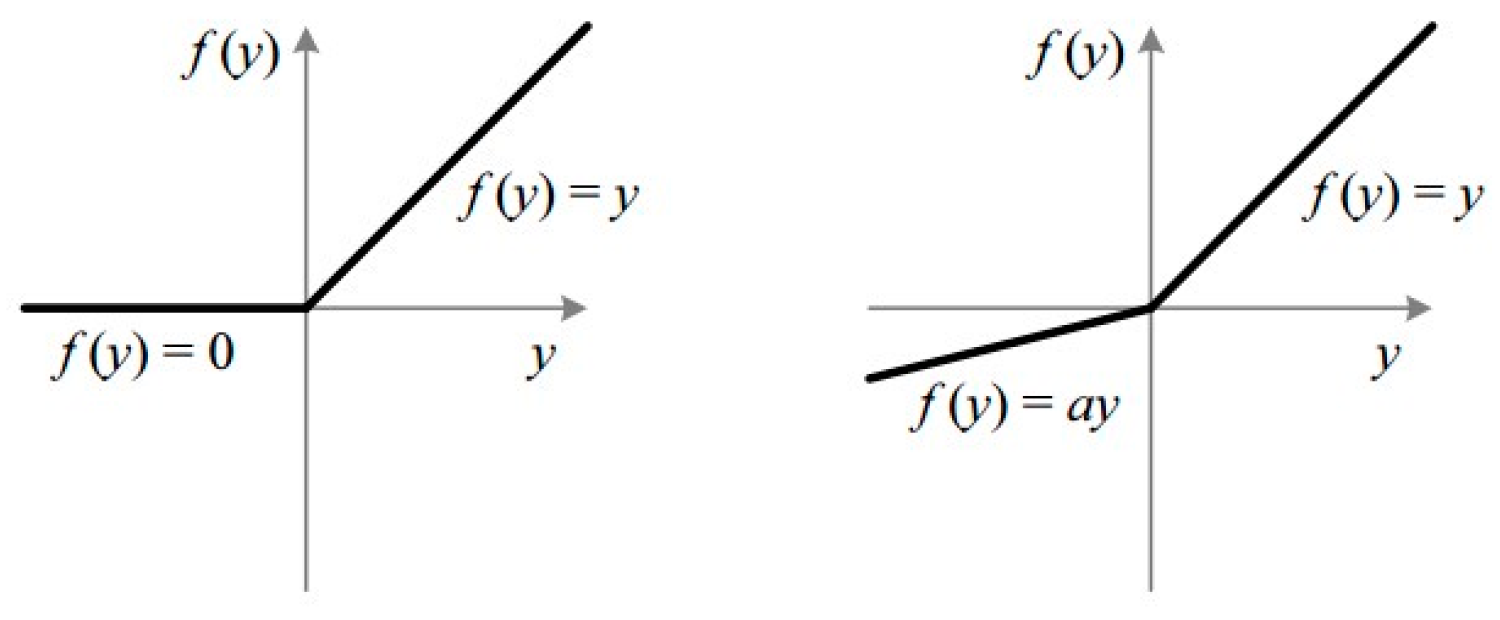
Typical choice of the activation function is the sigmoid function, i.e., $\mathrm{f}\left(v\right)=1/\left(1+\exp \left(-v\right)\right)$, or the more advanced functions called ReLU or LeakyReLU shown in Figure 3.

In order to utilize this pre-trained CNN to solve a new classification problem, we need to build the output layer so that it has as many neurons as the number of classes (typically the original CNN has an output layer with size 1000). Furthermore, for a typical classification problem, the output layer uses a softmax activation function and the categorical cross entropy loss function. Given the outputs ${\mathit{h}}_i^{\left(1\right)}$ of the last layer before the output layer, the softmax activation function produces an estimate of the posterior probability for each class label $c=1,2,\dots ,C$ as in Equation (4):

$$p\left({\widehat{y}}_i=c|{\mathit{x}}_i\right)=\frac{\exp \left({\left({\mathit{w}}_c^{\left(2\right)}\right)}^{\mathrm{T}}{\mathit{h}}_i^{\left(1\right)}\right)}{{{\displaystyle \sum }}_{j=1}^C\exp \left({\left({\mathit{w}}_j^{\left(2\right)}\right)}^{\mathrm{T}}{\mathit{h}}_i^{\left(1\right)}\right)}$$

(4)

where ${\mathit{W}}^{\left(2\right)}=\left[{\mathit{w}}_1^{\left(2\right)} {\mathit{w}}_2^{\left(2\right)}\dots {\mathit{w}}_C^{\left(2\right)}\right]\in {\Re }^{d^{}\times C}$ are the weights of the softmax layer and the superscript ${(·)}^{\mathrm{T}}$ refers to the transpose operation. This softmax activation function turns the outputs of the neurons in the last layer into probabilities by ensuring that their total sum is equal to one. This is important for classification problems because we expect only one neuron to output one (because each input image must be assigned to one class) while the rest will be zero. However, it is not appropriate for image multi-labeling because we expect many neurons to output the value one and hence the sum will not be equal to one. Thus, we use other activation functions, such as linear or sigmoid, in the output layer and optimize the mean squared error (MSE) loss function, similar to deep models for regression problems. The linear activation is more appropriate because it has a derivative equal to one, which is preferable for the backpropagation algorithm used during training. Furthermore, the linear function is not limited to the interval $\left[0,1\right]$ like the sigmoid function, so each output neuron is free to estimate values below or above the correct outputs of zero or one.

To train the neural network, we use the back propagation technique and minimize the following cost function [35]:

$${\mathcal{L}}_2\left({\mathsf{\theta }}_{NN}\right)=\frac{1}{2n}{{\displaystyle \sum }}_{i=1}^n{{\displaystyle \sum }}_{k=1}^C\Vert {\mathit{y}}_i-{\mathsf{\theta }}_{NN}{\left(x_i\right)}_{}{\Vert }^2+\frac{\lambda }{2}\left({{\displaystyle \sum }}_{l=1}^H\Vert W^{\left(h\right)}{\Vert }_F^2+{{\displaystyle \sum }}_{o=1}^c\Vert W^{\left(o\right)}{\Vert }_F^2\right)$$

(5)

where ${\mathsf{\theta }}_{NN}\left(x_i\right)$ is the output of the NN for an input $x_{\mathit{i}}$, $W^{\left(h\right)}$ and $W^{\left(o\right)}$ are the weights of the hidden layer and the output layer, respectively, and $H$ is the size of the hidden layer. The first term of (1) refers to the mean squared error between the estimated labels and the training labels, while the second term is the weight decay penalty that helps to prevent overfitting. Note also that $n$ is the number of training samples, and $C$ is the output vector size (the number of objects to be recognized). The estimation of the vector of parameters ${\mathsf{\theta }}_{NN}=\{W^{\left(h\right)},W^{\left(o\right)}\}$ of the NN starts by initializing the weights to small random values. The cost (1) is then minimized with a min-batch gradient descent algorithm [36].

At test time, we feed each test image to the CNN and assume that an output node $j$ having a predicted value larger than a given threshold (for example, 0.5) indicates the presence of the object $j$. We call this parameter the presence threshold $T_p$.

2.4. The Proposed Solution Based on the SqueezeNet CNN

During training on the new given dataset, the weights of the pre-trained CNN are either fixed or allowed to be updated. The latter case is known as fine-tuning and is obviously more time-consuming due to the large number of weights that need to be optimized. For example, successful CNNs such as AlexNet CNN [28] and the VGG-very-deep-16 CNN model [29] have more than 60 and 138 million weights, respectively. This makes them quite difficult to fine-tune for typical low-end workstations. Furthermore, because this image multi-labeling module is running on a mobile device, computational resources are limited, and hence execution time of the solution at test time must be as fast as possible. That is why, we have selected a much lighter pre-trained CNN, called SqueezeNet, that has less than 1.5 million weights, yet its accuracy is close to that of the AlexNet CNN [28].

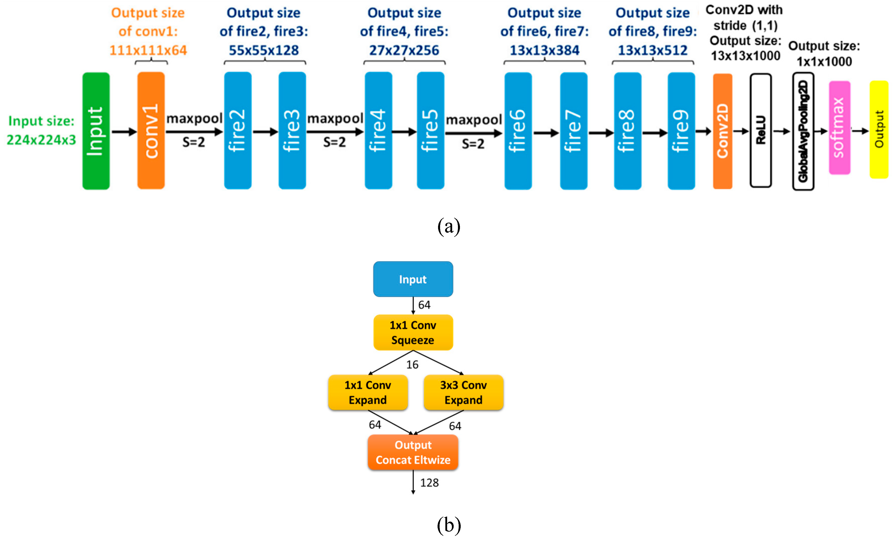
Figure 4a shows the architecture of SqueezeNet. It has 26 convolutional layers (with 34 other types of layers) and about 860 million multiply-accumulate operations compared to 1140 million for AlexNet [28]. With the help of model compression techniques, SqueezeNet has a file size of less than 0.5 MB (510 times smaller than AlexNet). SqueezeNet also accepts images of variable size (as low as 48 × 48) without the need for resizing, albeit 224 × 224 is still the ideal size. All these properties make it suitable for us to build and train our solution.

The building block of SqueezeNet is called the fire module, illustrated in Figure 4b. It contains two layers: a squeeze layer and an expand layer. A SqueezeNet stacks a bunch of these fire modules and a few pooling layers. The squeeze layer decreases the size of the feature map, while the expand layer increases it again. As a result, the same feature map size is maintained. Another pattern is increasing depth, while reducing the feature map size to obtain a high level abstract. This is accomplished through increasing the number of filters and using a stride of two in the convolutional layers.

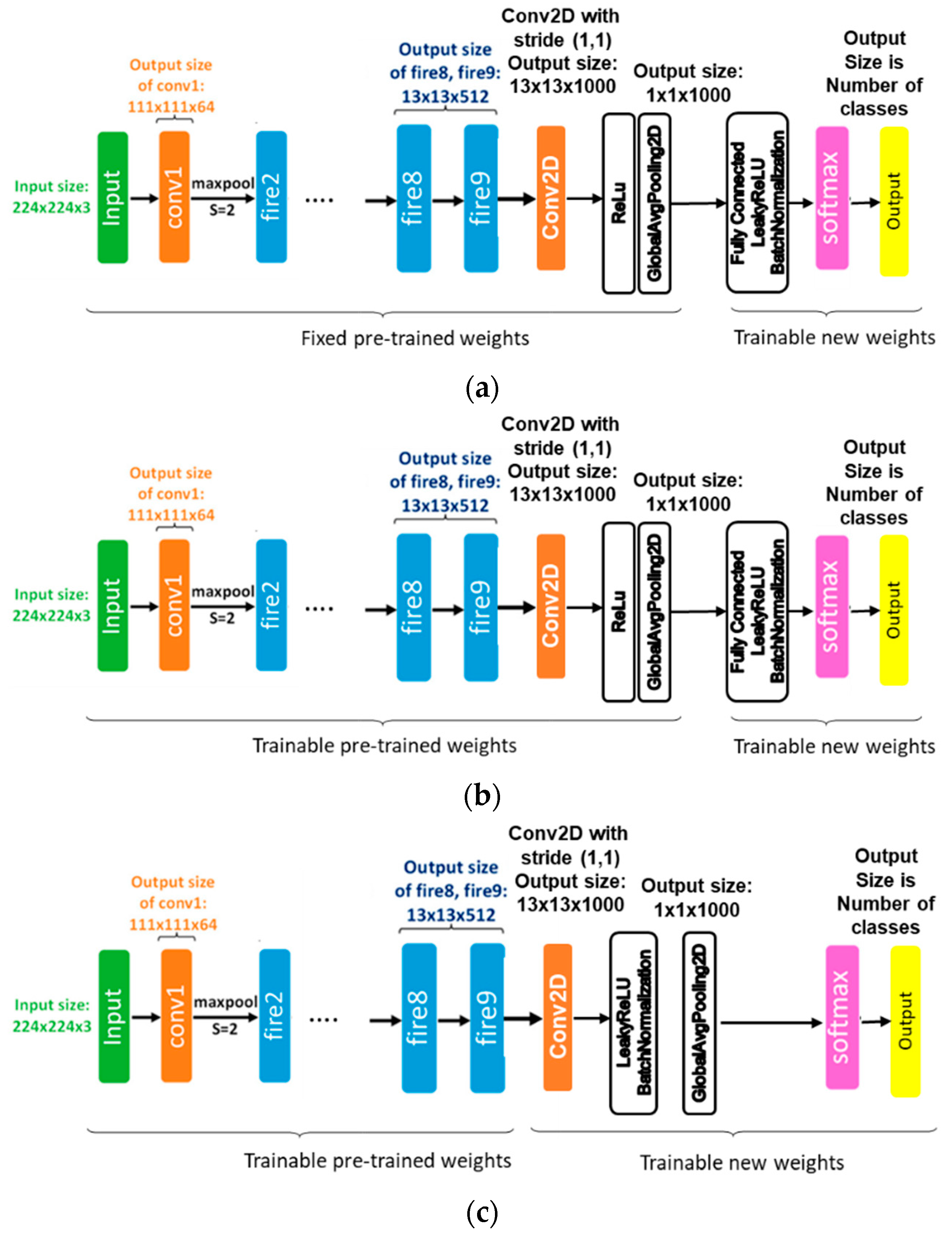
In this work, we propose a solution for the image multi-labeling problem based on fine-tuning an improved version of a pre-trained SqueezeNet CNN. In particular, we designed two improved SqueezeNet models to be used with the fine-tuning approach. We also build a base model or Model 1, illustrated in Figure 5a, that uses the pre-trained SqueezeNet as a feature extractor (i.e. its weights are fixed) and adds a fully connected layer for adapting to the given dataset. The other two improved models, referred to as Model 2 and Model 3, are illustrated in Figure 5b,c, respectively. In Model 2, we fine-tune Model 1, by making all weights of the SqueezeNet layers trainable. In Model 3, we get rid of the extra FC layer of Model 1 and reset the last convolutional layer of the SqueezeNet model to random weights. Removing the FC layer has the advantage of reducing the weights of the deep network, which consequently decreases computational costs. Resetting the weights of the last convolutional layer improves the generalization capability and affords a greater chance for the network to adapt to the new dataset. Furthermore, in all models above, we replaced the ReLU activation function of the hidden layer with new weights with the more advanced LeakyReLU activation function. We then inserted a BatchNormalization layer thereafter to fight overfitting and improve generalization capability of the network. This was not present in the original SqueezeNet model.

The BatchNormalization layer was introduced back in 2014 in the second version of GoogLeNet by Szegedy et al. [37]. BatchNormalization is similar to the concept of standardization (make the data have zero mean and sometimes also unit standard deviation) of the network input, which is a common thing to do before using a CNN on any data. BatchNormalization does the same thing inside the CNN. Specifically, we add a normalization layer after the convolutional layer, which makes the data in the current training batch (data is divided in batches to make sure it fits in computer RAM) follow a normal distribution. This way the model focuses on learning the patterns in the data and is not misled by large values in it. This in turn helps with combating overfitting and increasing the generalization ability of the network. Another advantage of the BatchNormalization technique is that it allows the model to converge faster in training and hence allows us to use higher learning rates.

The proposed solution fights overfitting by transferring the knowledge from a CNN pre-trained on a large auxiliary dataset (namely ImageNet), instead of training it with random initial weights. In addition, we also combat overfitting by reducing the number of free weights and hence reducing the flexibility of the network so that it does not learn the small details or noise in the dataset. Finally, the new BatchNormalization technique introduced inside the network improves the generalization ability of the network and fights overfitting, because it forces all feature values inside the network to be within the same small range (zero to one), instead of having the flexibility to use feature values as large as it wants in order to fit the training data.

3. Experimental Results

This section presents the experimental work of this paper. As we mentioned before, this work is part of a larger project, called BlindSys, that aims at designing an IT system to help the visually impaired perform important tasks in their lives. This system is also the source of one of the datasets used in this paper. As a result, we first present this IT system in the next subsection. After that, we describe the image datasets used in the paper and some experimental setup issues. Finally, we present the results and compare them to state-of-the-art methods.

3.1. BlindSys: A Smart IT Solution to Assist the Visually Impaired

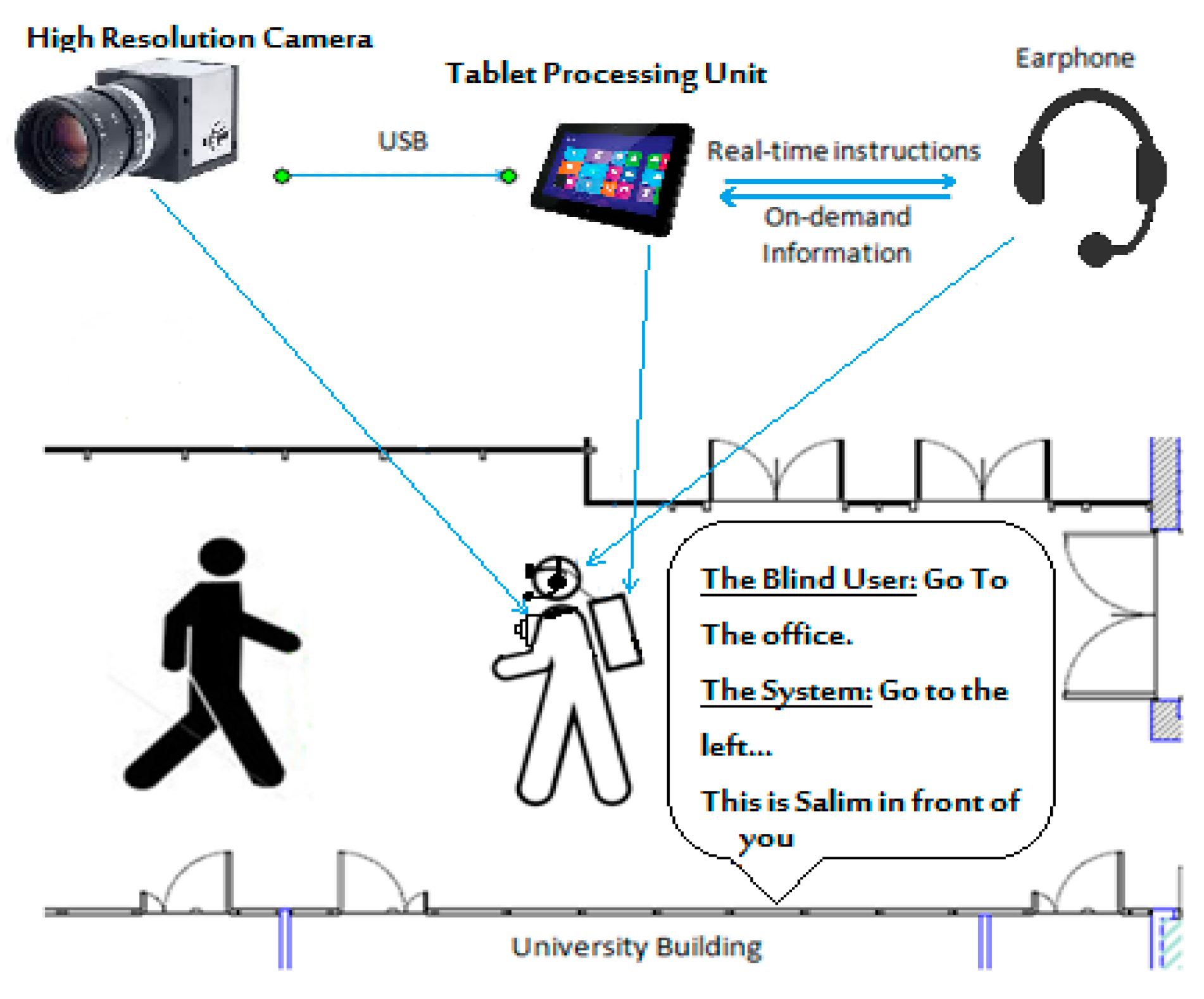
Figure 6 shows an overview of the BlindSys system for guiding VI people and helping them recognize objects and text in indoor environments. The BlindSys hardware is composed of a high resolution camera that is mounted at the chest of the VI person, a wireless headphone for voice communication with the VI user, and a mobile device that houses the BlindSys software and enables interface with the system.

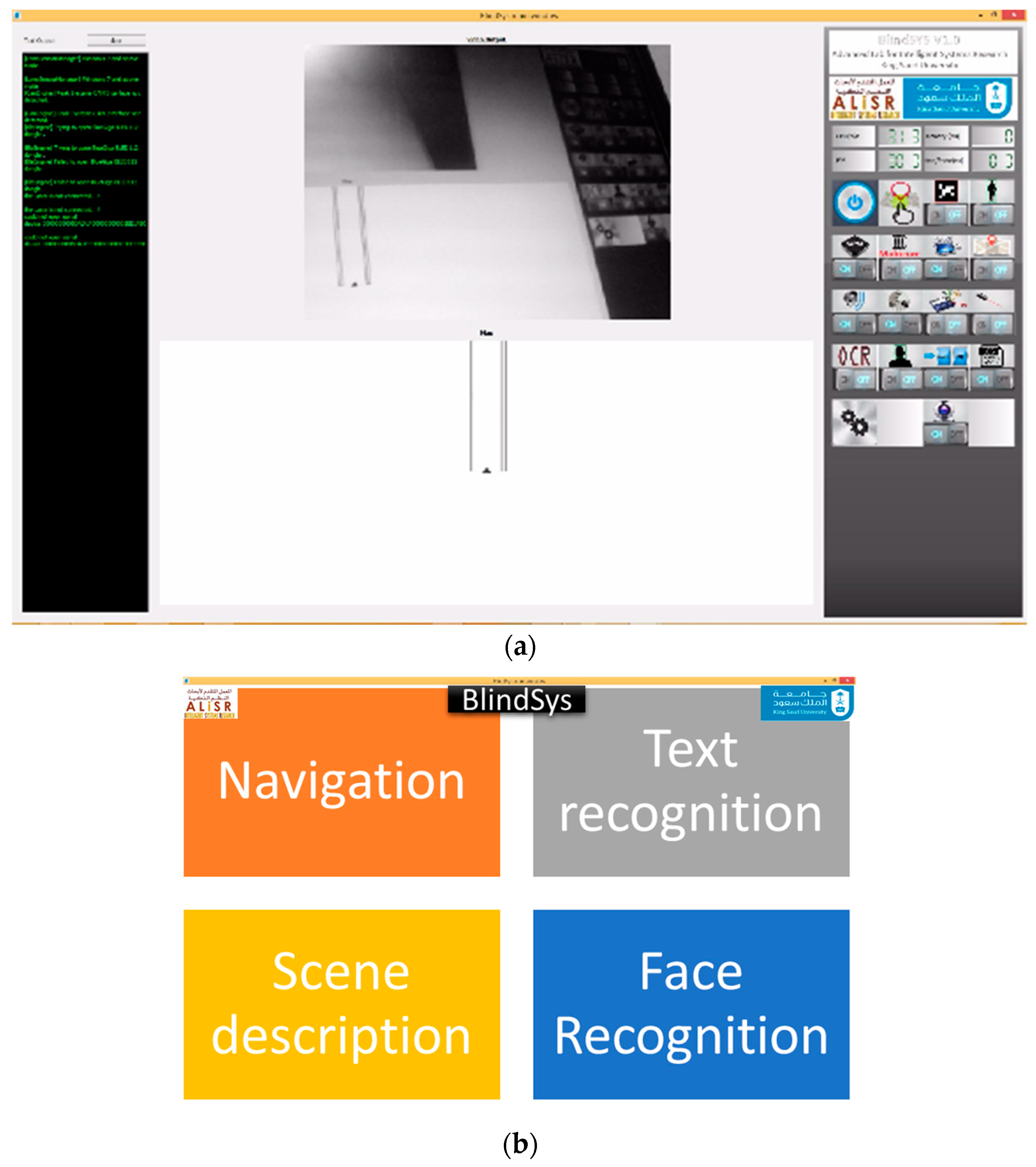
The VI user can use the system via voice commands or through a graphic user interface (GUI) to select one of four functions: 1) indoor navigation, 2) text detection and recognition, 3) scene description, or 4) face detection and recognition. Indoor navigation operates on the video stream in real time, while the other functions operate on a single image captured upon request from the video stream. To ease operation of the system, the mobile device has the simple GUI shown in Figure 7b, where the whole screen is divided into four large buttons. The VI user can press the buttons simply by touching an area close to the corners of the device. In order to avoid accidental touching, the VI user should tap the button twice consecutively. BlindSys has another main GUI, shown in Figure 7a, that can be used for testing and operator support. All processing results are communicated to the VI user via voice using text-to-speech synthesis.

The BlindSys software is based on three main parts. 1) The main application contains the application GUI and the business logic under it that manipulates all the gathered information to give navigation details to the user (video extracted information, IMU (inertial measurement unit) information, and so on). 2) Auxiliary applications that are independent from the main application are responsible for performing other functions such as OCR, face recognition, scene description, and so on. 3) Libraries are used to implement the different parts of the main application or the auxiliary applications. They are linked to the application statically or dynamically.

The scene description module can detect the presence of a set of objects in a scene image without giving exact locations. The module can detect a set of 15 objects that are commonly found in an indoor environment.

3.2. Dataset Description

The experiments in this paper use four datasets of multi-labeled images for evaluating the efficiency of the proposed deep learning solution. The first two datasets pertain to the college of the computer and the information sciences building at the King Saud University (KSU), Saudi Arabia. They have been collected by our team using the BlindSys system described in Section 3.1. The second two datasets were collected by the authors of [8] in two different buildings of the University of Trento, Italy. The cameras used to capture these images are from a company called IDS-imaging [38]. For the KSU datasets, the camera used was a UI-1220SE -C-HQ, USB 2.0, CMOS, 87.2 fps, 752 × 480, 0.36 MPix, 1/3″, ON Semiconductor, Global Shutter. For the UTrento datasets, the camera used was a UI-1240LE -C-HQ, USB 2.0, CMOS, 25.8 fps, 1280 × 1024, 1.31 MPix, 1/1.8″, e2v, Global Shutter, Global Start Shutter, Rolling Shutter. Both cameras were equipped with a KOWA LM4NCL 1/2″, 3.5 mm, F1.4 manual IRIS C-Mount lens from RMA Electronics Inc. [39]. The details of these four datasets are given in

Table 1. Details of the four datasets of multi-labeled images used in the work.

Dataset	Train/Test Sizes	Objects Considered
KSU1	161/159	pillar, fire extinguisher/hose, trash can, chairs, external door, hallway, self-service, reception, didactic service machine, display screen, board, stairs, elevator, laboratory, internal door
KSU2	86/88	board, fire extinguisher/hose, trash cans, chairs, external door, didactic service machine, self-service, reception, cafeteria, display screen, pillar, stairs, elevator, prayer room, internal door
UTrento1	58/72	external window, board, table, external door, stair door, access control reader, office, pillar, display screen, people, ATM, chairs, bins, internal door, and elevator
UTrento2	61/70	stairs, heater, corridor, board, laboratories, bins, office, people, pillar, elevator, reception, chairs, self-service, external door, and display screen

, which also presents the list of objects considered in every dataset.

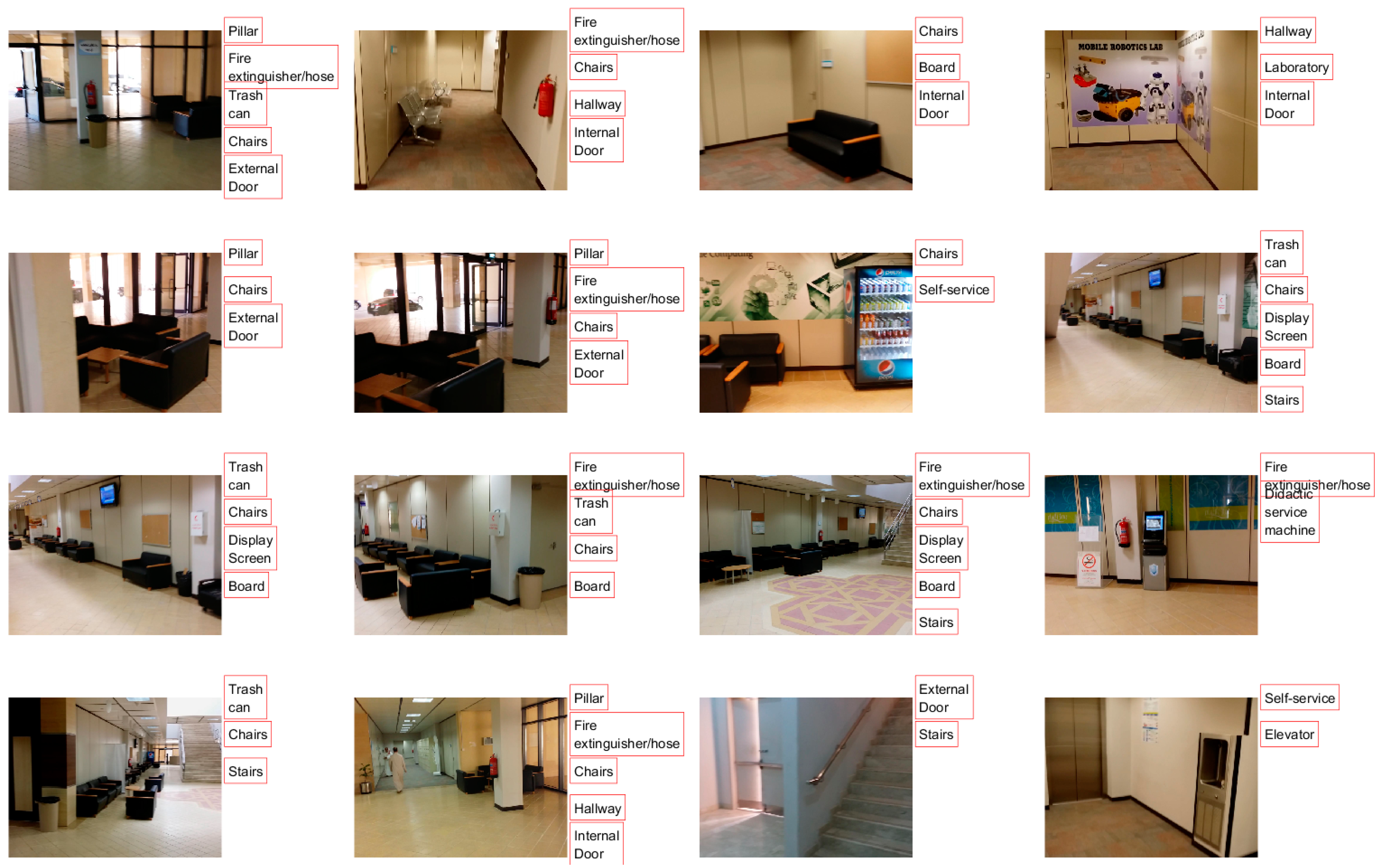
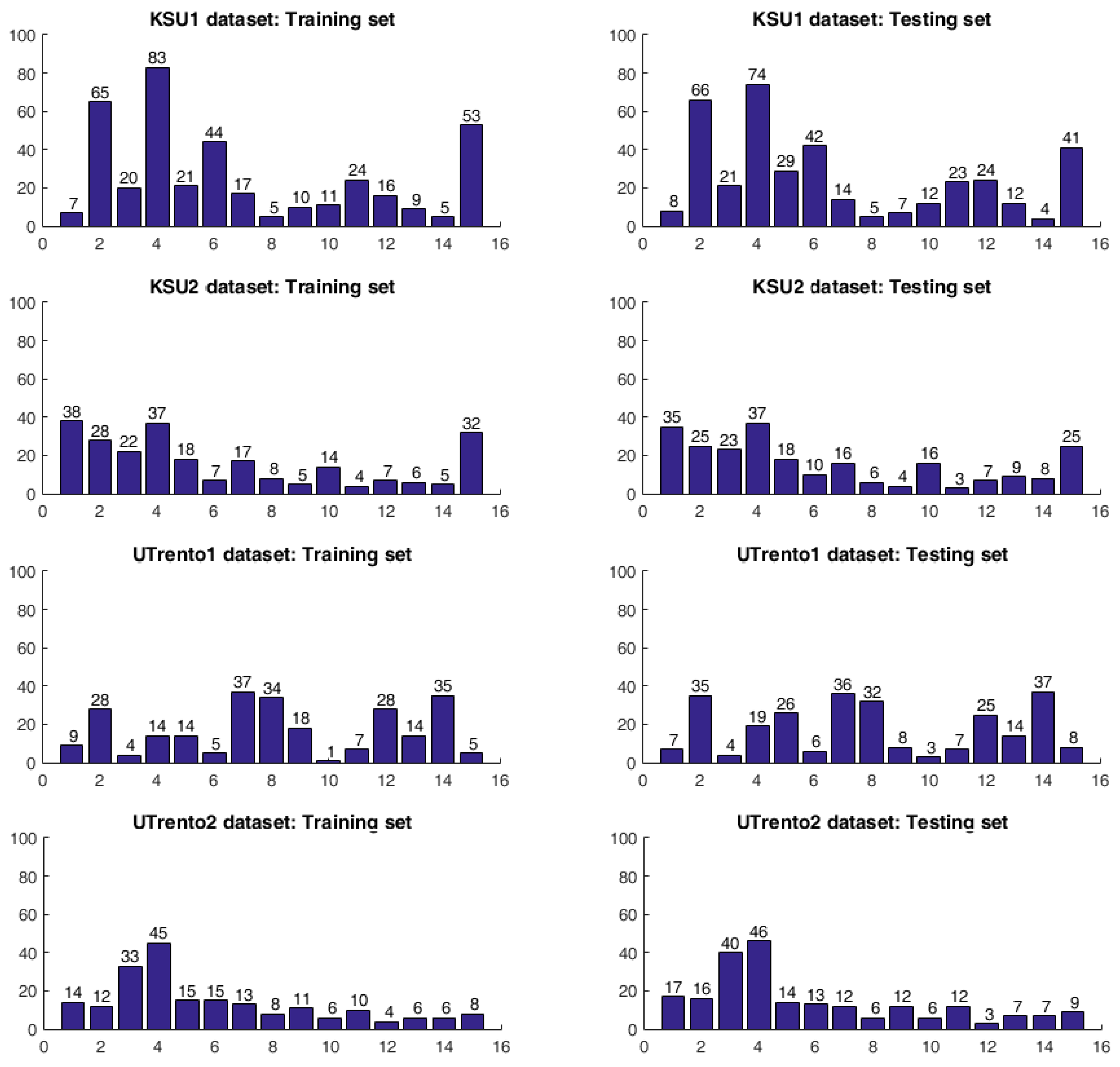
The King Saud University 1 (KSU1) dataset is composed of 320 images, divided into 161 training images and 159 testing images. The King Saud University 2 (KSU2) dataset is composed of 174 images, divided into 86 training images and 88 testing images. The University of Trento 1 (UTrento1) dataset accounts for a total of 130 images acquired in two separate daytimes (morning and evening), and these were split into 58 training images (i.e., for training the NN model) and 72 for testing purposes. Finally, the University of Trento 2 (UTrento2) dataset is composed of 131 images, divided into 61 training images and 70 testing images. It is noteworthy that the training images for all datasets were selected in such a way to cover all the predefined objects in the considered indoor environment. Thereupon, we have selected the objects deemed to be the most important ones in the considered indoor environments. 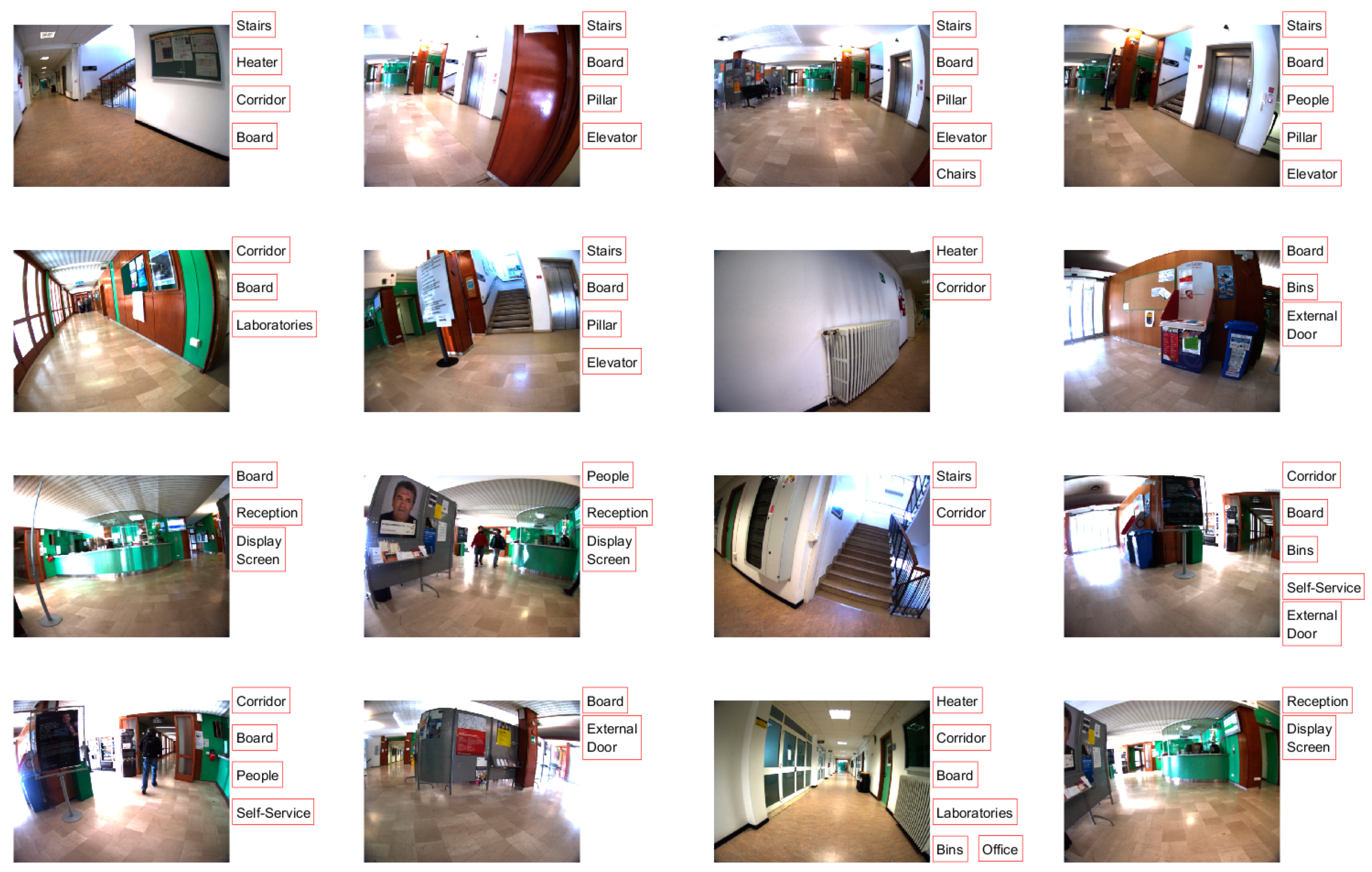Figure 8 and Figure 9 show sample images from the KSU2 and UTrento2 datasets with the list of objects contained within. Furthermore, Figure 10 presents the number of occurrences of objects in the training set and the test set of every dataset.

3.3. Experimental Setup

We implemented the proposed deep CNN solution for image multi-labeling in the Keras environment, which is a high level neural network application programming interface written in Python. We set the number of epochs to 100 and fixed the mini-batch size to 16. Additionally, we set the learning rate of the Adam optimization method to 0.0001. Regarding the exponential decay rates for the moment estimates and epsilon, we use the following default values: 0.9, 0.999, and 1e-8 respectively.

The datasets contain images of size 640 × 480. Rescaling the images to the usual size of 224 × 224 is not necessary because the SqueezeNet model is able to accept images of different sizes directly. In fact, this is one the advantages of the SqueezeNet model. Based on the input size of 640 × 480, Model 3, presented in Figure 5c, now has a low number of weights between 756,559 to 858,191 only.

The efficiency of the proposed framework is expressed in terms of the measures known as sensitivity (SEN), specificity (SPE), and their average (AVG) defined in [9,40]. SEN expresses the probability of correct detection of the presence of an object, while SPE expresses the probability of correct detection of the absence of an object, respectively. They are computed as follows:

$$\mathrm{SEN}=\frac{True Positives }{True Positives + False Negatives}$$

(6)

$$\mathrm{SPE}=\frac{True \mathrm{Negatives}}{True \mathrm{Negatives}+ False \mathrm{Positives}}$$

(7)

$$\mathrm{AVG}=\frac{SEN+ SPE}{2 }$$

(8)

All experiments are conducted on an HP-laptop with an Intel Core i7-7700HQ CPU of 2.80 GHz, 16 GB of RAM, and the NVIDIA graphics card GeForce GTX 1050 Ti with a 4 GB dedicated memory.

3.4. Results of the Proposed Deep Solution for Image Multi-Labeling

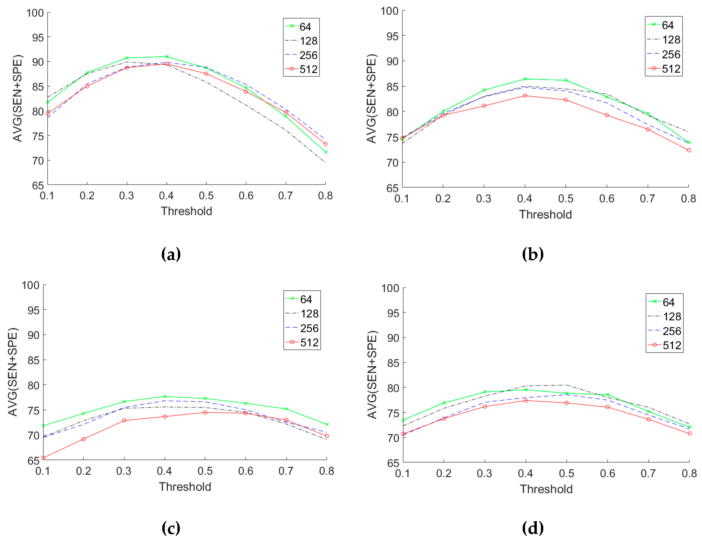
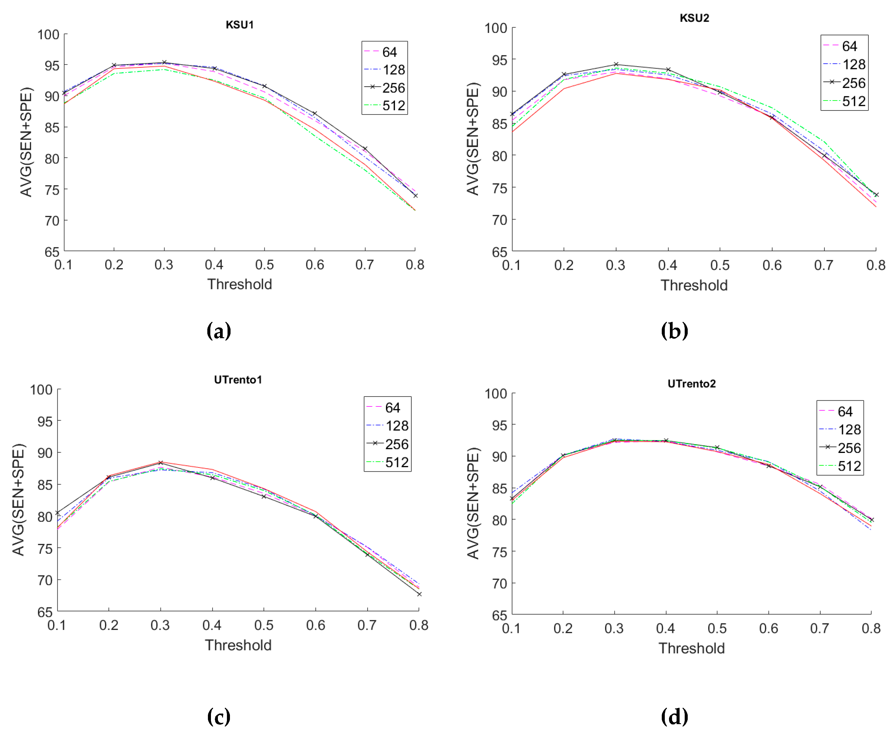
First, we present the results for the baseline model (Model 1) shown in Figure 5a based on the SqueezeNet CNN with fixed pre-trained weights. We perform sensitivity analysis for this model by varying the presence threshold $T_p$ in a range from 0.1 to 0.8 with a step size of 0.1 and by varying the hidden layer size as the following values 64, 128, 256, or 512. Figure 11 shows the analysis for the different datasets. The first observation in these figures is that a presence threshold value equal to 0.5 does not provide the most accurate results. In fact, a $T_p=0.4$ gives us the highest AVG score result overall. Secondly, in terms of the optimal hidden layer size, we can see from the figures that a hidden layer size between 64 and 128 is the most appropriate when considering all datasets.

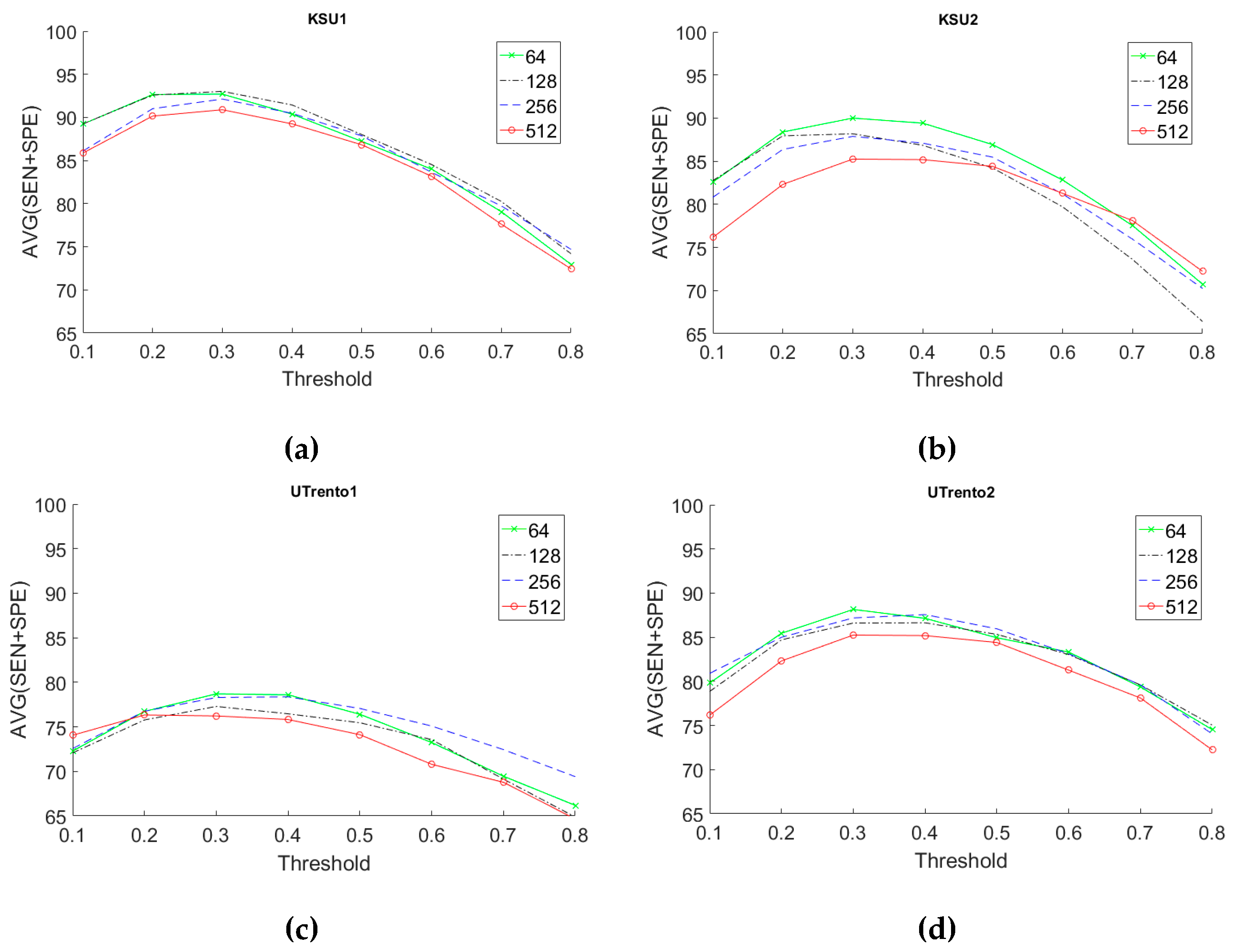
Next, we present the results of fine-tuning Models 2 and 3 shown in Figure 5b,c, respectively. Figure 12 and Figure 13 gives sensitivity analysis for Models 2 and 3, respectively. As can be seen, Model 3 gives us the best performance in terms of AVG score. Moreover, in general, a presence threshold $T_p=0.3$ is the best choice considering all datasets. The number of filters for the CONV2D layer in Model 3 does not significantly affect the results. Therefore, we selected a number equal to 256 that gives good results for most datasets, but keeps processing time per test image low.

3.5. Comparison to the State of the Art

Table 2. Comparison to state-of-the-art methods.

Dataset	Method	SEN	SPE	AVG	Time(s)
KSU 1	EDCS + GPR [9]	73.82	80.53	77.18	>1
	MR random projection [13]	71.65	94.81	83.23	0.035
	Pre-trained GoogLeNet [13]	73.56	97.95	85.75	0.064
	Fine-tune improved SqueezeNet [ours]	94.14	96.54	95.34	0.024
KSU 2	EDCS + GPR [9]	64.46	72.91	68.69	> 1
	MR random projection [13]	70.00	92.33	81.16	0.037
	Pre-trained GoogLeNet [13]	67.76	95.91	81.84	0.067
	Fine-tune improved SqueezeNet [ours]	94.51	93.79	94.15	0.029
UTrento1	SURF + GPR [9]	71.16	100.00	85.58	1.17
	EDCS + GPR [9]	69.66	80.19	74.93	1.08
	MR random projection [13]	71.16	83.20	77.18	0.037
	Pre-trained GoogLeNet [13]	61.79	96.55	79.17	0.068
	AE fusion of HOG + BOW + LBP [12]	89.51	81.3	85.41	0.022
	Fine-tune improved SqueezeNet [ours]	88.14	88.49	88.31	0.013
UTrento2	SURF + GPR [9]	77.72	100.00	88.86	1.17
	EDCS + GPR [9]	70.00	90.12	80.06	1.2
	MR random projection [13]	77.18	91.41	84.30	0.037
	Pre-trained GoogLeNet [13]	67.27	98.55	82.91	0.066
	AE fusion of HOG + BOW + LBP [12]	90.00	90.12	90.06	0.022
	Fine-tune improved SqueezeNet [ours]	94.91	89.97	92.44	0.014

presents a comparison between the proposed method and the state-of-the-art methods based on compressive sensing and Gaussian process regression (CS + GP) [9], SURF feature matching, and Gaussian process regression (SURF + GPR) [9], multi-resolution random projection (MR-random-proj) [13], fine-tuning of GoogLeNet [13], and AE fusion of HOG + BOW + LBP features [12]. These results are obtained using the proposed Model 3 with a hidden layer size of 256, and a presence threshold of 0.3, as suggested by the sensitivity analysis.

The results in Table 2 clearly show the superiority of the proposed method for all datasets, not only in terms of AVG accuracy but also in terms of execution time per image. This is mainly due to the effectiveness of the image features extracted with the help of the pre-trained SqueezeNet CNN and the improvements that we have proposed for the architecture.

4. Discussion

The results achieved in this study indicate clearly the power of SqueezeNet CNNs in extracting highly descriptive features from images, despite its small size. The improvements that we have proposed for the architecture enhanced the results significantly compared to the typical techniques for utilizing a pre-trained CNN. For example, a pre-trained GoogLeNet has been proposed in [13], but the method of fine-tuning it did not produce good results [13]. The reasons for this are several: 1) GoogLeNet has more weights (more than seven million), which requires larger datasets for training, and 2) GoogLeNet requires that the images be of size 224 × 224, which means all images have to be resized from the original size of 640 × 480 to 224 × 244. This modifies the aspect ratio of the images and causes deterioration in the classification accuracy of the network. When it comes to the SquezeNet architecture used in this study, no resizing of images is needed.

Table 3. Detailed results per object using Model 3 with the CONV2D layer size = 256 and $T_p=0.3$.

KSU1			KSU2
Objects	# Occ	AVG	Objects	# Occ	AVG
pillar	7	93.75	board	38	79.10
fire extinguisher/hose	65	92.44	fire extinguisher/hose	28	92.70
trash can	20	94.41	trash cans	22	91.73
chairs	83	90.12	chairs	37	85.22
external door	21	92.89	external door	18	95.29
hallway	44	93.86	didactic service machine	7	97.97
self-service	17	94.37	self-service	17	90.45
reception	5	99.77	reception	8	98.11
didactic service machine	10	92.2	cafeteria	5	97.74
display screen	11	99.08	display screen	14	98.61
board	24	92.92	pillar	4	99.12
stairs	16	96.7	stairs	7	97.90
elevator	9	99.59	elevator	6	98.29
laboratory	5	100.00	prayer room	5	81.06
internal door	53	84.59	internal door	32	78.38
-	SEN	94.14	-	SEN	94.51
-	SPE	96.54	-	SPE	93.79
-	AVG	95.34	-	AVG	94.15
UTrento1			UTrento2
Objects	# Occ	AVG	Objects	# Occ	AVG
external window	9	81.49	stairs	14	98.26
board	28	85.90	heater	12	94.79
table	4	98.09	corridor	33	95.54
external door	14	91.03	board	45	79.96
stair door	14	90.70	laboratories	15	86.70
access control reader	5	79.17	bins	15	84.32
office	37	88.33	office	13	95.80
pillar	34	92.19	people	8	66.09
display screen	18	90.31	pillar	11	98.56
people	1	50.00	elevator	6	99.17
ATM	7	94.33	reception	10	95.63
chairs	28	84.97	chairs	4	99.18
bins	14	84.25	self-service	6	87.86
internal door	35	76.57	external door	6	95.71
elevator	5	91.25	display screen	8	95.37
-	SEN	88.14	-	SEN	94.91
-	SPE	88.49	-	SPE	89.97
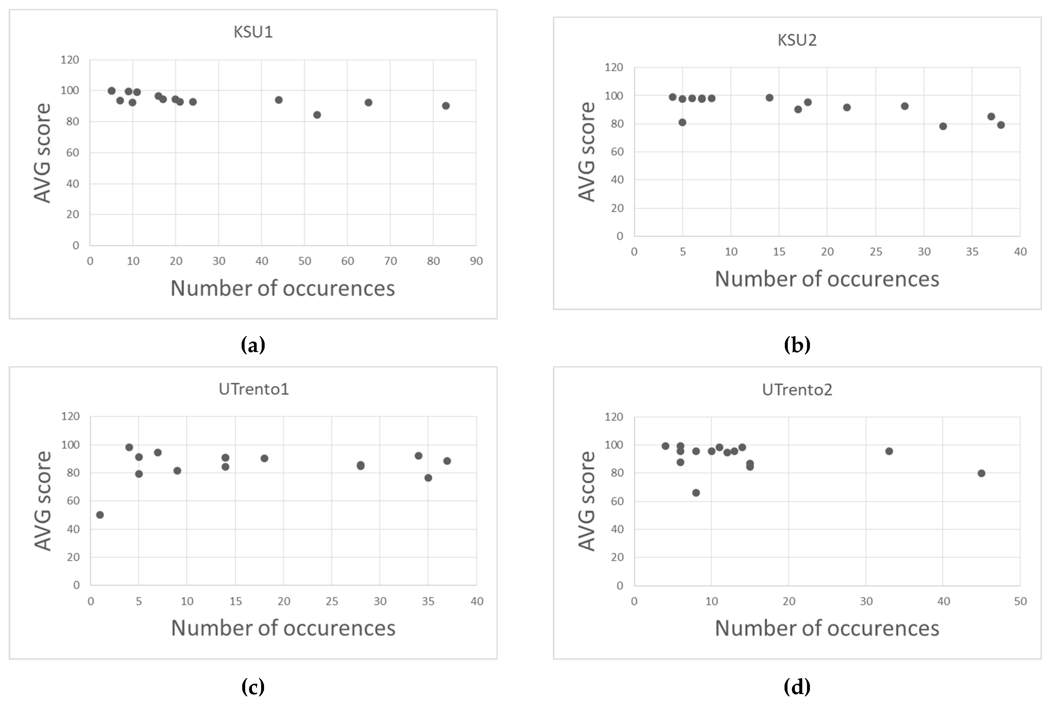
-	AVG	88.31	-	AVG	92.44

presents the AVG scores achieved by Model 3 for all object classes and all datasets where the CONV2D layer size is fixed to 256 and $T_p=0.3$. In general, some objects are harder to recognize because of their low occurrence number in the datasets. For example, if we look at object 10 (class of people) in the Utrento1 dataset, we can see that it appears only once in the whole dataset. This explains the recognition rate of 50% achieved, because with only one example of this object, the network achieves a rate equal to random guessing. In the Utrento2 dataset, the same class of objects (the “people” object) appeared slightly more often (8 times) and was recognized 66% of the time only. Therefore, another reason for the low score for this object class is that it is a complex object with high variability, making it difficult to detect without a large number of training samples.

However, for other objects and despite the low number of occurrence for some of them, their recognition rate is mostly above 80% (see Figure 14). This is actually due to the fact that most of the objects are man-made and have low intra-class variability in their appearance, especially with the same dataset coming from the same building. This is also explained by the power of the pre-trained CNN to transfer knowledge from an auxiliary domain with a large dataset to another domain with a smaller dataset.

In the UTrento datasets, there are large barrel geometric distortions of the images. In our opinion, this partly explains the lower AVG scores achieved on these datasets compared to the KSU datasets. For example, in Figure 9, one can observe that the “Board” objects are sometimes located on the edges/corners of the image and hence become distorted, making them harder for the network to recognize. This partly explains the relatively lower AVG score achieved for this object, namely 85.90% and 79.96% in the UTrento1 and UTrento2 dataset, respectively, despite their high number of occurrences.

5. Conclusions

In this paper, we have presented an efficient deep learning method for image multi-labeling. This method is a module belonging to a larger system for helping the visually impaired to navigate his environment and recognize objects therein. The system makes the VI person aware of the presence/absence of a given set of objects in his environment. Our solution is based on a light-weight pre-trained CNN called SqueezeNet. We developed an improved version of the SqueezeNet by resetting the weights of the last convolutional layer to new random values, changing the activation function from a ReLU to LeakyReLU, and adding a BatchNormalization layer. Next, using a fine-tuning approach, we successfully trained the proposed deep CNN on four image multi-labeling datasets. Experimental results have shown the effectiveness of our proposed deep CNN, because it has provided significant improvements over the state of the art and has reduced the computational time per image.

Upon inspection of Figure 10, we can observe that the objects have a different number of occurrences in each dataset. This creates a class imbalance problem that negatively affects any classification method. Thus, one future direction of research in order to improve the classification results is to address the class imbalance problem. One way to do this is through augmentation techniques to increase samples in the infrequent classes. Another direction is the use of an ensemble of deep classifiers, where each one is responsible for learning to detect a set of objects that are more balanced in terms of their frequency of occurrence. An intelligent fusion technique could then be used to merge the results of the classifier ensemble.