A Parametric Identification Method of Human Gait Differences and its Application in Rehabilitation

Abstract

In order to understand the regularity of human motion, characteristic description is widely used in gait analysis. For completely expressing gait information and providing more concise indicators, parametric description is also particularly significant as a means of analysis. Therefore, in this paper, the mathematical models of gait curves based on the generalized extension-Bézier curve were investigated, of which the shape parameters were used as individual gait characteristics to distinguish whether the gait is normal or not and to assist in judging rehabilitation. To evaluate the models, angle data from three joints (hip, knee, and ankle) were recorded with motion capture system when participants (10 healthy males and 6 male patients with ankle fracture) were walking at comfortable velocity along a walkway. Then, the shape parameters of each subject were obtained by applying the mathematical models, and the parameter range of the normal group was further summarized. Through comparison, it could be found that most shape parameters of patients exceed the normal ranges in varying degrees, and are concentrated on specific parameters. The results can not only help to judge the recovery stages of patients but also figure out the corresponding abnormal postures, so as to provide guidance for rehabilitation training.

1. Introduction

Gait is the external behavior characteristics of human walking based on the structure and function of the human body and nervous system. When walking naturally, the gait of lower limbs shows strong periodic regularity [1]. Many studies have proved that people in good condition have similar gait characteristics while some people with disorders show obvious differences compared to them, so the analysis of gait characteristics has gained increasing attention at present [2,3,4,5].

Gait analysis, one of the most commonly used methods to explore gait characteristics, plays a vital role in clinical practice [6]. It mainly divides gait properties into four categories, which are temporal and spatial data (time and distance variables), kinematics (joint motions), kinetics (joint moments, ground reaction forces, etc.), and bioelectrical data (muscle forces and electromyography signals), providing an objective measuring instrument of the subject’s functional level. There are many related works for gait analysis, including computer simulation of normal human gait, gait modelling and simulation based on anatomy, simulation based on neural networks, and automatic gait recognition, etc. [7,8,9,10,11]. In the methods of summarizing gait kinematics data, the most widely used approach is applying statistics to conduct a comprehensive gait analysis by using a motion capture system. In current studies, different ages, genders, walking speeds, etc. are the factors influencing the variety of gait parameters. So, some researchers have summarized the ‘reference ranges’ of gait parameters of healthy individuals under a certain condition by statistics, such as for stride time, joint range of motion, joint adduction moment, and so on [12,13,14,15]. Several reporters focused on the differences of gait parameters between normal people and patients (e.g., cerebral palsy, knee osteoarthritis, etc.) as a valid basis for distinguishing different types of diseases [16,17,18,19,20]. An increasing number of investigations have begun to choose a particular type of patient, conducting more comprehensive assessment through all kinds of gait parameters [21,22,23]. As a result, the gait characteristics of patients have been constantly improved and enriched in academic research; the pathological features of diseases are also well understood and have been mastered in medical care in a data-orienting way, thus providing a more complete basis for diagnosis, gait training [24], and prosthesis design. However, gait analysis principally tries to reflect the overall regularity of a large number of sample statistics while reducing the characteristics of individual differences, which is one inevitable limitation. Besides, there are too many evaluation indexes of gait parameters for characteristics description, and parameters that are more simple and concise for estimation are always required in medical research [25]. In addition, people’s living system has stepped into an in-depth development stage. It has significant values not only for understanding the laws of human motion but also for researching the mathematical model of gait in this information age [26].

There has been a growing awareness that the shape of gait curves during walking can greatly give expressions of the characteristics and structure of gait data. Although various people present very similar situations to the whole curve shape for the same kind of gait feature, differences still exist between them. Therefore, gait curves also contain important information, such as the so-called generality and individuality of the characteristics. On this basis, the study of gait parameter characteristics can be transformed into the study of curve shape characteristics, namely, the parameterization of the gait curve shape. Bézier and NURBS (Non-Uniform Rational B-Splines) are the traditional parametric curves [27,28], and their applications related to gait analysis are most common in the aspects of robot motions and gait recognition [29,30]. They mainly describe the overall shape of curves, and cannot express the differences between similar curves in depth. In recent years, scholars have proposed a series of methods for improving this shortcoming by introducing weight factors [31,32,33,34,35,36], so as to modify the local shapes of curves and reflect the personality characteristics. In [37], a shape-adjustable generalized Bézier curve with high degree (a curve of degree n with n local shape parameters) was presented. This curve can explain the whole shape of a group of curves through control points, and adjust the local shapes of each curve by altering shape parameter values, so that the differences between the curves can be displayed by the differences of shape parameters. The authors of [38] illustrated a generalized extension-Bézier curve (a curve of degree n with n − 1 local shape parameters, GE-Bézier curve for short), which has fewer parameters compared with the one mentioned above. Furthermore, the better correspondence between parameters and local shapes of the curves could be expressed as well. However, these curves were more concerned with mathematical theory, and a few of them (such as cubic extension-Bézier and cubic quasi -Bézier) were just applied to the design of car curves and headlights [39,40]. Therefore, a novel approach is applying the new parametric curve in gait analysis.

The overarching goal in this paper was to investigate the mathematical models of lower extremity gait curves based on the characteristics of the GE-Bézier curve, and to take shape parameters as individual gait characteristics. We hypothesized that the ranges of shape parameters of healthy people represented the whole normal gait pattern while those of patients with lower limb injury in different rehabilitation periods should be out of the ranges in various degrees, so as to evaluate the rehabilitation effects. Due to the corresponding relationship between the shape parameters and the local shapes of the curves, it can also assist in judging the walking postures related to abnormal parameters, thus providing effective references for developing rehabilitation training.

2. Methods

2.1. Participants

Ten healthy males between the ages of 20 and 25 years (mean age 23 (1.4) years, mean weight 65.5 (9.6) kg, and mean height 1.73 (0.07) m) volunteered as the normal group for this experiment. All participants were able to ambulate independently with no low extremity disease or sports injury. Another two male patients with a fracture of the right ankle in the second month of rehabilitation, two in the third month, and two in the sixth month were recruited and consented to participate as the patient group. The average age of them was 22.8 (1.3) years, average weight was 68.8 (5.1) kg, and the average height was 1.75 (0.04) m. All subjects provided written informed consent for the experiment.

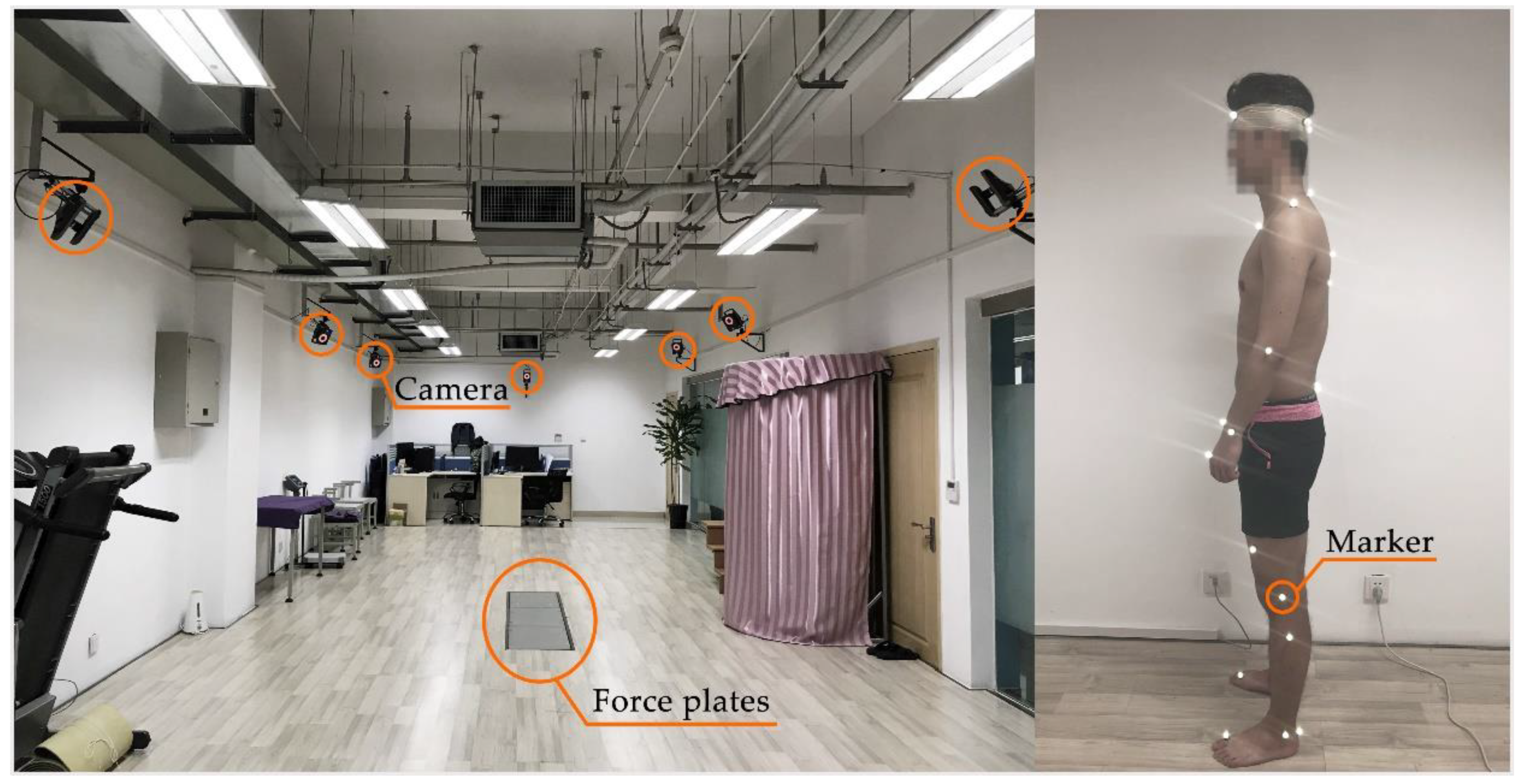
2.2. Data Collection and Processing

The human gait data acquisition experiment was carried out in the Human Gait Capture System Laboratory of Xi’an Jiaotong University, China. All subjects were instructed to walk naturally at a comfortable speed along a walkway for about 5 min and kinematic values of thenlower extremity were obtained through a 10-camera video-based motion capture system (VICON system, Oxford Metrics Limited, UK) operating at 100 Hz. This experiment focused on the right joint rotations (hip, knee, and ankle) in the sagittal plane, i.e., flexion-extension. We hypothesized there would be no difference between the right and left limb. The gait cycle was defined as from the first to second heel strike on the ipsilateral side by the assistance of ground reaction force data recorded using three staggered force platforms, 1500 Hz, embedded in the walkway. The relevant equipment and a participant with markers are shown in Figure 1.

The raw marker trajectories were pre-processed in Vicon Nexus and Mokka, and then the joints angles were calculated using OpenSIM software (SimTK and Stanford University, USA) through the biomechanical gait model (2392) [41].

2.3. Mathematical Model Application

The GE-Bézier curve can be validly applied here to parameterize the periodic curves of lower limb joint angles due to the representability of control points to a global shape of a group of curves and the correspondence between shape parameters and the local shapes of each curve. That is, the distribution range of all curves for one joint could be defined by a group of control points, and then the specific shapes of every curve would be adjusted by shape parameters. Finally, the differences of the shape parameters of curves can be used to distinguish different curves of the same joint.

In this paper, the control points were defined as commonality points. This is because a set of curves can be mathematically described by the identical control points, which determines the distribution range of the overall shape of these curves.

2.3.1. Mathematical Definition of GE-Bézier Curve

For given n + 1 control points P_i∈R^v (i = 0, 1, 2, …, n; v = 2, 3), the curve:

$$r\left(t\right)={\sum }_{i=0}^n{P}_i{G}_{i,n}\left(t\right),t\in \left[0,1\right],$$

(1)

is defined as a generalized-extension Bézier curve (GE-Bézier for short), where the definition of extension Bernstein basis functions $G_{i,n}\left(t\right)$ with parity is constructed.

If n is even:

$$G_{i,n}\left(t\right)=\{\begin{array}{ll}\left(C_{n-1}^i-{\lambda }_{i}t+{\lambda }_{i-1}\left(1-t\right)\right){\left(1-t\right)}^{n-1-i}{t}^i\hfill & i=0,1,\dots ,\frac{n}{2}-1\hfill \\ 2{\lambda }_{i-1}{\left(1-t\right)}^i{t}^i\hfill & i=\frac{n}{2}\hfill \\ \left(C_{n-1}^{i-1}+{\lambda }_{i-1}t-{\lambda }_{i-2}\left(1-t\right)\right){\left(1-t\right)}^{n-i}{t}^{i-1}\hfill & i=\frac{n}{2}+1,\dots ,n\hfill \end{array},$$

(2)

in which the ${\lambda }_i$ is the shape parameter, i = 0, 1, 2, …, n − 2. The parameter ranges are:

$$\{\begin{array}{ll}{\lambda }_{n-2-i},{\lambda }_i\in \left[-C_{n-1}^{i+1},C_{n-1}^i\right]\hfill & i=0,\dots ,\frac{n}{2}-2\hfill \\ {\lambda }_i\in \left[0,C_{n-1}^{\frac{n}{2}-1}\right]\hfill & i=\frac{n}{2}-1\hfill \\ {\lambda }_i=0\hfill & i=-1,n-1\hfill \end{array}.$$

(3)

If n is odd:

$$G_{i,n}\left(t\right)=\{\begin{array}{ll}\left(C_{n-1}^i-{\lambda }_{i}t+{\lambda }_{i-1}\left(1-t\right)\right){\left(1-t\right)}^{n-1-i}{t}^i\hfill & i=0,1,\dots ,\frac{n-1}{2}-1\hfill \\ \left(C_{n-1}^{\left(n-1\right)/2}+{\lambda }_{i-1}\right){\left(1-t\right)}^{n-i}{t}^i\hfill & i=\frac{n-1}{2},\frac{n+1}{2}\hfill \\ \left(C_{n-1}^{i-1}+{\lambda }_{i-1}t-{\lambda }_{i-2}\left(1-t\right)\right){\left(1-t\right)}^{n-i}{t}^{i-1}\hfill & i=\frac{n+1}{2}+1,\dots ,n\hfill \end{array},$$

(4)

in which the ${\lambda }_i$ is the shape parameter, i = 0, 1, 2, …, n − 2. The parameter ranges are:

$$\{\begin{array}{ll}{\lambda }_{n-2-i},{\lambda }_i\in \left[-C_{n-1}^{i+1},C_{n-1}^i\right]\hfill & i=0,1,2,\dots ,\frac{n-1}{2}-2\hfill \\ {\lambda }_i\in \left[C_{n-1}^{\frac{n-1}{2}},C_{n-1}^{\frac{n-3}{2}}\right]\hfill & i=\frac{n-1}{2},\frac{n-3}{2}\hfill \\ {\lambda }_i=0\hfill & i=-1,n-1\hfill \end{array}.$$

(5)

2.3.2. Geometric Properties

The local shapes of the GE-Bézier curve can be adjusted by changing the shape parameters without modifying the control point. The curve will gradually approach the corresponding control point with the increase of the shape parameter value. On the contrary, it will gradually move away, which means that a family of curves with different detail shapes can be generated by Equation (1) with the alteration of the shape parameters after the control points are determined.

For instance, assuming that the whole shape of a curve can be defined by five control points (P₁, …, P₅), then three adjustable shape parameters and their value ranges can be calculated through Equations (1) and (2). Figure 1 depicts how these three shape parameters influenced the local shapes of the curve. Figure 2a shows the overall shape of the curve (in solid line) when all shape parameters were median values, i.e., (${\lambda }_0$, ${\lambda }_1$, ${\lambda }_2$) = (−1, 1.5, −1). When the first shape parameter was the maximum and the minimum of the range of values, and the other two parameters stayed at the median, i.e., (${\lambda }_0$, ${\lambda }_1$, ${\lambda }_2$) = (1, 1.5, −1) and (${\lambda }_0$, ${\lambda }_1$, ${\lambda }_2$) = (−3, 1.5, −1), then, in Figure 2b, the first wave of the curve displayed the highest (in the dash-dotted line), and the lowest (in dashed line), respectively, while the other two waves changed little. In Figure 2c, when the maximum and minimum values were given to the second parameter and the others were intermediate values, for (${\lambda }_0$, ${\lambda }_1$, ${\lambda }_2$) = (−1, 3, −1) in dash-dotted line, for (${\lambda }_0$, ${\lambda }_1$, ${\lambda }_2$) = (−1, 0, −1) in the dashed line, the second wave of the curve appeared from approaching the control point, P₃, to far away from it, and the others remained stable. Similarly, in Figure 2d, only the third parameter was changed, with (${\lambda }_0$, ${\lambda }_1$, ${\lambda }_2$) = (−1, 1.5, 1) in the dash-dotted line, and (${\lambda }_0$, ${\lambda }_1$, ${\lambda }_2$) = (−1, 1.5, −3) in the dashed line. Then, the third wave of the curve went from high to low. In order to acquire the total range of shape adjustment for the curve within the value range of parameters, let (${\lambda }_0$, ${\lambda }_1$, ${\lambda }_2$) = (1, 0, 1) in the dash-dotted line and (${\lambda }_0$, ${\lambda }_1$, ${\lambda }_2$) = (−3, 3, −3) in the dashed line. The grey area in Figure 2e is the whole range of curve shape adjustment under these five control points.

Therefore, (1) in order to ensure that the local shape of the curve has sufficient adjustment ranges when approaching and moving away from corresponding control points, the average curve (with median values of shape parameters) should be chosen to be fitted by Equation (1) to determine the control points’ numbers and coordinates. In this article, it refers to the three average angle curves of joints (hip, knee, and ankle) from the normal group to be fitted. (2) The control points of the normal group are taken as the reference commonality points for other participants, and the ranges of the shape parameters of the normal group are also taken as the normal ranges of the normal gait. In this way, if the shape parameters of other participants belong to the normal ranges under the reference control points, the gait is normal; otherwise, it indicates abnormal gait.

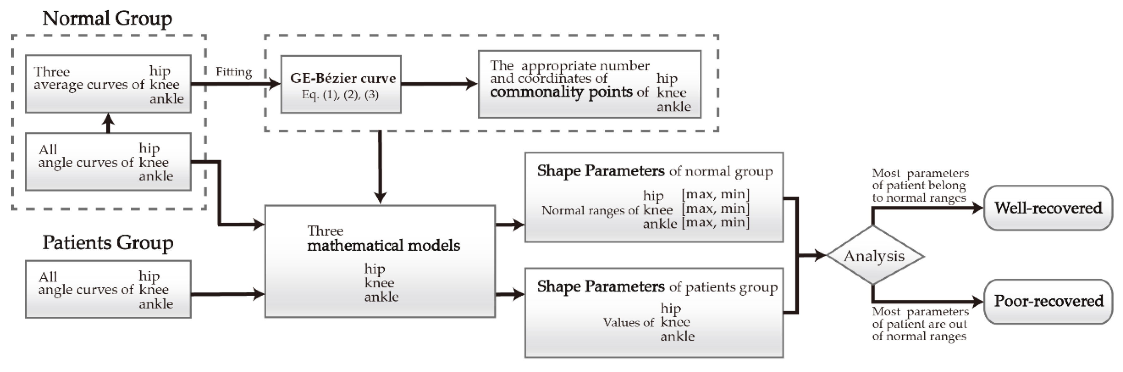
2.4. The Process of Implementation

For the sake of illustrating the whole procedure clearly, the application process of expressing the differences of gait curves by the differences of shape parameters to make a distinction between normal and abnormal gait is shown in Figure 3. For the normal group, the three average gait curves of the participants were initially fitted by the GE-Bézier curve. The appropriate number and the coordinates of commonality points of each average curve was selected and calculated. Then, the mathematical model of each joint was established under the determined commonality points, and the normal ranges of shape parameters (values from maximum to minimum) were summarized through the models. For the patient group, the gait curves were directly fitted by the mathematical models derived from the normal group to calculate the shape parameters of each patient. Then, the shape parameters were analyzed to see whether they belong to the normal ranges. If most shape parameters of well-recovered patients belonged to this range, while most shape parameters of patients with poor recovery were beyond this range, this could indicate that this method can be used to assess rehabilitation status, so its validation is verified.

3. Results

3.1. Normal Group

Figure 4 shows the flexion angle curves (black lines) and their average curves [42] (dark green lines) of the three lower limb joints on the sagittal plane in the normal group. From this figure, the distribution ranges of black lines and the dark green lines are equivalent to the grey area and the solid line in Figure 2e.

Therefore, the dark green lines, the three average curves, were applied to the fitting calculation of Equation (1), then the curve fitting results of different numbers of commonality points are shown in Figure 5 and

Table 1. The three groups of curve fitting results of joints.

Joints	Number of Commonality Points	Number of Shape Parameters	Goodness of Fit
Hip	4	2	0.69
	5	3	1
	6	4	1
Knee	4	2	0.71
	5	3	0.91
	6	4	0.99
Ankle	7	5	0.93
	8	6	0.99
	9	7	1

. Specifically, Figure 5a displays three fitting conditions of four, five, and six commonality points according to the shape characteristics of the hip joint. After comparison, the goodness of fit in five and six commonality points were both 1 with a good fitting degree while the former had not only fewer points but also better correspondence of the numbers between shape parameters and waves than the latter. The average curve of the knee joint was best fitted when controlled by six points according to Table 1. Yet, the correspondence between three waves and four parameters was not clear enough. Although the fitting curve controlled by five commonality points did not fit the original curve completely (see Figure 5b), the proper reflection of the waveform property and the correspondence of three waves to three parameters still expressed the advantages. As for the average curve of the ankle joint, seven parameters exactly corresponded to seven fluctuations when controlled by nine points. Nevertheless, on the principle of minimizing parameters, smaller amplitudes that have little effects on gait feature analysis could be omitted for matching. Through the comparison of the first two fitting curves in Figure 5c, the goodness of fit and the parametric correspondence achieved better satisfaction when controlled by eight points.

The ultimate determined number of commonality points of three joints and the distribution ranges of the curve shapes in the normal group are presented in Figure 6.

Table 2. Coordinates of commonality points of three joints.

Coordinates of Commonality Points
Hip	0.00,30.00	15.30,32.62	63.79,−64.87	73.30,37.28	100.00,27.83
Knee	0.00,4.99	19.31,27.70	57.28,−47.12	69.36,90.93	100.00,3.53
Ankle	0.00,−5.35	8.26,−17.37	17.36,1.62	35.83,−3.41	54.83,17.49	67.63,−43.10	81.35,9.04	100.00,−4.65

exhibits the commonality point coordinates of each group of joint curves. Precisely, when the average curves of the hip and knee were both controlled by five commonality points and three shape parameters, respectively, and the ankle curve was determined by eight commonality points and six shape parameters, they exactly represented the nature of the curves with the least parameters. On the whole, the fitting curve retains the feature of the original waveforms and contains the minimum points and shape parameters, and the local shape corresponding to each point has a sufficient adjustment range.

From this perspective, the mathematical models of three joints were then investigated. For the hip and knee joints, both of their curve shapes could be determined by five commonality points (n = 4), but with different coordinates. Hence, the mathematical models of them are:

$$r\left(t;{\lambda }_0,{\lambda }_1,{\lambda }_2\right)={\sum }_{i=0}^4{P}_i{G}_{i,n}\left(t\right),t\in \left[0,1\right].$$

(6)

Then, Equation (2) is introduced:

$$\{\begin{array}{l}\begin{array}{l}{G}_{0,4}\left(t\right)=\left(1-{\lambda }_{0}t\right){\left(1-t\right)}^3\hfill \\ G_{1,4}\left(t\right)=\left(3-{\lambda }_{1}t+{\lambda }_0\left(1-t\right)\right){\left(1-t\right)}^{2}t\hfill \end{array}\hfill \\ G_{2,4}\left(t\right)=2{\lambda }_1{\left(1-t\right)}^2{t}^2\hfill \\ \begin{array}{l}{G}_{3,4}\left(t\right)=\left(3+{\lambda }_{2}t-{\lambda }_1\left(1-t\right)\right)\left(1-t\right)t^2\hfill \\ G_{4,4}\left(t\right)=\left(1-{\lambda }_2\left(1-t\right)\right)t^3\hfill \end{array}\hfill \end{array}.$$

(7)

So, the three shape parameters and the value ranges of the two joints are ${\lambda }_0$∈[−3, 1], ${\lambda }_1$∈[0, 3], ${\lambda }_2$∈[−3, 1] according to Equation (3).

As for ankle joint, the curve shape of it could be defined by eight commonality points (n = 7), and the model is:

$$r\left(t;{\lambda }_0,{\lambda }_1,{\lambda }_2,{\lambda }_3,{\lambda }_4,{\lambda }_5\right)={\sum }_{i=0}^7{P}_i{G}_{i,n}\left(t\right),t\in \left[0,1\right].$$

(8)

Then, Equation (4) is introduced:

$$\{\begin{array}{c}\begin{array}{l}\begin{array}{l}{G}_{0,7}\left(t\right)=\left(1-{\lambda }_{0}t\right){\left(1-t\right)}^6\hfill \\ G_{1,7}\left(t\right)=\left(6-{\lambda }_{1}t+{\lambda }_0\left(1-t\right)\right){\left(1-t\right)}^{5}t\hfill \end{array}\hfill \\ \begin{array}{l}{G}_{2,7}\left(t\right)=\left(15-{\lambda }_{2}t+{\lambda }_1\left(1-t\right)\right){\left(1-t\right)}^4{t}^2\hfill \\ G_{3,7}\left(t\right)=\left(20+{\lambda }_2\right){\left(1-t\right)}^4{t}^3\hfill \end{array}\hfill \end{array}\\ \begin{array}{l}\begin{array}{l}{G}_{4,7}\left(t\right)=\left(20+{\lambda }_3\right){\left(1-t\right)}^3{t}^4\hfill \\ G_{5,7}\left(t\right)=\left(15+{\lambda }_{4}t-{\lambda }_3\left(1-t\right)\right){\left(1-t\right)}^2{t}^4\hfill \end{array}\hfill \\ \begin{array}{l}{G}_{6,7}\left(t\right)=\left(6+{\lambda }_{5}t-{\lambda }_4\left(1-t\right)\right)\left(1-t\right)t^5\hfill \\ G_{7,7}\left(t\right)=\left(1-{\lambda }_5\left(1-t\right)\right)t^6\hfill \end{array}\hfill \end{array}\end{array}.$$

(9)

The six shape parameters and the ranges of values are ${\lambda }_0$∈[−6, 1], ${\lambda }_1$∈[−15, 6], ${\lambda }_2$∈[−20, 15], ${\lambda }_3$∈[−20, 15], and ${\lambda }_4$∈[−15, 6], ${\lambda }_5$∈[−6, 1] according to Equation (5).

At this point, the curves of 10 healthy subjects from the normal group were substituted into the mathematical models for fitting, and the corresponding shape parameters of each person were calculated.

Table 3. Shape parameters of the normal group of three joints.

Shape Parameters of Normal Group
	Hip			Knee			Ankle
	${\lambda }_0$	${\lambda }_1$	${\lambda }_2$	${\lambda }_0$	${\lambda }_1$	${\lambda }_2$	${\lambda }_0$	${\lambda }_1$	${\lambda }_2$	${\lambda }_3$	${\lambda }_4$	${\lambda }_5$
1	−2.20	0.67	−2.18	−0.55	0.78	−1.24	−0.97 a	−12.37	−5.62	−4.62	−6.67	−2.77
2	−1.94	0.72	−1.13	−2.90 b	0.91	−1.75	−4.57	−13.80 b	6.50 a	−17.75 b	−3.82 a	−5.72 b
3	−1.24	1.81 a	−2.41 b	−2.77	1.32	−2.26	−2.27	−11.92	−16.50	−1.37	−8.02	−0.05 a
4	−2.66 b	0.42 b	−0.54 a	−1.96	0.61 b	−1.77	−5.12	5.58 a	−19.75 b	−2.50	−11.92 b	−2.92
5	0.04 a	1.32	−0.73	0.68 a	1.23 a	−1.13 a	−4.15	−5.10	−6.62	−13.00	−8.55	−4.60
6	−2.18	1.70	−2.26	−1.84	0.66	−2.10	−3.47	−1.57	−19.37	−0.12 a	−4.50	−3.12
7	−2.33	1.14	−2.18	−1.98	0.92	−1.96	−2.02	−6.75	−12.62	−5.62	−10.57	−3.02
8	−1.84	0.73	−2.11	−1.67	0.93	−2.11	−3.65	−11.47	−9.87	−12.25	−7.27	−4.92
9	−2.38	0.61	−2.04	−2.38	0.99	−2.20 b	−2.92	−11.10	−2.37	−15.12	−9.82	−2.85
10	−2.03	0.92	−2.12	−1.96	1.14	−1.80	−5.67 b	−10.65	−7.37	−11.50	−9.45	−4.45
Avg.	−1.88	1.01	−1.77	−1.73	0.95	−1.83	−3.48	−7.89	−9.36	−8.38	−8.06	−3.44

^a The maximum value of parameter, ^b the minimum value of parameter.

lists the shape parameters corresponding to each participant’s curve. Then, the maximum and the minimum values were obtained to summarize the normal ranges of parameters used as normal standards.

3.2. Patient Group

Based on the same commonality points and mathematical models with the normal group, the shape parameters of the patient group were calculated and are displayed in

Table 4. Shape parameters of the patient group of three joints.

Shape Parameters of the Patient Group
	Hip			Knee			Ankle
	${\lambda }_0$	${\lambda }_1$	${\lambda }_2$	${\lambda }_0$	${\lambda }_1$	${\lambda }_2$	${\lambda }_0$	${\lambda }_1$	${\lambda }_2$	${\lambda }_3$	${\lambda }_4$	${\lambda }_5$
A	−2.26	0.02 *	−2.77 *	−2.80	1.08	−2.96 *	−6.00 *	−13.20	1.12	−17.00	−15.00 *	−5.87 *
B	−2.33	0.10 *	−2.84 *	−2.38	1.04	−2.87 *	−6.00 *	−14.32 *	5.62	−15.25	−15.00 *	−5.40
C	−0.44	0.23 *	−2.38	−2.33	0.92	−2.70 *	−4.70	−9.90	−16.87	−5.62	−13.80 *	−3.47
D	−2.10	0.30 *	−2.90 *	−2.56	0.42 *	−1.15	−0.07 *	−14.85 *	−15.12	0.25 *	−11.77	−3.62
E	−1.24	0.61	−0.44 *	−2.11	0.50 *	−2.16	0.07 *	−12.07	−4.62	−14.12	−6.60	−5.60
F	−2.33	1.14	−1.47	−0.87	0.46 *	−1.50	−3.70	−8.55	−18.62	−4.62	−5.92	−5.97 *

* The abnormal parameter beyond the normal ranges.

. It can be seen that the parameters of most subjects were beyond the normal ranges to varying degrees. Figure 7 also shows every gait periodic curve of the patients, which can further explain and verify the characterization of shape parameters. Here, we defined that patients A and B were the ones in the second month of rehabilitation, patients C and D were in the third month, and patients E and F were in the sixth month for convenience.

For the hip joint, the latter two parameters of patients A and B were smaller than the normal range, representing that the waves in the two places were lower than the curve distribution area of the normal group, which was consistent with the results of the red and orange lines in Figure 7a. In the third month of convalescence, only the second parameter of patient C was smaller while the last two parameters of patient D were smaller, indicating that the second wave of patient C and the last two waves of patient D were less than the normal distribution range. Moreover, the parameters’ values showed that the amplitudes of patients C and D were larger and tended to be normal compared to that of patients A and B, which is indicated by the gray and purple lines. In the sixth month of recovery, the parameters of patients E and F were within the normal range, except for the last parameter of patient E, as shown in the pink and blue lines.

For the knee joint, the third parameters of patients A, B, and C, and the second parameters of D, E, and F were all lower than the normal range. It can also be seen from Figure 7b that the third amplitudes of patients A, B, and C presented a state far away from normal gradually, and the second amplitudes of patients D, E, and F were just slightly less than normal. These phenomena revealed that most of the patients with a short recovery period were mainly abnormal in the third parameter.

For the ankle joint, the first, fifth, and sixth parameters of patient A, the first, second, and fifth parameters of patient B, and the fifth parameter of patient C were all smaller. It should be noted that the first and fifth parameters of patients A and B were not only smaller than the normal range but also reached the critical values from Equation (9), indicating that they could not be effectively fitted. For patient D, the first and fourth parameters were larger and the second parameter was smaller. The first parameter of patient E was larger while the sixth parameter of patient F was smaller. Figure 7c also expresses that patients A and B were significantly lower than the normal range at the first and fifth amplitudes corresponding to the abnormal parameters, as seen by the red and orange lines. Patient C (grey line) was slightly lower than the normal value at the fifth amplitude, and the curve of patient D (purple line) tended to the normal ranges. By contrast, the curves of patients E and F (pink and blue lines) in the sixth month of recovery basically belonged to the normal range.

Consequently, the properties of shape parameters were consistent with the data graphics, so the shape parameters can effectively reflect the normal and abnormal gait. Furthermore, the results of the shape parameters’ ranges from the normal group and patient group were very similar with the previous assumptions. The primary abnormal parameters were mainly the second and third parameters of the hip joint, the third parameters of the knee joint, and the first and fifth parameters of the ankle joint.

4. Discussion

4.1. Effects of Shape Parameters in Rehabilitation

According to the abnormal shape parameters of the patient group, besides representing abnormal gait, they have some differences in the excess degrees from normal ranges in different rehabilitation phases, which indicates that parameters could assist in evaluating the recovery status of patients. Furthermore, from the graphical results, the largest differences from the normal distribution areas were the second and third amplitude values for the hip, the third for the knee, and the first and fifth for the ankle. These outcomes were the same with the distributions of the primary abnormal parameters of the three joints, so it could demonstrate that the weights of these primary abnormal parameters here were greater than that of other abnormal parameters.

In line with this idea, it can be considered that when these weighted abnormal parameters exceed the normal ranges, the recovery situation is not ideal; if they belong to the normal ranges while other abnormal parameters slightly exceed the normal ranges, the recovery state can be considered good. Moreover, the higher the abnormal parameters exceed the values, the farther they are away from the normal ranges. With this information, patients with unsatisfactory recovery can be further judged. For the hip joint, patients E and F basically restored normal hip rotation, and the joint function of patient C was basically normal while the hip function of patients A, B, and D still seriously suffered due to the ankle injury. It should be noted that patient D was less influenced than patient B than patient A. For the function of the knee joint, the influence degrees of patients D, E, and F were smaller compared with patients A, B, and C. Furthermore, patient C was less than patient B than patient A. For the ankle joint, the recovery of patients E and F was better than patients C and D while patients A and B were relatively poor in rehabilitation.

All in all, the ankle function of patients A and B was still out of condition since they were in the second month of convalescence, and the knee and hip function were significantly affected. In the third month of rehabilitation, although the ankle function of patients C and D improved, it still mainly influenced the hip joint. By the sixth month of the recovery period, the three joint functions of patients E and F were basically restored to normal.

4.2. Effects of Shape Parameters in Walking Postures

In natural walking, the flexion and extension angles of the hip, knee, and ankle joints of healthy individuals changes harmoniously [43], which is different from that of patients. Since each shape parameter corresponds to a wave of the angle period curve, which is exactly the transformation process of walking posture. The abnormality of shape parameters can then assist in judging the abnormality of walking posture in the gait cycle. For the hip joint, the second and third parameters being smaller than the normal range indicated that maximum extension was not achieved in the stance phase, and the forward flexion was not increased enough in the swing phase. In other words, the hip joint was in a slight forward flexion from terminal stance to terminal swing. For the knee joint, the third smaller parameter corresponds to the failure of the patient’s flexion to increase effectively during the swing phase, presenting that the patient’s activity is limited. For the affected ankle joint, the first and fifth parameters were lower, which corresponded to the limitation of two plantar flexion movements in the whole gait cycle, showing that the patients’ feet were still unable to move freely.

Generally, ankle joint injury had an impact on the normal movement of the lower extremity joints. In order to avoid pain in the affected area or due to psychological factors, the patients used the way of dragging the injured legs to walk, resulting in abnormal movements of the lower limb joints. The explanations above also illustrated= that the shape parameter analysis allowed documentation of the patients’ progress after rehabilitation and identified possible directions to adapt the exercise program.

5. Conclusions

This article proposed a parametric description method of mathematical models based on the GE-Bézier curve for the angle variations of three lower extremity joints in the sagittal plane, which can help to distinguish normal and abnormal gait, and assess the rehabilitation status and walking postures of patients by shape parameters. The main conclusions can be summarized as follows:

• The mathematical models were provided for the gait data of each participant, which not only contain the individual gait personality but also present the general gait regularity. In the models, the gait curve shapes of different participants in the same joint can be controlled by one group of commonality points, and the differences among local details of curves were reflected by different local shape parameters.
• For the normal ranges of shape parameters summarized from the normal group in this paper, they can be used as references for distinguishing normal and abnormal gait. The gait could be considered normal if shape parameters in the patient group belonged to these ranges, and if they were exceeded, especially for parameters with larger weights, the gait tended to be abnormal.
• The excess degrees of abnormal parameters can play a certain role in assisting the evaluation of the recovery status of patients. In this context, the degree of abnormal parameters of patients in the second month recovery period significantly exceeded those in the recovery period of six months, indicating that the former has a poor recovery status to a large extent.
• Shape parameters can help analyze abnormal postures during walking. For the patients with an ankle fracture in this paper, it could be estimated that the flexion movements of three lower joints were limited to various degrees corresponding to the abnormal parameters, and these abnormal gait characteristics can in return provide references for rehabilitation guidance.

In future works, we aim to continue to expand the sample size of the same population and calculate the shape parameters to obtain sufficient data to further support the results of the study. Subjects in other ages and genders will also be recruited and measured to acquire the adjustment ranges of shape parameters and to make the method more adaptable in clinical practice. In addition, for the process of judging whether the gait is normal by shape parameters, the possibility of machine learning can be explored. With the support of sufficient data, more accurate weighted parameters can be calculated through a machine learning algorithm, so that the judgment has more experimental evidences

References

1. Afiah, I.N.; Nakashima, H.; Loh, P.Y.; Muraki, S. An exploratory investigation of changes in gait parameters with age in elderly Japanese women. SpringerPlus 2016, 5, 1069–1083. [Google Scholar] [CrossRef] [PubMed]
2. Hollman, J.H.; McDade, E.M.; Petersen, R.C. Normative spatiotemporal gait parameters in older adults. Gait Posture 2011, 34, 111–118. [Google Scholar] [CrossRef] [PubMed] [Green Version]
3. Patterson, K.K.; Gage, W.H.; Brooks, D.; Black, S.E.; McIlroy, W.E. Changes in gait symmetry and velocity after stroke: A cross-sectional study from weeks to years after stroke. Neurorehabil. Neural Repair 2010, 24, 783–790. [Google Scholar] [CrossRef] [PubMed]
4. Worsley, P.; Whatling, G.; Barrett, D.; Holt, C.; Stokes, M.; Taylor, M. Assessing changes in subjective and objective function from pre- to post-knee arthroplasty using the Cardiff Dempster–Shafer theory classifier. Comput. Methods Biomech. Biomed. Eng. 2016, 19, 418–427. [Google Scholar] [CrossRef] [PubMed]
5. Whittle, M.W. Gait Analysis; Butterworth-Heinemann: London, UK, 1991; pp. 130–173. [Google Scholar]
6. Kirtley, C. Clinical Gait Analysis; Elsevier Health Sciences: Philadelphia, PA, USA, 2006; pp. 5–14. [Google Scholar]
7. Crabtree, C.A.; Higginson, J.S. Modeling neuromuscular effects of ankle foot orthoses (AFOs) in computer simulations of gait. Gait Posture 2009, 29, 65–70. [Google Scholar] [CrossRef] [PubMed]
8. Kim, D.O.; Kang, H.S.; Kim, J.H.; Min, B.G. Virtual anatomy and movement of lower extremities using virtual reality modeling language. J. Digit. Imaging 2000, 13, 238–240. [Google Scholar] [CrossRef]
9. Lapham, A.C.; Bartlett, R.M. The use of artificial intelligence in the analysis of sports performance: A review of applications in human gait analysis and future directions for sports biomechanics. J. Sports Sci. 1995, 13, 229–237. [Google Scholar] [CrossRef]
10. Figueiredo, J.; Santos, C.P.; Moreno, J.C. Automatic recognition of gait patterns in human motor disorders using machine learning: A review. Med. Eng. Phys. 2018, 53, 1–12. [Google Scholar] [CrossRef]
11. Caldas, R.; Mundt, M.; Potthast, W.; Fernando, B.D.L.N.; Markert, B. A systematic review of gait analysis methods based on inertial sensors and adaptive algorithms. Gait Posture 2017, 57, 204–210. [Google Scholar] [CrossRef]
12. Nolan, H.; Evi, V.; Ann, H.; Luc, V.; Vincent, V.R.; Wim, S. Do spatiotemporal parameters and gait variability differ across the lifespan of healthy adults? A systematic review. Gait Posture 2018, 64, 181–190. [Google Scholar]
13. Bae, S.; Armstrong, T.J. A finger motion model for reach and grasp. Int. J Ind. Erg. 2011, 41, 79–89. [Google Scholar] [CrossRef]
14. Stimpson, K.H.; Heitkamp, L.N.; Horne, J.S.; Dean, J.C. Effects of walking speed on the step-by-step control of step width. J. Biomech. 2017, 68, 78–83. [Google Scholar] [CrossRef] [PubMed]
15. Chung, M.J.; Wang, M.J.J. The change of gait parameters during walking at different percentage of preferred walking speed for healthy adults aged 20–60 years. Gait Posture 2010, 31, 131–135. [Google Scholar] [CrossRef] [PubMed]
16. Mutoh, T.; Mutoh, T.; Tsubone, H.; Takada, M.; Doumura, M.; Ihara, M.; Shimomura, H.; Taki, Y.; Ihara, M. Impact of serial gait analyses on long-term outcome of hippotherapy in children and adolescents with cerebral palsy. Complement. Clin. Pract. 2018, 30, 19–23. [Google Scholar] [CrossRef]
17. Debi, R.; Elbaz, A.; Mor, A.; Kahn, G.; Peskin, B.; Beer, Y.; Agar, G.; Morag, G.; Segal, G. Knee osteoarthritis, degenerative meniscal lesion and osteonecrosis of the knee: Can a simple gait test direct us to a better clinical diagnosis. Orthop. Traumatol. Surg. Res. 2017, 103, 603–608. [Google Scholar] [CrossRef]
18. Honda, K.; Sekiguchi, Y.; Muraki, T.; Izumi, S.I. The differences in sagittal plane whole-body angular momentum during gait between patients with hemiparesis and healthy people. J. Biomech. 2019, 86, 204–209. [Google Scholar] [CrossRef]
19. Wren, T.A.L.; Gorton, G.E., III; Õunpuu, S.; Tucker, C.A. Efficacy of clinical gait analysis: A systematic review. Gait Posture 2011, 34, 149–153. [Google Scholar] [CrossRef]
20. Papageorgiou, E.; Nieuwenhuys, A.; Vandekerckhove, I.; Van Campenhout, A.; Ortibus, E.; Desloovere, K. Systematic review on gait classifications in children with cerebral palsy: An update. Gait Posture 2019, 69, 209–223. [Google Scholar] [CrossRef]
21. Elbaz, A.; Mor, A.; Segal, G.; Bar, D.; Monda, M.K.; Kish, B.; Nyska, M.; Palmanovich, E. Lower extremity kinematic profile of gait of patients after ankle fracture: A case-control study. J. Foot Ankle. Surg. 2016, 55, 918–921. [Google Scholar] [CrossRef]
22. Siasios, I.D.; Spanos, S.L.; Kanellopoulos, A.K.; Fotiadou, A.; Pollina, J.; Schneider, D.; Becker, A.; Dimopoulos, V.G.; Fountas, K.N. The role of gait analysis in the evaluation of patients with cervical myelopathy: A literature review study. World Neurosurg. 2017, 101, 275–282. [Google Scholar] [CrossRef]
23. Rucco, R.; Agosti, V.; Jacini, F.; Sorrentino, P.; Varriale, P.; Stefano, M.D.; Milan, G.; Montella, P.; Sorrentino, G. Spatio-temporal and kinematic gait analysis in patients with Frontotemporal dementia and Alzheimer’s disease through 3D motion capture. Gait Posture 2017, 52, 312–317. [Google Scholar] [CrossRef] [PubMed]
24. Goffredo, M.; Iacovelli, C.; Russo, E.F.; Pournajaf, S.; Blasi, C.D.; Galafate, D.; Pellicciari, L.; Agosti, M.; Filoni, S.; Aprile, I.; et al. Stroke Gait Rehabilitation: A Comparison of End-Effector, Overground Exoskeleton, and Conventional Gait Training. Appl. Sci. 2019, 9, 2627. [Google Scholar] [CrossRef]
25. Cimolin, V.; Galli, M. Summary measures for clinical gait analysis: A literature review. Gait Posture 2014, 39, 1005–1010. [Google Scholar] [CrossRef] [PubMed]
26. Zhao, L.; Huang, S.; Xu, Y.; Li, J.; Yu, L. The Movement Model of the Knee Joint during Human Walking. In Proceedings of the IEEE International Conference on Intelligent Human-machine Systems & Cybernetics, Hangzhou, China, 26–27 August 2013. [Google Scholar]
27. Prautzsch, H.; Boehm, W.; Paluszny, M. Bézier and B-Spline Techniques; Springer Science & Business Media: New York, NY, USA, 2002; pp. 9–22. [Google Scholar]
28. Piegl, L.; Tiller, W. The NURBS Book, 2nd ed.; Springer: New York, NY, USA, 1997; pp. 7–101. [Google Scholar]
29. Shen, W.; Chai, C.K. Research on motion optimization for quadruped robot based on swing-leg retraction. Trans. Beijing Inst. Technol. 2018, 38, 1269–1275. (In Chinese) [Google Scholar]
30. Sun, X.R.; Zang, X.Z.; Liu, Y.X.; Lin, Z.K. Dynamic analysis and gait planning of biped robot with underactuated ankle. J. Harbin Univ. Commer. (Nat. Sci.) 2017, 33, 319–323. (In Chinese) [Google Scholar]
31. Guo, Q.W.; Xiong, J.; Zhu, G.Q. Extensions of C-Bézier curves and surfaces. Comput. Eng. Appl. 2009, 45, 170–173. [Google Scholar]
32. Han, X.A.; Huang, X.L.; Ma, Y.C. Shape analysis of cubic trigonometric Bézier curves with a shape parameter. Appl. Math. Comput. 2010, 217, 2527–2533. [Google Scholar] [CrossRef]
33. Qin, X.Q.; Hu, G.; Yang, Y.; Wei, G. Construction of PH splines based on H-Bézier curves. Appl. Math. Comput. 2014, 238, 460–467. [Google Scholar] [CrossRef]
34. Liu, Z.; Chen, X.Y.; Jiang, P. A class of generalized Bézier curves and surfaces with multiple shape parameters. J. Comput.-Aided Des. Comput. Graph. 2010, 22, 838–844. [Google Scholar] [CrossRef]
35. Yang, L.Q.; Zeng, X.M. Bézier curves and surfaces with shape parameter. Int. J. Comput. Math. 2009, 86, 1253–1263. [Google Scholar] [CrossRef]
36. Ri, K. Bézier curves with multi-shape-parameters. J. Zj. Univ. (Sci. Ed.) 2010, 37, 401–405. [Google Scholar]
37. Hu, G. Research on the Theory and Applications of the Generalized Bézier Curves and Surfaces with Shape Parameters. Ph.D. Thesis, Xi’an University of Technology, Xi’an, China, 2016. [Google Scholar]
38. Qin, X.Q.; Hu, G.; Zhang, N.J.; Shen, X.L.; Yang, Y. A novel extension to the polynomial basis functions describing Bezier curves and surfaces of degree n with multiple shape parameters. Appl. Math. Comput. 2013, 223, 1–16. [Google Scholar] [CrossRef]
39. Liu, F.; Ji, X.M.; Gong, L.Q. A CAD modeling method for car form design based on CE-Bézier. In Proceedings of the 11th International Conferences on Computer Graphics, Visualization, Computer Vision and Image Processing (IADIS: 2017), Lisbon, Portugal, 21 July 2017. [Google Scholar]
40. Guo, L.; Ji, X.M.; Hu, G.; Chu, J.J. Car headlight shape design based on cubic Q-Bézier curves. China Mech. Eng. 2013, 24, 1961–1969. (In Chinese) [Google Scholar]
41. Delp, S.L.; Anderson, F.C.; Arnold, A.S.; Loan, P.; Habib, A.; John, C.T.; Guendelman, E.; Thelen, D.G. OpenSim: Open-source software to create and analyze dynamic simulations of movement. IEEE Trans. Biomed. Eng. 2007, 54, 1940–1950. [Google Scholar] [CrossRef] [PubMed]
42. Gao, J.; Cui, Y.H.; Ji, X.M.; Wang, X.P. A method of measuring and analyzing the regularity of human gait. In Proceedings of the International Conference on Mathematics, Modelling, Simulation and Algorithms (MMSA 2018), Chengdu, China, 25–26 March 2018. [Google Scholar]
43. Protopapadaki, A.; Drechsler, W.I.; Cramp, M.C.; Coutts, F.J.; Scott, O.M. Hip, knee, ankle kinematics and kinetics during stair ascent and descent in healthy young individuals. Clin. Biomech. 2007, 22, 203–210. [Google Scholar] [CrossRef]
Figure 1. The experimental scene.
Applsci 09 04581 g001
Figure 2. The relationship between local shapes and three shape parameters of the GE-Bézier curve with five invariant control points (P1, …, P5): (a) The curve with three appropriate waves when the shape parameters were all median values; (b) The first wave changed with the alteration of first shape parameter; (c) The second wave fluctuated if only the second shape parameter was changed; (d) The third wave varied with the third shape parameter; (e) The grey area represents the range of curve shapes within the values of shape parameter ranges.
Applsci 09 04581 g002
Figure 3. The process of investigating the mathematical models of three joints and obtaining the shape parameters of normal group and patient group, thus analyzing whether the patient is well recovered or poor recovered.
Applsci 09 04581 g003
Figure 4. The curves of participants and their average curves of three lower joints in normal ranges: (a) Ten angle curves (black line) and the average curve (dark green line) from the hip joint in one gait cycle; (b) The curves of knee flexion; (c) The ankle joint curves.
Applsci 09 04581 g004
Figure 5. The fitting curves of three groups of commonality points to each joint: (a) The average curve (dark green line) of the hip was fitted through four, five, and six commonality points, respectively. The fitting curve (red line) at five points had the similar matching effect as six points, but with fewer points; (b) The three relationships among the fitting and average curves at four, five, and six points of the knee joint; (c) The average ankle joint curves were fitted by seven, eight, and nine commonality points.
Applsci 09 04581 g005
Figure 6. The determined commonality points and normal ranges of angle curves from the normal group after comparison of the fitting results: (a) Ph1, …, Ph5 connected by a dotted line are the five commonality points of hip joint, which means there were three shape parameters according to the model. The light green area shows the shape distribution of 10 curves and as the hip normal distribution range; (b) There were also five commonality points (Pk1, …, Pk5) and three shape parameters of knee joint curves in one gait cycle; (c) The ankle joint curves were provided with eight commonality (Pa1, …, Pa5) points and six shape parameters.
Applsci 09 04581 g006
Figure 7. The angle curves of patients in three different rehabilitation periods and the comparison with normal ranges: (a) The hip flexion curves of the patient group during one gait cycle; (b) The trend of knee joint angle curves of patients was approximately similar to that of the normal range; (c) Patients A and B showed significant differences in their ankle curves from the normal range compared with other patients.
Applsci 09 04581 g007