Article

Finite Element Modeling of Porous Microstructures With Random Holes of Different-Shapes and -Sizes to Predict Their Effective Elastic Behavior

1
Southwest Jiaotong University, SWJTU-LEEDS Joint School, Chengdu 610031, China
2
Southwest Jiaotong University, School of Mechanical Engineering, Chengdu 610031, China
*
Author to whom correspondence should be addressed.
These two authors contributed equally to this work.
Appl. Sci. 2019, 9(21), 4536; https://doi.org/10.3390/app9214536
Submission received: 22 August 2019 / Revised: 16 October 2019 / Accepted: 22 October 2019 / Published: 25 October 2019
(This article belongs to the Section Materials Science and Engineering)

Abstract

:
Porous materials are promising media for designing medical instruments, drug carriers, and bioimplants because of their excellent biocompatibility, ease of design, and large variation of elastic moduli. In this study, a computational strategy using the finite element method is developed to model the porous microstructures and to predict the relevant elastic moduli considering the actual characteristics of the micropores and their distributions. First, an element-based approach is presented to generate pores of different shapes and sizes according to the experimental observations. Then, a computational scheme to evaluate the effective moduli of macroscopically isotropic porous materials based on their micro-mechanics is introduced. Next, the accuracy of our approach is verified with the analytical solutions of the extreme bounds of the elastic isotropic moduli of a simplified model and with the experimental data available in the literature. Finally, the influence of the shape of pores and their distribution modes are assessed.

1. Introduction

Pores of different shapes and sizes are inevitable constituents of practical engineering materials, such as composites, metals and synthetic materials. They significantly affect the overall elastic properties and the failure mechanism of the material [1,2,3,4,5]. Specifically, they render porous materials more suitable for medical applications [6,7,8,9] because of the high controllability, lightweight, biocompatibility and easy of design. Therefore, it is important to fully understand the influence of pores on the macroscopic material properties and to model them quantitatively to design new materials that meet specific requirements and synthesize novel structures.
So far, experimental testing [6,10] is still the most common approach to investigate the pore effects, but the cost remains high, the process is time-consuming and the data obtained may present a considerable discrepancy. With the rapid development of computer hardware and computational theories, numerical simulation becomes another powerful tool to address practical problems. The finite element method (FEM) is a possible approach to quantitatively evaluate the material properties influenced by defects, like holes, cracks and many other imperfections, in the materials and the large structures in view of its low cost and relatively high efficiency [11,12]. Many pioneering studies concerning this topic [1,2,3,4,5,13,14,15,16,17,18] have been conducted by now, and one critical step is to reconstruct a proper microstructure model of the porous materials. A straightforward way is adopting a commercial package, say Minics or others, to reproduce the true microstructures of porous materials at a specific scale by using the tomographic images generated by the atom-probe tomography [19], electron microscopy [20], X-ray tomography [21], or focused-ion-beam-nonatomography [22]. To be noted, the methods of this kind need a huge number of tomographic images of all directions and different scales so as to construct an accurate description of the porous materials [23] due to the random distribution of pores and their shapes and size variations. Further, the solving process may be very time-consuming and computationally challenging.
The second feasible way is referred to as the equivalent computational methods, which apply certain statistics model to characterize the pore size and distribution and then generate equivalent porous microstructures according to the statistics information, including the pore size, surface-to-volume ratio and so forth, obtained experimentally. To date, these methods are classified into two main categories. The first category assumes that all micro- characteristics of porous microstructures are distributed periodically [16,17,24,25,26], hence, a minimal unit cell [1] is modeled based on the experimental observations and employed to predict the effective macroscopic elastic property of porous materials. Though the modeling process with this method is very efficient and the elastic moduli of materials are evaluated quickly ascribed to the periodic idealization, the overall material property predicted with these models may be quite different from the test data since a limited number of natural porous materials rigidly satisfy this simplification.
The other category of the equivalent computational methods fully considers the randomness of the micro- characteristics of porous materials. In the early years, all pores of porous materials are deemed as regular shapes, say sphere, ellipsoid and so forth, of the same kind [13,14,27] and distributed randomly to facilitate the modeling and analysis. Hereafter, the relative arrangement of pores, i.e., distribution mode, among different randomly-distributed pores, is taken into account in modeling the porous microstructures in Ref. [28,29,30]. Recently, the influence of some more complex and irregular shapes of pores are considered in generating the porous models [15,16,18,31,32,33,34,35], and some particular schemes, say hole forming agent method and space-holder technique, are developed simultaneously to reconstruct the porous model more efficiently. In Ref. [23], a robust numerical approach is developed for generating 3D representative volume element models of bicontinuous nanoporous microstructures using Cahn’s method [36] to generate the Gaussian random field and the sinusoidal wave of fixed wavelength but random in direction and phase. To be noted microstructures of porous materials of practical existence consist of randomly distributed pores of various sizes and different shapes and particularly, the distribution mode of these pores also obviously affects the overall elasticity of materials [13,14,15,16,17,18,31,35]. Hence, this paper aims to elaborate a novel computational strategy for generating porous microstructures accounting for the actual statistical pore-size, -shape and distribution-mode information simultaneously framed within the finite element method. To alleviate the difficulty in discretizing irregularly-shaped pores of various eccentricities from the CAD model and facilitate the pores of different arrangements generation, a generalized explicit mathematical description to characterize the actual pore shapes, which covers the models applied in the open literature [13,14,17,18,27] as special cases, is introduced, and an element-based algorithm is developed to produce porous microstructures of actual porous materials.
This paper is organized as follows. In the next section, the preliminaries of reconstructing porous microstructure considering the influence of pore size, shape and distribution-mode is first introduced and an element-based approach is then developed to generate porous models based on the statistical information observed experimentally. Section 3 is dedicated to introducing a computational scheme to evaluate the overall isotropic moduli of porous materials based on the micro-mechanics. In Section 4, both the experimental and theoretical data from practical materials are used to verify the accuracy of our model and to demonstrate the correctness of our computational scheme. Finally, the relationship between the effective moduli of the porous materials and the pore characteristics is analyzed in detail.

2. Materials in Model and Methods

2.1. Porous Materials under Investigation

Materials with pores are now widely used in material engineering, medicine, and biochemistry, among other fields. Some of the resulting unusual properties have attracted increasing attention in engineering. In medicine, stainless steel, Co-Cr alloys, titanium, and its alloys are the main implant materials used to manufacture artificial joints, bone plates and artificial tooth roots [6,7,8,9,37]. These materials have different pore shapes and sizes, overlapping patterns(distribution modes). Hence, this study aims to elaborate a computational strategy to generate porous models close to the real microstructures, which can lead to a more accurate estimate of the effective elastic moduli of porous materials [15,16,17,18], by taking account of the variation of pore sizes, shapes and the statistics information obtained experimentally.
Titanium and its alloy have been widely used in artificial hip joints, dental implants, and in artificial vertebra joints [12] because of their excellent mechanical properties and good biocompatibility. However, modulus of bones is usually within 10–30 GPa [12] whereas the modulus for titanium and its alloy is typically between 55–117 GPa [12]. This suggests that porous materials are needed to reduce the modulus for better integration with natural bones. Titanium is a poisonous metal that will cause irreversible harm to the human body if it is used as a long term substitute for bones.
Cobalt–chromium (Co–Cr) alloys are the most common alternative for metallic restoration in dental laboratory [38]. They are relatively inexpensive compared to noble alloys and have excellent mechanical properties including a high Young’s modulus, a high corrosion resistance, and a high strength [39,40]. However, these alloys have the highest melting point range, which makes the finishing and other subsequent manufacturing processes difficult as well [39,41].
Porous tantalum is an attractive biomaterial for several clinical applications including hip and knee arthroplasty due to its excellent biocompatibility and good biomaterial properties [42]. In recent years, tantalum and its alloy have been received close attention because they do not cause known disease in humans and are not listed as a possible carcinogen. Additionally, porous tantalum forms a self-passivating surface oxide layer which can help the growth of bones and soft tissue [42].
The three materials presented above have different properties and largely summarize most of the possible pore characteristics in porous materials. They represent different pore shapes, different pore sizes, and different distribution modes.

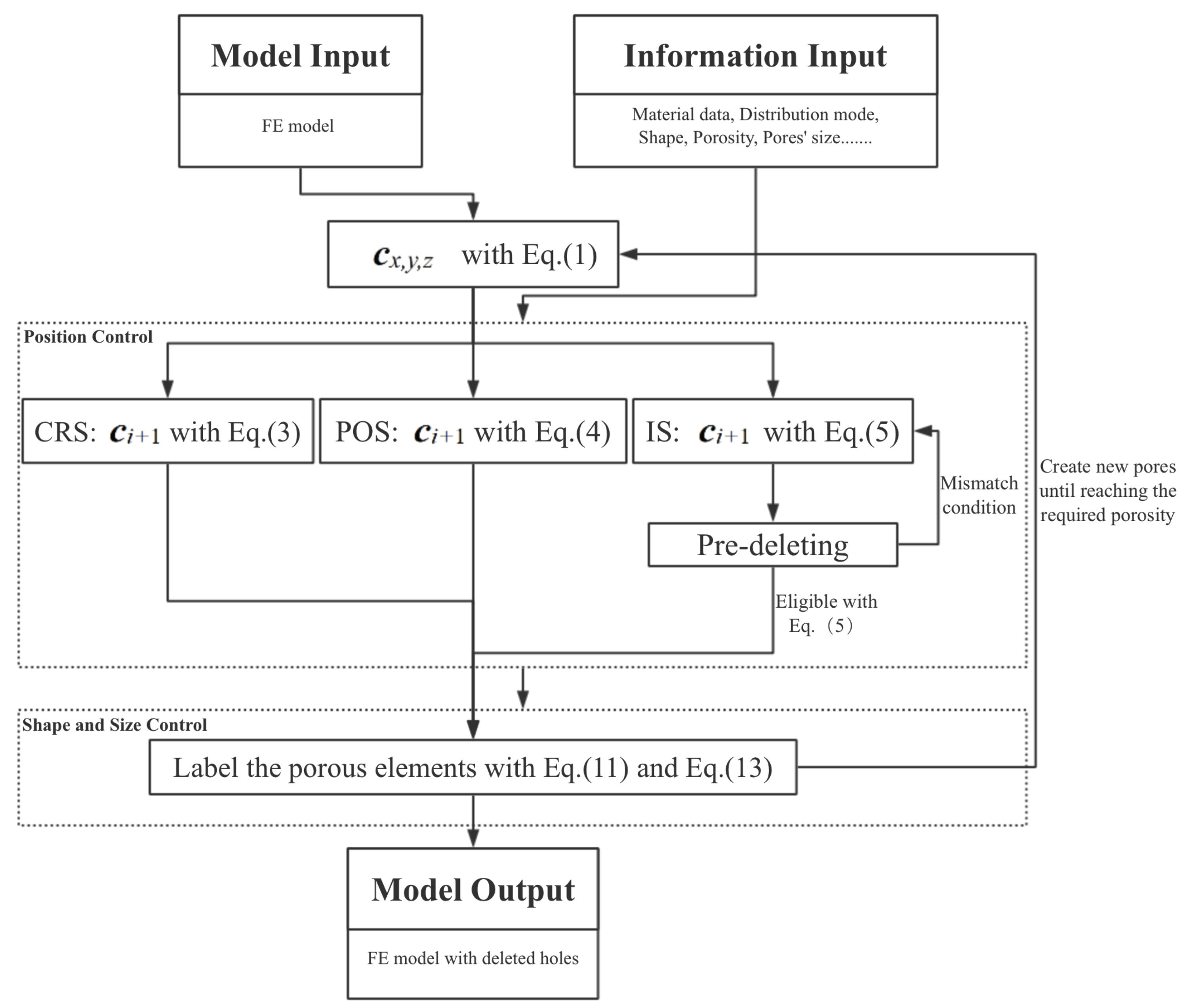
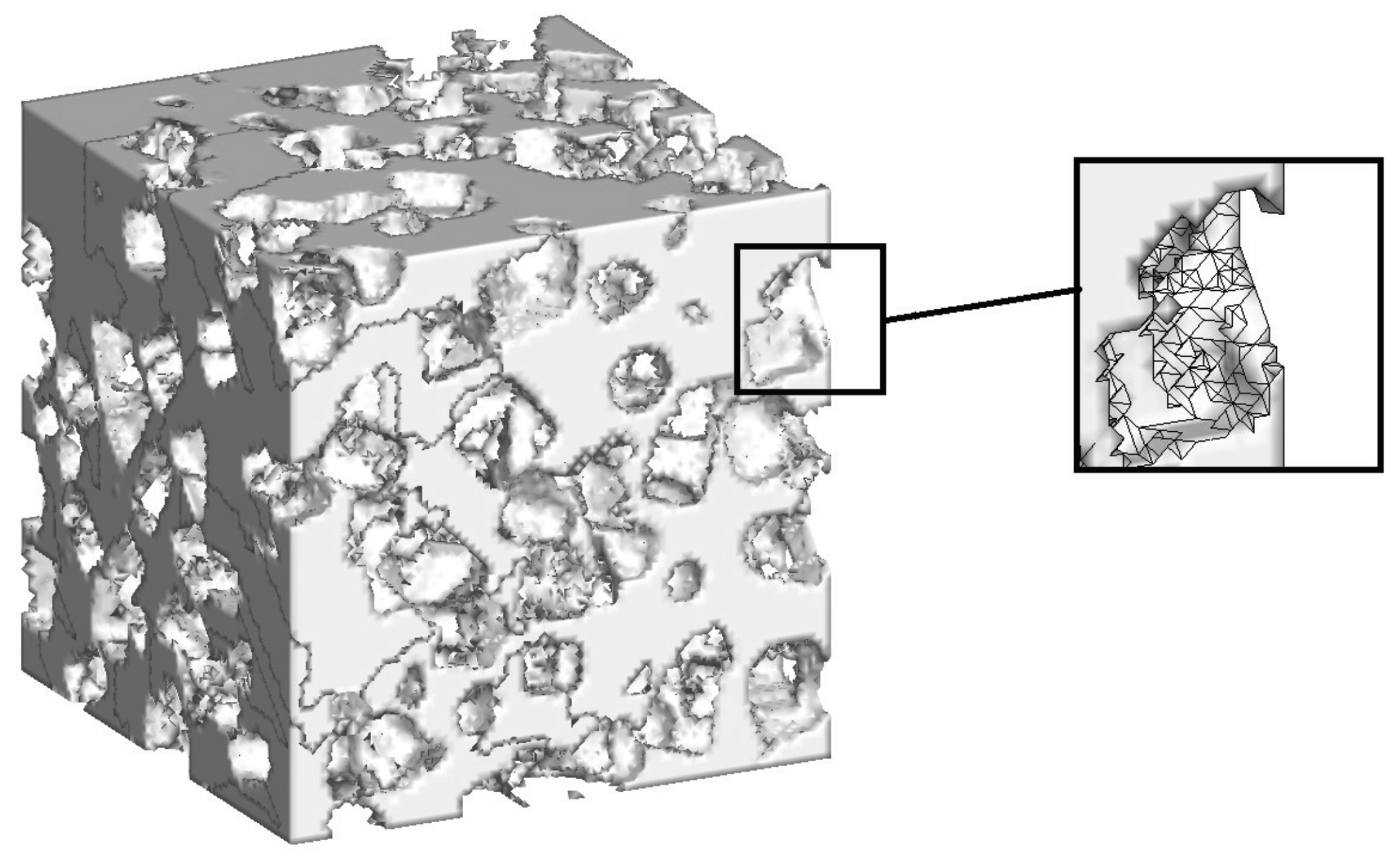
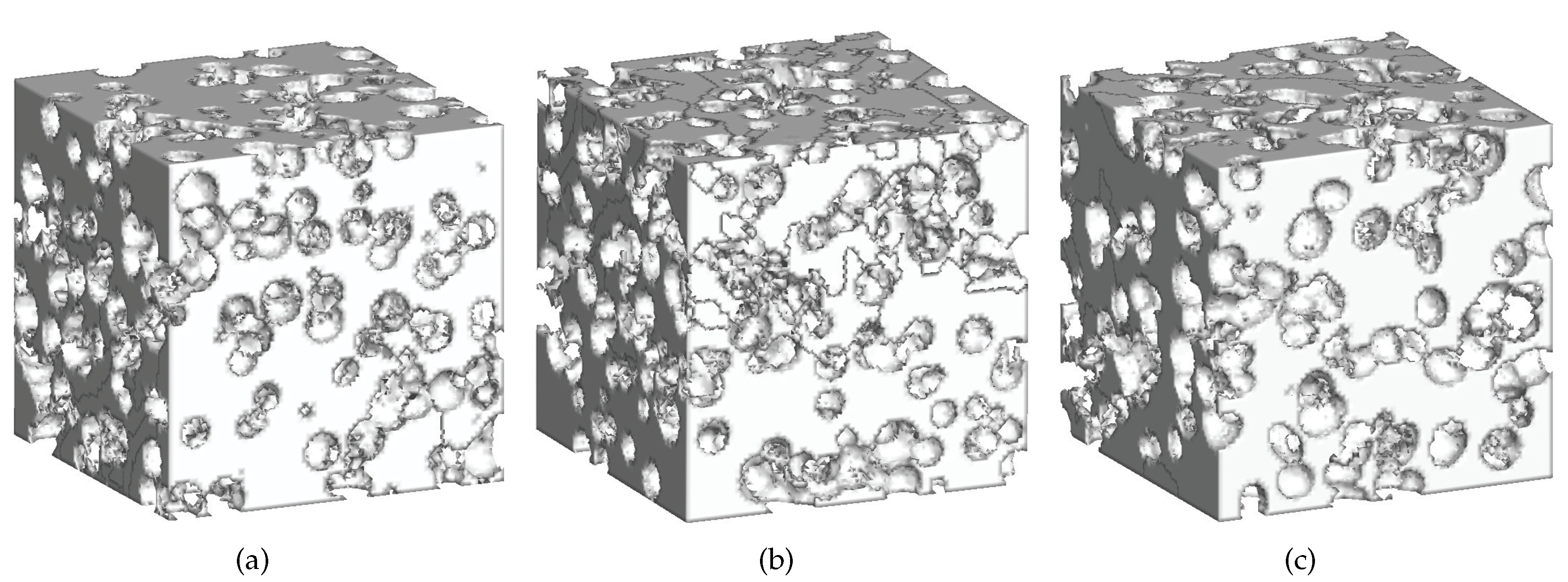
2.2. Generation of Porous Microstructures

The generation of porous model is completed by the following scheme.
The previous general process of forming the porous material numerically is to randomly choose unchanged core points and consider surrounding materials with a very small elasticity to achieve different porosities [30,34]. If any position in the 3D space inside the model boundary can be selected as the pore’s core, the element may not be deleted when the pore radius or the number of elements is small (large volume element). Therefore, we take the center of an element as the generated pore core to ensure that at least one element is deleted in each deletion operation.
Elements with n nodes are numbered in the establishment of 3D finite elements model with the position of each node. Then the position of each element’s center is determined by averaging the coordinates of s nodes:
c x , y , z = i = 1 s x i s , i = 1 s y i s , i = 1 s z i s
where c x , y , z is the position vector of the element’s center, x i , y i , z i are the coordinates of element’s nodes, s equals 4 here because each tetrahedral element adopted contains 4 nodes in our model.
The basic principle of the pore generation process is to delete the element within a given radius from the core element, if spherical pore is required. The expression of nodes, the centers and the relationship between core element and the other element is shown in Figure 1.
The first step is to randomly select an element in the whole model as the core of each pore. This is where the scheme branches off, forming different ways to process different functional requirements, thus implementing the different distribution modes of pores. Based on the previous study, the shape and the distribution of the pores are the two main factors that influence the mechanical properties of porous material [12,30,37,39]. Therefore, we will show how the reconstruction of the porous model is done numerically in different scenarios.

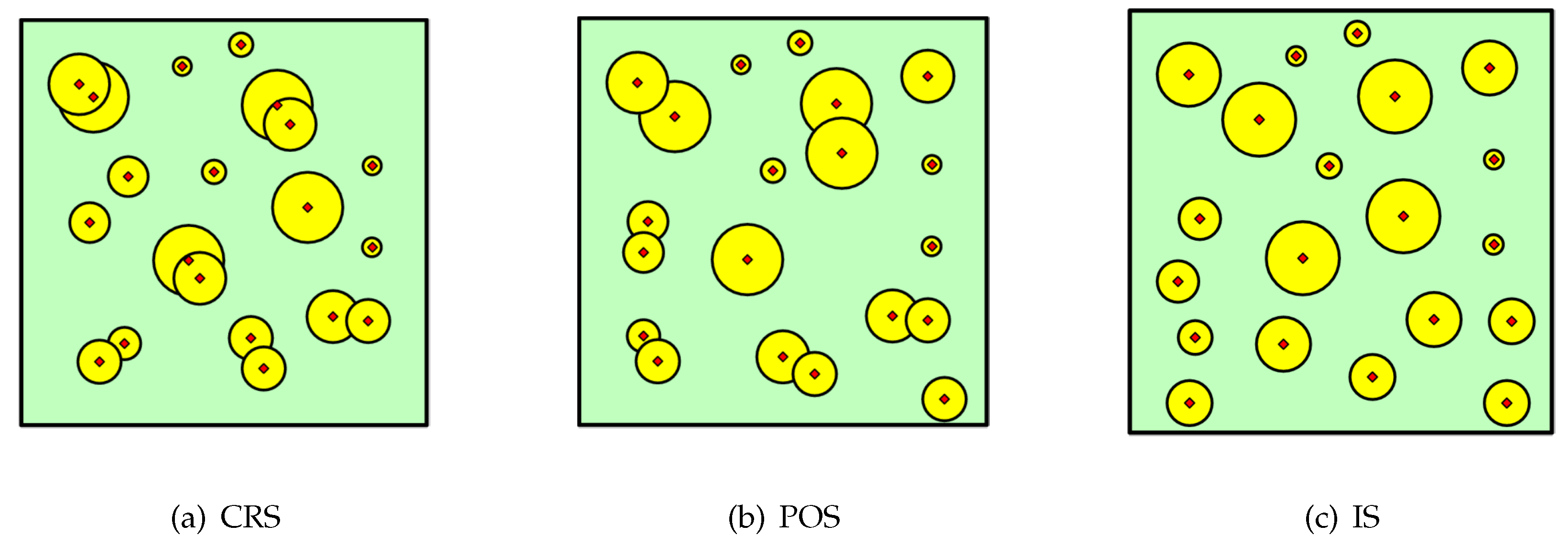
2.2.1. Distribution Modes of Pores

There are three main modes of pores constituting porous materials of different kinds. The difference is shown in the selection of the core element of each pore, and the deletion of the specified elements. Three modes are concluded:
  • Completely random selection (CRS)
  • Partially overlapping selection (POS)
  • Isolated selection (IS)
In CRS, the cores of the pores c i are completely random and the selection spreads all over the model domain Ω within the boundary Ω without any limitation. The program randomly selects an element among all potential candidates to become the core of the pore by generating a random number ξ , which is a real value between 0 and 1: ξ [ 0 , 1 ] . Then the number of the selected element e is:
e = ξ · n t ,
where n t denotes the total number of elements, and is the rounding to integer operator.
When the new selected core c i + 1 is not in one of the element being deleted due to the previous pore generation, the distribution becomes a POS type. In IS, all the pores selected need to be isolated from each other, and their boundaries cannot be overlapped neither.
Numerically speaking, in CRS,
c i + 1 Ω .
In POS,
c i + 1 Ω i .
In IS,
Ω i Ω i + 1 = Ø .

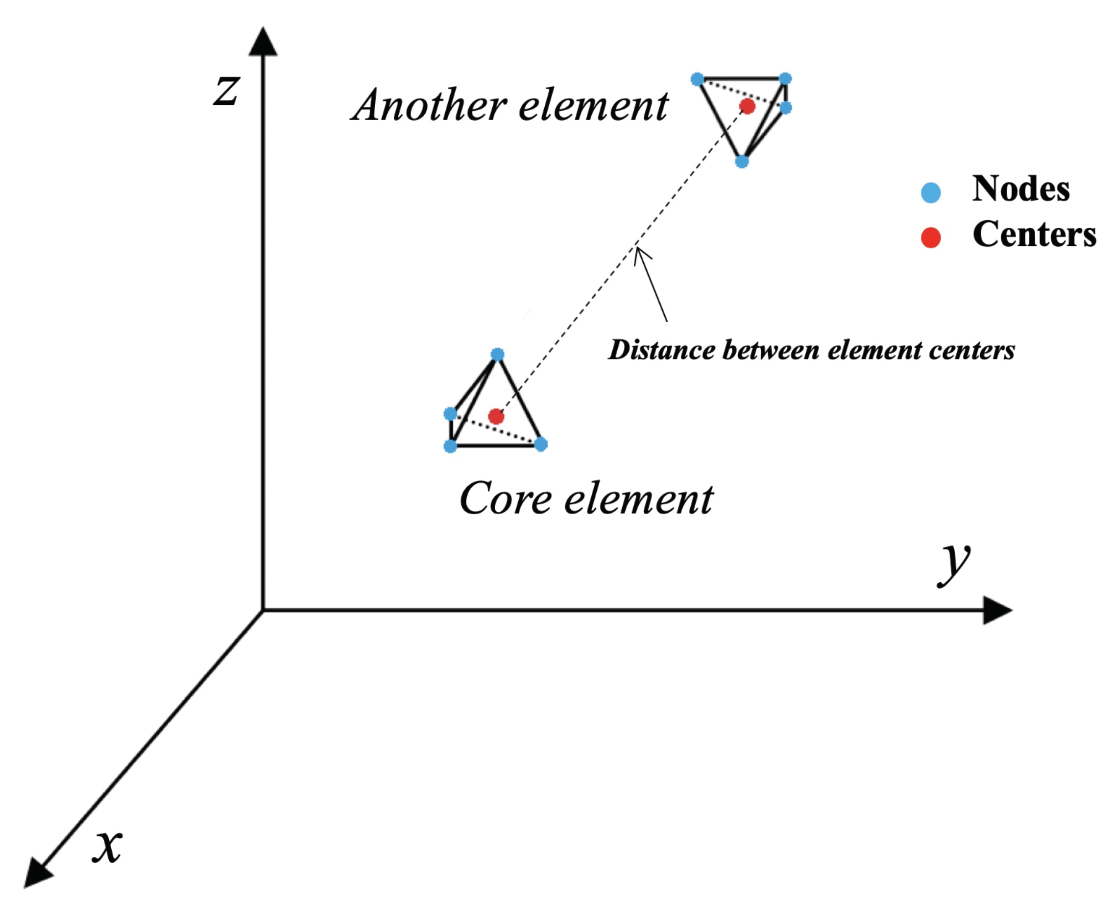
2.2.2. Numerical Simulation of the Pores’ Distribution

The numerical programming to achieve different pore distributions is the key to the simulation of properties of the porous materials. The essential variables are the distance between two cores d and the radii of the two spherical pores r 1 and r 2 .
CRS and POS are very similar to each other. In CRS, the program randomly selects an element among all elements to become the core of the pore by generating random numbers. The selection of the core for the next pore is not limited.
The same process is used in the POS algorithm, but the selective zone of core elements is limited to the elements that are not included in pores that has been previously generated, which translates to:
r 1 < d a n d r 2 < d .
The implementation of the IS algorithm is a little more complicated. There are already some existing strategies to this problem in the previous literature [30]: by extending the distance between two adjacent cores, the two pores could be isolated until the distance between two cores is larger than the sum of the two pore radii, which means:
r 1 + r 2 < d .
There is another way to generate the isolated pores, that results in a better organization. The principle of this algorithm is still based on the random selection of the core element, but all elements that have been deleted as pores previously need to be totally traversed by the program after each selection. If the pore overlaps with the previously formed pore, the selection is abandoned and the next random selection is carried out. If no coincidence element is found, the selection is kept and the pore is generated in accordance with the deleting method.
The schematic 2D figure about the relationship between pores in the three distribution modes is shown in Figure 2. For simplicity, we use the circles to represent pores. Red points represents pores’ cores and the green area represents the solid domain.

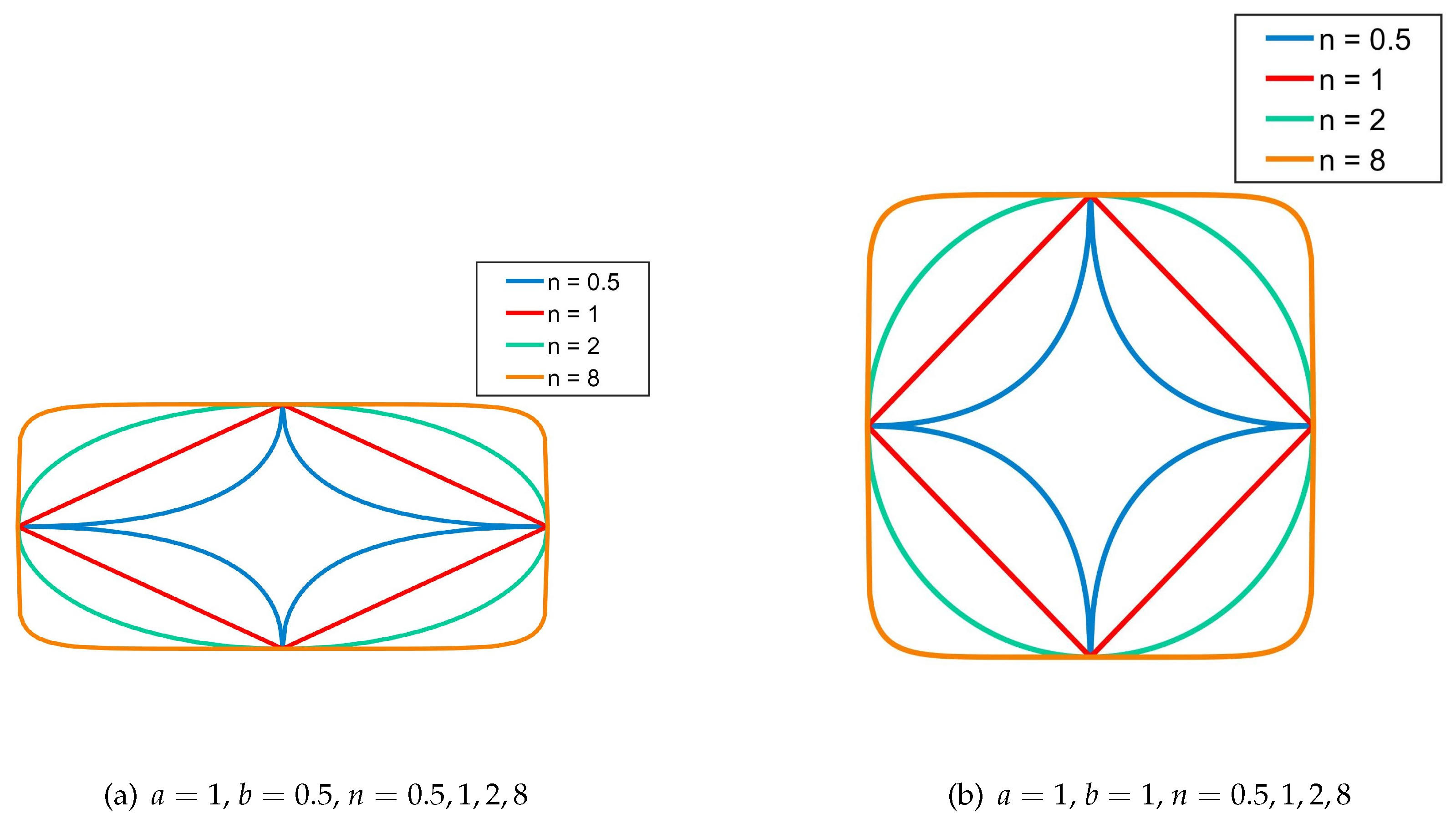
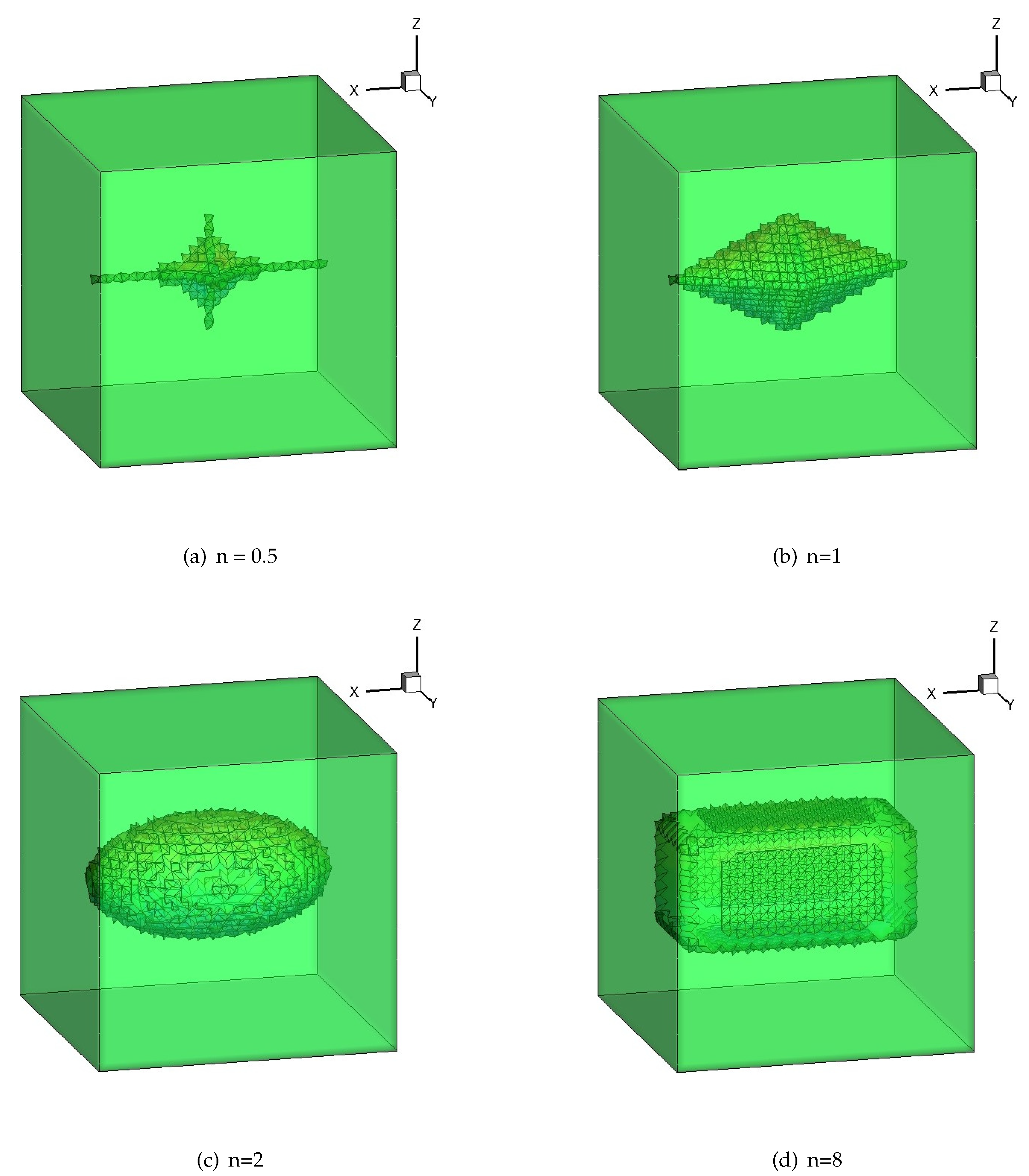
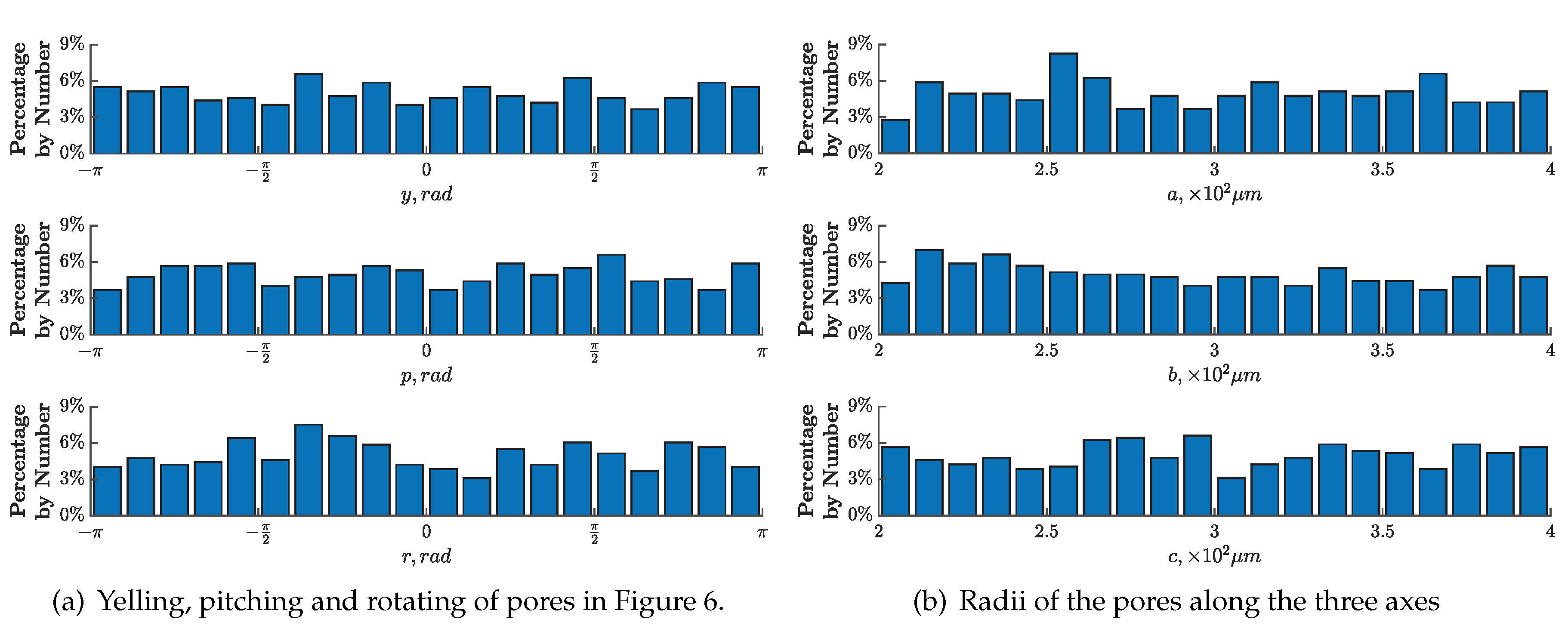
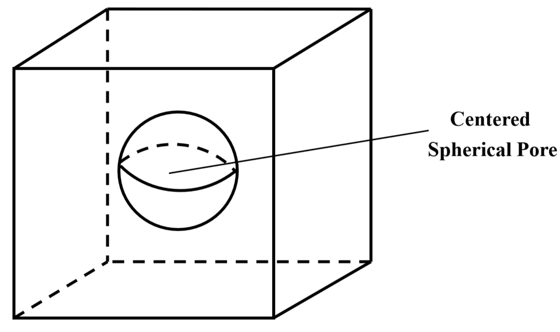
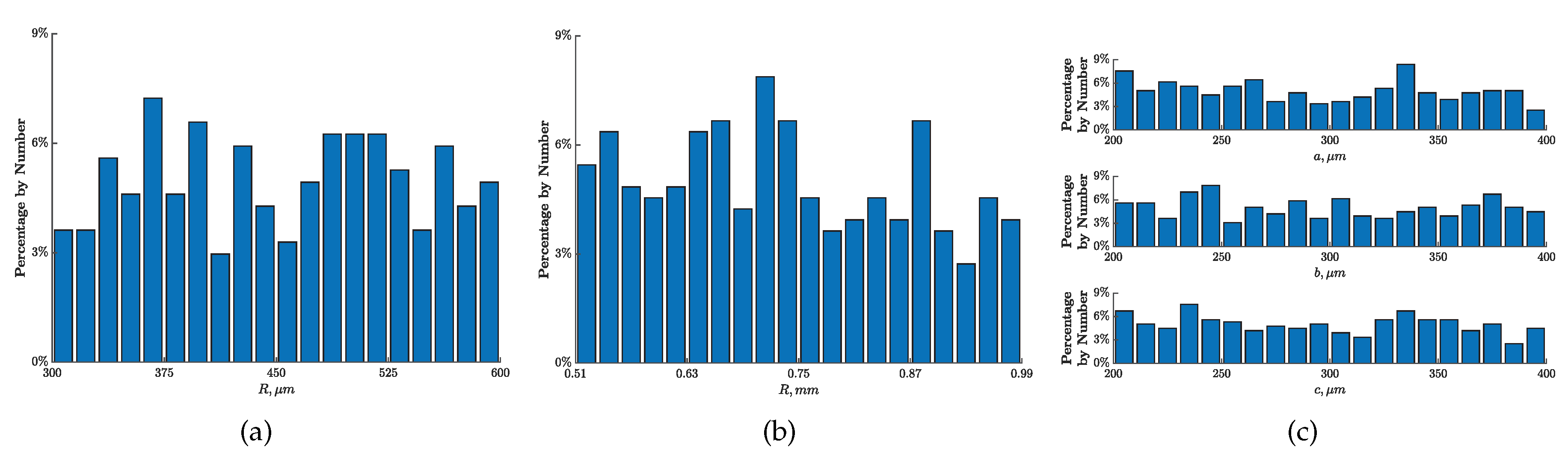
2.2.3. Geometry Equation for Different Pore Shapes and Sizes

The shape of 2D pores can be changed using the following control function.
| x | a n + | y | b n = 1 ,
where a and b are the lengths of the major and minor axis, respectively. By changing the value of n, different shapes can be drawn in 2D plate. The special cases where a = 1 and b = 0.5 , and a = 1 and b = 1 are shown in Figure 3.
To study the property of porous materials, we extend the control function to the 3D domain as:
| x | a n + | y | b n + | z | c n = 1 ,
where a and b are the lengths of the major and minor axis and c represents the length of the pores in z direction. In this case, all parameters needed to describe the pores can be precisely managed to generate different pore shapes. Once the range of the axis length a in the actual material has been obtained: a [ a ̲ , a ¯ ] , a of a pore is determined by:
a = a ̲ + ξ · ( a ¯ a ̲ ) ,
where a ¯ and a ̲ are the upper and lower bounds of a, ξ is a random real number between [ 0 , 1 ] . The values of b and c for each pore are also determined in the same way. This allows random generation of pores of different sizes among the the whole model.
The generation of the pores with those shapes has the following procedure. The elements to be deleted are determined using the distance to the core of each pore in the three axes. In other words, the relative distances from each element to the core in all x, y, and z directions should be obtained first, and the three relative coordinates can be put into the control function.
| x i x c | a n + | y i y c | b n + | z i z c | c n 1 ,
where x i , y i and z i are the coordinates of the center of the detected elements, and x c , y c and z c are the coordinates of the center of the core element. The elements that satisfy Equation (9) are labeled as the area of pores, then the elements will be deleted to form the pore. Then the pore with required height, length, width and shape is obtained by Equation (11) after all the eligible elements are deleted. Figure 4 shows some single pores generated with different index n.
However, this method can only generate pores in one direction, and is not consistent with the random generation approach. Therefore, a rotation equation is used to adjust the direction of the pore by spinning them randomly around three axes in space.
R T = R z R y R x = c o s ( y ) s i n ( y ) 0 s i n ( y ) c o s ( y ) 0 0 0 1 c o s ( p ) 0 s i n ( p ) 0 1 0 s i n ( p ) 0 c o s ( p ) 1 0 0 0 c o s ( r ) s i n ( r ) 0 s i n ( r ) c o s ( r ) ,
where y, p and r donate the yaw, pitch and roll, which controls angles of rotation around z, y, and x axes, respectively. The application of the transformation matrix is described by:
( x i , f x c ) ( y i , f y c ) ( z i , f z c ) T = R T ( x i , o x c ) ( y i , o y c ) ( z i , o z c ) T ,
where x i , f , y i , f ,and z i , f are the coordinates after rotation, x i , 0 , y i , 0 , and z i , 0 are the original coordinates. The foregoing implementation is summarized as a flowchart in Figure 5, and an in-house package is developed using the MATLAB software to perform the computational study in what follows. A porous microstructure generated with the foregoing method is illustrated in Figure 6, and the relevant statistical information of the pores applied are presented in Table 1 and Figure 7. It is noted that the finite elements constituting differently-shaped and -sized pores are preserved in all following computations so as to avoid the numerical difficulties, say isolated elements, boundary condition specification and so forth, and assigned a very small non-negative value for their material parameters (i.e., the Young’s modulus E = 1 . 0 × 10 9 GPa and the Poisson’s ratio v = 0.00001 ). This simplified implementation delivers the same evaluations of the effective moduli of porous media as the method by deleting the aforementioned pore element directly.

3. Local and Effective Elastic Properties

Pores of porous materials are often arbitrarily shaped and randomly distributed in the solid phase, which makes the overall elastic properties difficult to determine analytically or experimentally. The numerical analysis becomes indispensible to this end.
A representative volume element (RVE) is defined if the porous material at the macroscopic scale is assumed to be homogeneous while made up of many repetitive RVEs at the microscopic scale. Then, the overall moduli of porous materials can be determined using the specific boundary excitations together with the local response of an RVE according to the micromechanics.

3.1. Boundary Conditions and Local Governing Equations

Here, we consider a porous material with a domain Ω bounded by its external surface Ω . According to Hills Lemma [43], the displacement boundary condition below is enforced on Ω to determine the overall of the material in question:
u = H x
where H represents the second-order constant tensor and x represents the position vector of the points on Ω . To evaluate the effective properties of the porous material, an RVE model Ω R V E consisting of m pores Ω ( p ) (p = 1, 2, ..., m) is taken out from the porous material Ω of the macroscopic scale.
Here, the material forming the solid phase Ω ( M ) is assumed homogeneous, isotropic and linearly elastic, so that:
σ M = C M ε M ,
where σ M and ε M are the stress and strain tensors over Ω ( M ) , respectively. Symbol C M is the forth-order elastic stiffness tensor of the material forming Ω ( M ) defined by
C M = 3 κ M J + 2 μ M K ,
where J and K are the fourth-order projection operators given as
J = I I / 3 , K = I J .
Above, I and I are the second and fourth-order identity tensors, respectively; κ M and μ M are the bulk and shear moduli of the solid phase. Here, the solid phase is considered as being isotropic so as (i) to obtain the analytical bounds of the effective moduli of a simplified model conveniently and then to validate our approach both theoretically and experimentally, and (ii) to discuss the effect of the pore size and distribution on the overall properties of the true porous material.
According to the displacement boundary condition defined in Equation (14) and because no overlap or separation occurs between the neighbouring RVEs when the external excitations are applied, the displacement boundary condition for an RVE of the microscopic scale is described as:
u RVE = H x .
Thus, the local governing formulas of an RVE are described as:
ε = 1 2 u + u T
σ = C : ε
u ¯ = u RVE ,
where Equations (19) and (20) are applied over the solid phase Ω ( M ) and Equation (21) on Ω R V E .

3.2. Effective Elastic Properties

As indicated by the experimental observations, most porous materials at the macroscopic scale can be considered as nearly linearly isotropic media (see e.g., [6,35,38] and the references therein). Hence, we will focus on developing a numerical scheme to evaluate the overall effective moduli of this particular but very important kind of media in what follows. The overall constitutive equation is thus governed by Hooke’s law:
Σ = C * : E
where Σ and E are the stress and strain tensors at the macroscopic scale, respectively, and are defined by
E = 1 2 V Ω R V E u n M + n M u d S
Σ = 1 2 V Ω R V E ( σ · n M ) x + x ( σ · n M ) d S ,
where n M is the unit normal vector to the boundary Ω R V E of Ω R V E and V is the volume of the Ω R V E . Given the assumption made and the displacement boundary condition in Equation (16), we obtain the relation E = H .
Since the porous material is homogeneous, isotropic and linearly elastic at the macroscopic scale, the effective elastic stiffness is further written as:
C * = 3 κ * J + 2 μ * K
where κ * and μ * are the effective bulk and shear moduli, respectively. To determine κ * and μ * , two conditions are considered individually:
E = I
E = H 1 ,
with t r ( H 1 ) = 0 .
Then, imposing the boundary condition Equation (18) with Equation (26) or Equation (27) on the external surface of the RVE model, and calculate the average stress with Equation (24) numerically, we can finally determine the overall moduli κ * and μ * of the porous material.

4. Validation and Comparison

In this section, our computational method is verified with the extreme bounds of the isotropic elastic moduli of a simplified model together with the experimental data.

4.1. A Benchmark Problem

To verify the computational method presented in the last section, we consider a cubic domain consisting of a spherical pore Ω ( p ) of radius R embedded at the center of the solid cube Ω ( M ) , see Figure 8. The material forming Ω ( M ) is assumed to be linearly elastic and isotropic. Then, the upper bounds of the isotropic elastic moduli of the cubic model in Figure 8 can be determined theoretically when the macrostress excitation [44] is considered, and explicitly expressed as
κ ¯ = 2 4 v m 2 + 3 f ( 4 + 3 f ) v m κ M
μ ¯ = 7 5 v m 7 + 15 f ( 5 + 15 f ) v m μ M .
The lower bounds of the isotropic elastic moduli of the cubic model are obtained when the macrostrain boundary condition [44] is adopted as
κ ̲ = ( 1 + v m ) f 2 ( 1 2 v m ) κ M
μ ̲ = ( 10 v m 8 ) f 7 5 v m μ M ,
where κ ¯ and κ ̲ separately denote the upper and the lower bounds of the bulk modulus, κ M is the bulk modulus of the material forming the solid phase; μ ¯ and μ ̲ are the upper and the lower bounds of the shear modulus, μ M is the shear modulus of the solid phase; f represents the volume fraction of the pore (i.e., porosity); v m is the Poisson’s ratio of the material forming the solid phase and related to the bulk and shear moduli by
v m = 3 κ M 2 μ M 2 ( 3 κ M + μ M ) .
Up to now, the upper and lower bounds of the elastic moduli of the benchmark model in Figure 8 have been obtained and given in Equations (28)–(31).

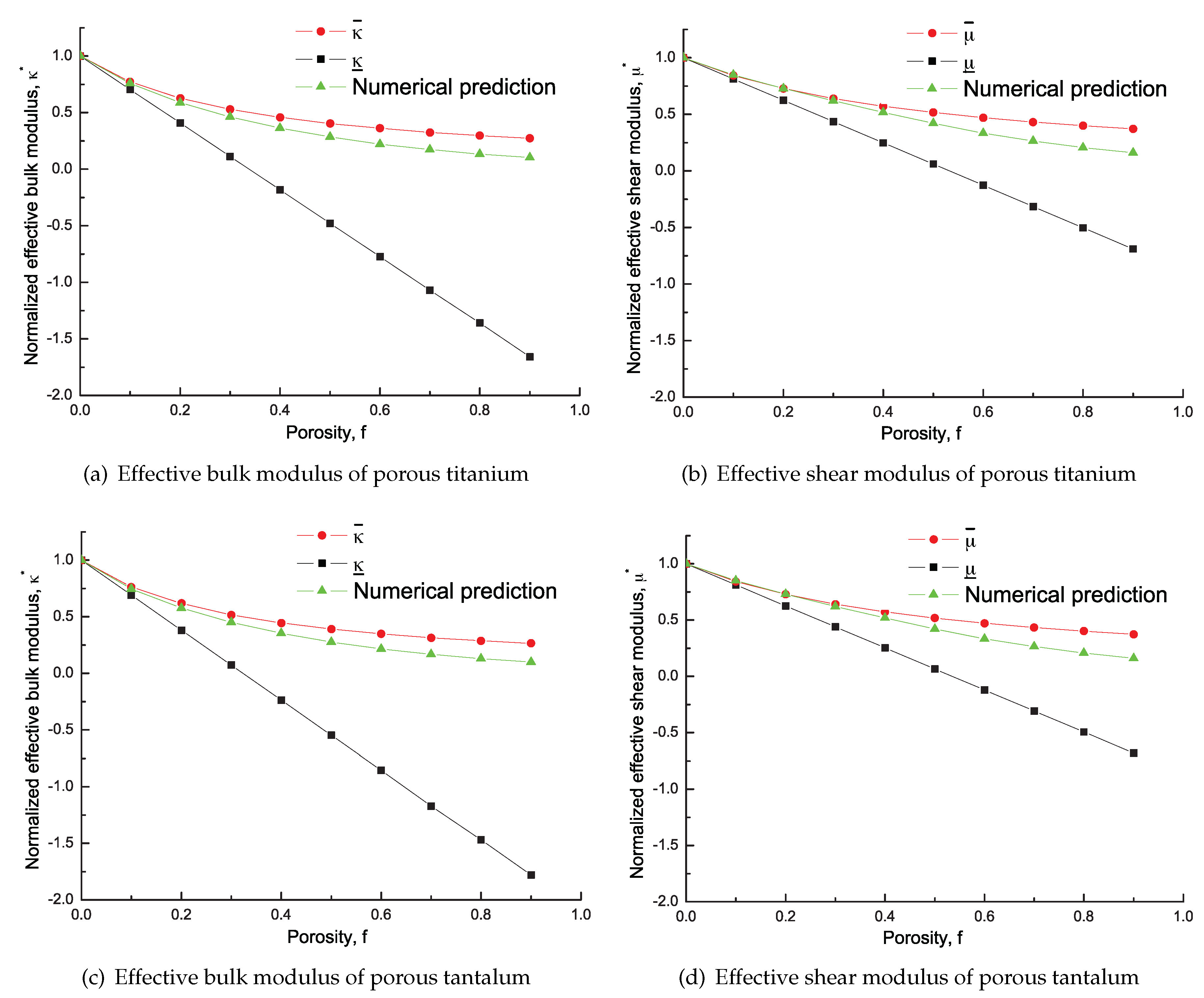
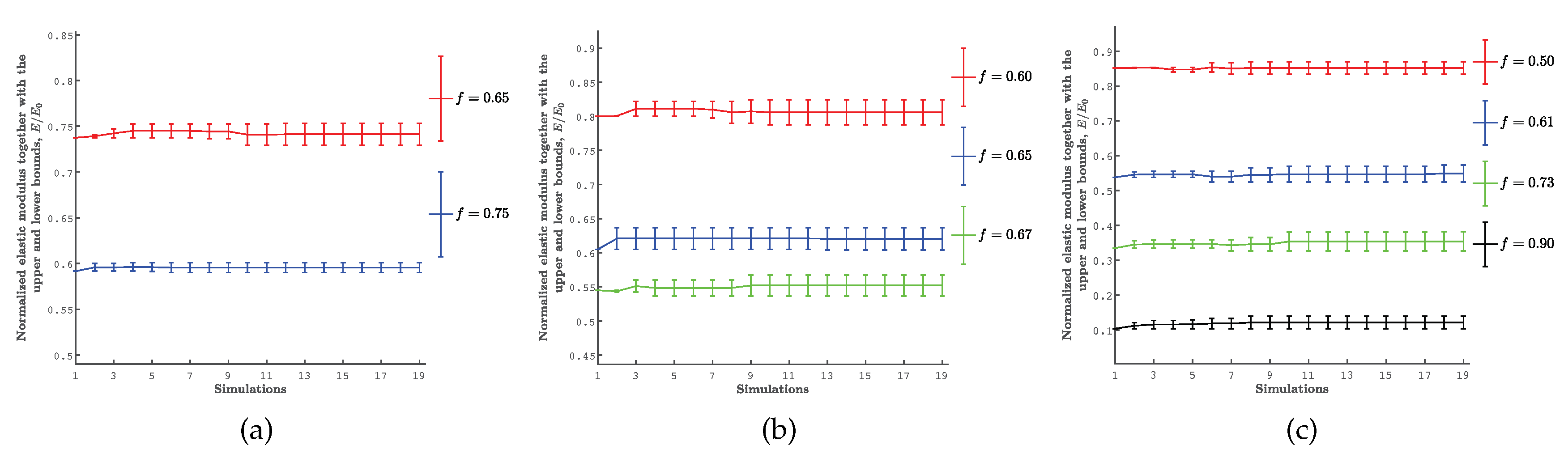
4.2. Verification of the Numerical Predictions with the Theoretical Bounds

To illustrate the correctness of the proposed computational method, the effective elastic moduli of the benchmark model containing differently-sized pores in the last subsection are taken as examples. Since the radii of pores in porous titanium ranges typically from 300 μ m to 600 μ m and those in porous tantalum are usually between 200 μ m and 400 μ m [12,45], the model parameters in Equation (11) are specified as a = b = c [ 300 , 600 ] μ m and n = 2 for the porous titanium and a = b = c [ 200 , 400 ] μ m and n = 2 for the porous tantalum. Besides, the cubic model of side length 1000 μ m is applied. In this study, the 3D domain of each instance is first discretized into ζ × ζ × ζ small cubes and each cube is further discretized into five tetrahedrons. The mesh sensitivity is tested by gradually increasing the ζ value, and a fine enough mesh is adopted to conduct for the following simulations. For the examples in this subsection, each cubic domain in question is meshed by 59 × 59 × 59 × 5 tetrahedral elements. Figure 9 shows the resulting numerical predictions of the isotropic moduli together with the theoretical bounds by Equations (28)–(31). Note that the effective elastic moduli are normalized with respect to the moduli of the solid phase in this study so as to facilitate the visualization of the comparisons.
It is obvious that the numerical predictions are in good agreement with the two bounds when f is small. Particularly, f changes in the range of [ 0 , 0.2 ] , the numerical predication nearly coincides with the upper bounds for both the porous tantalum and the porous titanium. With the increment of f, the range between the upper and lower bounds gets larger and our predictions are strictly in the upper and lower bounds and closer to the upper bounds, which highlights the validity of the numerical predictions by our method. To be noted, the lower bounds by Equations (30) and (31) decrease in a nearly linear manner as f increases and ultimately becomes a negative value, which is infeasible for actual materials.

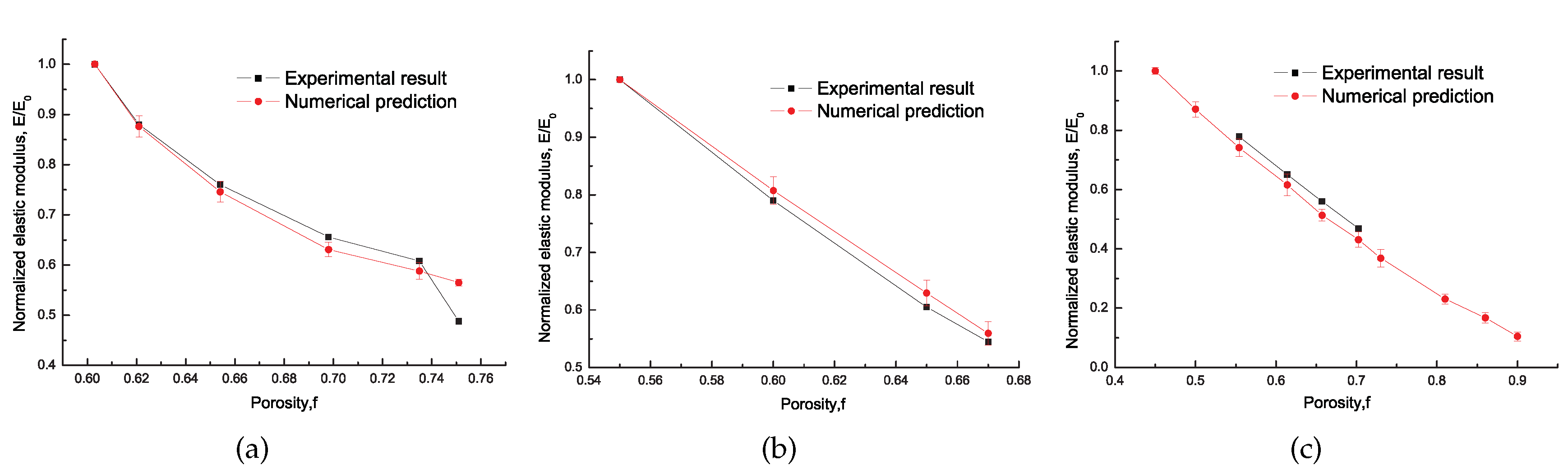
4.3. Comparison of the Numerical Predictions with Experimental Data

In what follows, we shall further verify the computational method developed previously by using the experimental data, and three commonly-applied porous materials, i.e., the porous titanium, the porous CoCrMo alloy and the porous tantalum, are considered in this study. As observed experimentally, the shapes of pores of both the porous titanium and the porous CoCrMo alloys are pretty close to spheres [14,46] (i.e., parameters a = b = c in Equation (11)), and the radius varies from approximate 300 μ m to 600 μ m for porous titanium [12,14] and from 0.51 mm to 0.99 mm for porous CoCrMo alloys [46]. The pores of these two porous media roughly satisfy the POS mode defined in the aforementioned Section. Slightly different from the former two materials, the shape of pores constituting the porous tantalum seems more like an ellipsoid [45], and the radii vary in the range [ 200 , 400 ] μ m, and the relative positions among different pores are supposed to fulfill the CRS relation defined previously [45]. Hence, the model parameters in Equation (11) are set as n = 2 and ( a , b , c ) [ 200 , 400 ] μ m. Sensitivity analysis of the RVE size, as well as the mesh, is then performed by the elastic modulus convergence study, and a cubic domain of side length equal to the value that is fifteen times of the maximum radii of practical pores observed experimentally [45,46], is employed for the verification and meshed with 89 × 89 × 89 × 5 tetrahedral elements so as to generate porous microstructures with the strategy in Section 2 accurately and to obtain the converged numerical evaluations. Figure 10 plots the resulting microstructures of the foregoing porous materials with f = 0.6 , and the relevant morphological parameters adopted are shown in Figure 11. The overall isotropy of the porous RVE models generated has also been examined by using the test approach together with the error indicators ( e E and e κ ) developed in [47] and the necessary and sufficient conditions in [48], and the maximum value of e E and e κ for all instances under consideration is no larger than 6 % . Thus, the macroscopical isotropy of the porous materials consisting of the porous microstructures generated with the computational strategy in this study is approximately guaranteed. The relevant numerically predicted isotropic moduli together with the experimental data in [12,45,46] are visualized in Figure 12. Here, all elastic modulus results are normalized with respect to the elastic modulus associated with the lowest porosity of the porous material.
It is noticed that the elastic moduli of porous media are affected by a number of factors, say the pore size, pore shape, distribution mode and many others, and thus commonly vary from one position to another. Here, the convergence analysis of the number of simulations is carried out to account for the effect ascribed to generating the pore size and position randomly, and Figure 13 visualizes the normalized average elastic moduli together with their upper and lower bounds of the three porous media with different porosities. It is observed that, as the number of simulations increases, the average elastic moduli and the relevant bounds gradually approach to the final results and present so small variations after 12 simulations that it can be considered as being converged for the examples under investigation. Hence, 15 repeated simulations are performed for each porosity of a certain porous medium, which leads to the fact that the effective isotropic moduli predicted numerically in Figure 13 vary in a small range near the relevant mean value. It is observed that both the numerical predictions and the relevant experimental data of all three porous materials under investigation have the same variation as the porosity f increases, and most of the experimental data points are in the range predicted by our computational method. Particularly, the maximum relative error of the numerical predictions and the relevant test data of all instances is no larger than 6 % . The validity of our computational method is thus verified. Note that only the effective moduli of the porous media tested are employed here for validating our computational strategy because the detailed information about the real tomography microstructure of porous media is rarely provided. More investigations will be carried out on comparing the statistical data of the numerically generated porous microstructrues and the real tomography ones and on verifying the fidelity of the generated porous models in our future works.

5. Discussions

As observed by the experimental tests [10,20,45,46], the macroscopic behaviors of porous materials are significantly affected by the porosity, the pore shape and size together with the distribution mode, and the local imperfections. In the following subsections, we shall investigate their influence quantitatively.

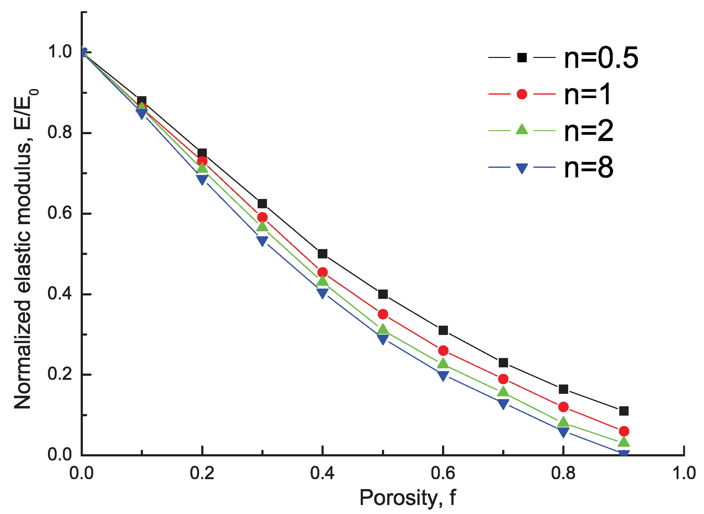
5.1. Shape Effect of Pores

To facilitate the afterward investigation, only the porous tantalum is taken as an illustration and the pore distribution mode is specified as the CRS mode defined in the former section. Equation (11) is adopted to generate pores of different shapes by varying the exponent n. Here, a cubic domain of side length 4000 μ m is employed and meshed by 89 × 89 × 89 × 5 tetrahedral elements to perform the investigation. The model parameters in Equation (11) are specified as a = 400 μ m, b = 200 μ m, c = 200 μ m and n [ 0.5 , 8 ] . The material parameters of the porous tantalum are the same as those in Ref. [46]. The predicted overall isotropic elastic moduli of porous tantalum containing differently-shaped pores are shown in Figure 14. Note that all numerical predictions presented have been normalized with respect to the relevant elastic moduli of the solid material, and only the mean value of the effective moduli are given in the figure for conciseness. Likewise the former subsection, the convergence analysis of the number of simulations is carried out again to ascertain a reasonable value to generate converged evaluations, and 15 repeated simulations are performed for each porosity of the model under consideration here.
It is seen that the effective elastic modulus of porous tantalum decreases rapidly with the increment of the porosity f, and shows obvious dependence on the pore shapes particularly when f is larger than 0.2. Among all shapes of pores under investigation, the model consisting of the pores with n = 0.5 have the maximum elastic modulus as f is a constant. This is attributed to the fact that the shapes of pores greatly affect the connectivity of porous microstructures whose distribution mode of pores conforms to the CRS mode. As n takes a smaller value, more pores have to be generated by the computational method developed so as to guarantee that the porosity of all models are identical. Hence, the pores are distributed more uniformly in these microstructure and the materials of this kind are less prone to generating deformation.

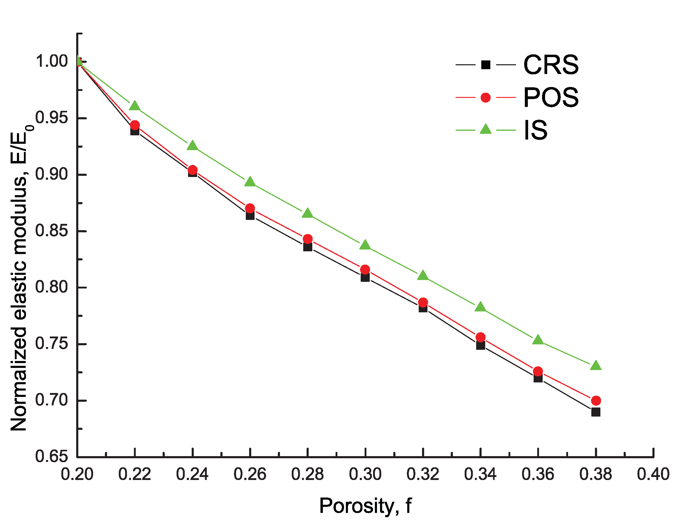
5.2. Distribution Mode Effect of Pores

We shall further examine the influence of the distribution mode of pores on the overall moduli of porous materials. The porous tantalum is taken again as an example and all pores are supposed to be spherical ( n = 2 ) and have the same radius ( a = b = c ) of 400 μ m. The same cubic domain adopted in the last subsection is applied here as well and meshed by 89 × 89 × 89 × 5 tetrahedral elements. All three distribution modes, i.e., CRS, POS and IS, presented in Section 2 are considered for the investigation. Figure 15 shows the mean value of the resulting predictions of the effective modulus normalized by the elastic modulus of the porous material by our computational approach. Similar to the foregoing examples, the convergence analysis of the number of simulations is conducted as well to determine its reasonable value, and 15 repeated simulations are conducted here for each porosity of the model in question. Note that the porosity f under consideration ranges from 0.2 to 0.4 because (i) when f is smaller than 0.2, the distribution modes have negligible effect on the overall modulus of porous materials; ( i i ) when f is larger than 0.4, it is pretty hard to generate a porous microstructure with the IS mode.
From Figure 15, we observe that the effective elastic modulus of the porous material consisting of pores distributed in the POS mode is slightly larger than those of the CRS mode, and these two predictions are obvious smaller than those of the IS mode when the porosity f is identical. Generation of this phenomenon is considered to be the result of the local connectivity of the porous microstructures. Precisely, when the IS distribution mode is considered, all pores constituting the porous microstructure are isolated from each other and distributed more uniformly, hence, the stress induced by the external excitations can be transferred more smoothly in these microstructure compared with the microstructures generated with the other two distribution modes. This particular feature may provide novel ideas for designing porous structures or bioimplants with specific requirements.

6. Conclusions

A computational method was developed in this study to numerically predict the effective elastic modulus of porous materials taking account of the influence of practical pores’ size, shape and distribution mode, and its validity was further demonstrated with both the analytical extreme bounds of the effective modulus of a simplified porous model and the experimental data in the open literature. To be noted, the computational method developed in this work can be easily applied to predict the overall elastic modulus of engineering porous materials by selecting a proper pore model and identifying the relevant model parameters according to the experimental observations and statistic analysis of the pore characteristics. To be noted, though modeling the irregular pores of extremely complex configurations, see e.g., [15,16], are not discussed in this study, our element-based selection method can be easily extended to generate this kind of porous microstructures by combining the level set method, which will be conducted in our future work.
It was found that the overall elastic behavior of porous materials is largely influenced by the pore shape, the pore distribution mode and the porosity. Hence, different measures can be taken to better serve the designing process of the porous materials in actual applications.

Author Contributions

Conceptualization, H.L., S.D. and J.L.; data curation, H.L. and M.W.; formal analysis, Z.Z.; funding acquisition, J.L.; Methodology, H.L. and J.L.; project administration, J.L.; software, H.L. and Y.Y.; supervision, J.L.; validation, S.D. and M.W.; visualization, Z.Z.; writing—original draft, S.D.; writing—review and editing, H.L. and J.L.

Funding

This work was funded by the National Key R & D Program of China (grant number 2017YFB0703200), the National Natural Science Foundation of China (grant number 51972268, 51305362, 11672099, and 51720105005), the Young Scientific Innovation Team of Science and Technology of Sichuan (grant number 2017TD0017), and the Fundamental Research Funds for the Central Universities (grant number 2682016CX024).

Conflicts of Interest

The authors declare no conflict of interest.

Abbreviations

The following abbreviations are used in this manuscript:
FEMFinite element method
RVERepresentative volume element
CRSCompletely random selection
POSPartially overlapping selection
ISIsolated selection

References

  1. Gong, J.F.; Xuan, L.K.; Ying, B.S.; Wang, H. Thermoelastic analysis of functionally graded porous materials with temperature-dependent properties by a staggered finite volume method. Compos. Struct. 2019, 224, 111071. [Google Scholar] [CrossRef]
  2. Martisek, D.; Prochazkova, J. The Enhancement of 3D Scans Depth Resolution Obtained by Confocal Scanning of Porous Materials. Meas. Sci. Rev. 2017, 17, 273–281. [Google Scholar] [CrossRef] [Green Version]
  3. Patel, H.S.; Meher, R. Modelling of Imbibition Phenomena in Fluid Flow through Heterogeneous Inclined Porous Media with different porous materials. Nonlinear Eng. 2017, 6, 263–275. [Google Scholar] [CrossRef]
  4. Wojtacki, K.; Vincent, P.G.; Suquet, P.; Moulinec, H.; Boittin, G. A micromechanical model for the secondary creep of elasto-viscoplastic porous materials with two rate-sensitivity exponents: Application to a mixed oxide fuel. Int. J. Solids Struct. 2019. [Google Scholar] [CrossRef]
  5. Yao, C.; Shao, J.F.; Jiang, Q.H.; Zhou, C.B. A new discrete method for modeling hydraulic fracturing in cohesive porous materials. J. Petrol. Sci. Eng. 2019, 180, 257–267. [Google Scholar] [CrossRef]
  6. Wauthle, R.; van der Stok, J.; Yavari, S.A.; Van Humbeeck, J.; Kruth, J.P.; Zadpoor, A.A.; Weinans, H.; Mulier, M.; Schrooten, J. Additively manufactured porous tantalum implants. Acta Biomater. 2015, 14, 217–225. [Google Scholar] [CrossRef]
  7. Safuan, N.; Sukmana, I.; Kadir, M.R.A.; Noviana, D. The Evaluation of Hydroxyapatite (HA) Coated and Uncoated Porous Tantalum for Biomedical Material Applications. J. Phys. Conf. Ser. 2014, 495, 012023. [Google Scholar] [CrossRef] [Green Version]
  8. Ma, Z.J.; Xie, H.; Wang, B.J.; Wei, X.W.; Zhao, D.W. A novel Tantalum coating on porous SiC used for bone filling material. Mater. Lett. 2016, 179, 166–169. [Google Scholar] [CrossRef]
  9. Levine, B.R.; Sporer, S.; Poggie, R.A.; Della Valle, C.J.; Jacobs, J.J. Experimental and clinical performance of porous tantalum in orthopedic surgery. Biomaterials 2006, 27, 4671–4681. [Google Scholar] [CrossRef]
  10. Wang, S.F.; Wang, C.A.; Sun, J.L.; Zhou, L.Z.; Huang, Y. Fabrication, Structure and Properties of Porous SiC Ceramics with High Porosity and High Strength. Adv. Mater. Res. 2010, 105–106, 608–611. [Google Scholar] [CrossRef]
  11. Sun, W.; Sacks, M.S. Finite element implementation of a generalized Fung-elastic constitutive model for planar soft tissues. Biomech. Model Mech. 2005, 4, 190–199. [Google Scholar] [CrossRef] [PubMed]
  12. Wang, H.B.; Sun, Q.Z. Research on the Influence of Foaming Agent to Porous Titanium. Guangzhou Chem. Ind. 2014, 8, 88–89. (In Chinese) [Google Scholar]
  13. Shen, H.; Oppenheimer, S.M.; Dunand, D.C.; Brinson, L.C. Numerical modeling of pore size and distribution in foamed titanium. Mech. Mater. 2006, 38, 933–944. [Google Scholar] [CrossRef] [Green Version]
  14. Shen, H.; Brinson, L.C. A numerical investigation of porous titanium as orthopedic implant material. Mech. Mater. 2011, 43, 420–430. [Google Scholar] [CrossRef]
  15. Drach, B.; Drach, A.; Tsukrov, I. Prediction of the effective elastic moduli of materials with irregularly-shaped pores based on the pore projected areas. Int. J. Solids Struct. 2014, 51, 2687–2695. [Google Scholar] [CrossRef] [Green Version]
  16. Drach, B.; Tsukrov, I.; Trofimov, A. Comparison of full field and single pore approaches to homogenization of linearly elastic materials with pores of regular and irregular shapes. Int. J. Solids Struct. 2016, 96, 48–63. [Google Scholar] [CrossRef]
  17. Thomas, M.; Basaruddin, K.S.; Safar, M.J.A.; Khan, S.F.; Ibrahim, I. Homogenized properties of porous microstructure: Effect of void shape and arrangement. J. Phys. Conf. Ser. 2017, 908, 012032. [Google Scholar] [CrossRef]
  18. Trofimov, A.; Markov, A.; Abaimov, S.G.; Akhatov, I.; Sevostianov, I. Overall elastic properties of a material containing inhomogeneities of concave shape. Int. J. Eng. Sci. 2018, 132, 30–44. [Google Scholar] [CrossRef]
  19. EI-Zoka, A.A.; Langelier, B.; Botton, G.A.; Newman, R.C. Enhanced analysis of nano-porous gold by atom probe tomography. Mater. Charact. 2017, 128, 269–277. [Google Scholar] [CrossRef]
  20. Rosner, H.; Parida, S.; Kramer, D.; Volkert, C.A.; Weissmuller, J. Reconstructing a nanoporous metal in three dimensions: An electron tomography study of dealloyed gold leaf. Adv. Eng. Mater. 2007, 9, 535–541. [Google Scholar] [CrossRef]
  21. Cho, H.H.; Chen-Wiegart, Y.C.K.; Dunand, D.C. Finite element analysis of mechanical stability of coarsened nanoporous gold. Scr. Mater. 2016, 115, 96–99. [Google Scholar] [CrossRef] [Green Version]
  22. Mangipudi, K.R.; Radisch, V.; Holzer, L.; Volkert, C.A. A FIB-nanotomography method for accurate 3D reconstruction of open nanoporous structures. Ultramicroscopy 2016, 163, 38–47. [Google Scholar] [CrossRef] [PubMed]
  23. Soyarslan, C.; Bargmann, S.; Pradas, M.; Weissmüller, J. 3D stochastic bicontinuous microstructures: Generation, topology and elasticity. Acta Mater. 2018, 149, 326–340. [Google Scholar] [CrossRef]
  24. Weaire, D.; Phelan, R. A counter-example to Kelvin’s conjecture on minimal surfaces. Phil. Mag. Lett. 1994, 69, 107–110. [Google Scholar] [CrossRef]
  25. Gibson, I.J.; Ashby, M.F. The mechanics of three-dimensional cellular materials. Proc. R. Soc. Lond. 1982, 382, 43–59. [Google Scholar] [CrossRef]
  26. Pia, G.; Delogu, F. On the elastic deformation behavior of nanoporous metal foams. Scr. Mater. 2013, 69, 781–784. [Google Scholar] [CrossRef]
  27. Serra, J. Principles-Criteria-Models. In Image Analysis and Mathematical Morphology; Academic Press, Inc.: Orlando, FL, USA, 1983; pp. 3–33. [Google Scholar]
  28. Roberts, A.P.; Garboczi, E.J. Computation of the linear elastic properties of random porous materials with a wide variety of microstructure. Proc. R. Soc. Lond. A 2002, 458, 1033–1054. [Google Scholar] [CrossRef]
  29. Pabst, W.; Gregorova, E. Young’s modulus of isotropic porous materials with spheroidal pores. J. Eur. Ceram. Soc. 2014, 34, 3195–3207. [Google Scholar] [CrossRef]
  30. Guan, K.; Ren, H.T.; Zeng, Q.F.; Wu, J.Q.; Lu, Z.Y.; Rao, P.G.; Cheng, Y.F.; Gong, Z.Y.; Yu, Y.G. Estimating thermal conductivities and elastic moduli of porous ceramics using a new microstructural parameter. J. Eur. Ceram. Soc. 2019, 39, 647–651. [Google Scholar] [CrossRef]
  31. Jauffres, D.; Martin, C.L.; Lichtner, A.; Bordia, R.K. Simulation of the elastic properties of porous ceramics with realistic microstructure. Model. Simul. Mater. Sci. Eng. 2012, 6, 1–18. [Google Scholar] [CrossRef]
  32. Pia, G.; Casnedi, L.; Ionta, M.; Sanna, U. On the elastic deformation properties of porous ceramic materials obtained by pore-forming agent method. Ceram. Int. 2015, 41, 11097–11105. [Google Scholar] [CrossRef]
  33. Ma, J.; Zhang, J.; Li, L.J.; Wriggers, P.; Sahraee, S. Random homogenization analysis for heterogeneous materials with full randomness and correlation in microstructure based on finite element method and Monte-carlo method. Comput. Mech. 2014, 54, 1395–1414. [Google Scholar] [CrossRef]
  34. Niu, W.J.; Gill, S.; Dong, H.B.; Bai, C.G. A two-scale model for predicting elastic properties of porous titanium formed with space-holders. Comp. Mater. Sci. 2010, 50, 172–178. [Google Scholar] [CrossRef]
  35. Li, B.; Wang, B.; Reid, S.R. Effective elastic properties of randomly distributed void models for porous materials. Int. J. Mech. Sci. 2010, 52, 726–732. [Google Scholar] [CrossRef] [Green Version]
  36. Cahn, J.W. Phase separation by spinoal decomposition in isotropic systems. Chem. Phys. 1965, 42, 93–99. [Google Scholar]
  37. Niinomi, M. Introduction. In Metals for Biomedical Devices; Niinomi, M., Ed.; Woodhead Publishing: Cambridge, UK, 2019; p. 3. [Google Scholar]
  38. Kim, H.R.; Jang, S.-H.; Kim, Y.K.; Son, J.S.; Min, B.K.; Kim, K.-H.; Kwon, T.-Y. Microstructures and Mechanical Properties of Co-Cr Dental Alloys Fabricated by Three CAD/CAM-Based Processing Techniques. Materials 2016, 9, 596. [Google Scholar] [CrossRef]
  39. Suleiman, S.H.; von Steyern, P.V. Fracture strength of porcelain fused to metal crowns made of cast, milled or laser-sintered cobalt-chromium. Acta Odontol. Scand. 2013, 71, 1280–1289. [Google Scholar] [CrossRef]
  40. Youssef, S.; Jabbari, A. Physico-mechanical properties and prosthodontic applications of Co-Cr dental alloys: A review of the literature. J. Adv. Prosthodont. 2014, 6, 138–145. [Google Scholar]
  41. Miyazaki, T.; Hotta, Y.; Kunii, J.; Kuriyama, S.; Tamaki, Y. A review of dental CAD/CAM: Current status and future perspectives from 20 years of experience. Dent. Mater. J. 2009, 28, 44–56. [Google Scholar] [CrossRef]
  42. George, N.; Nair, A.B. Porous tantalum: A new biomaterial in orthopedic surgery. In Fundamental Biomaterials: Metals; Thomas, S., Balakrishnan, P., Sreekala, M.S., Eds.; Woodhead Publishing: Cambridge, UK, 2018; pp. 243–268. [Google Scholar]
  43. Hill, R. The elastic behaviour of a crystalline aggregate. Proc. Phys. Soc. 1952, 65, 349–354. [Google Scholar] [CrossRef]
  44. Nemat-Nasser, S.; Hori, M. Random Distribution of Spherical Micro-inclusions. In Micromechanics: Overall Properties of Heterogeneous Materials (North-Holland Series in Applied Mathematics and Mechanics; Achenbach, J.D., Ed.; North Hollan: Amsterdam, The Netherlands, 2013; pp. 230–232. [Google Scholar]
  45. Zhong, W.K. Design and Mechanical Analysis of Personalized Femoral Prosthesis With Porous Materials; Guangdong University of Technology: Guangzhou, China, 2018. (In Chinese) [Google Scholar]
  46. Zhang, G.Q.; Yang, Y.Q.; Song, C.H.; Wang, Y.D.; Yu, J.K. Study on Design and Properties of Porous CoCrMo Alloy Structure Manufactured by Selective Laser Melting. Chin. J. Lasers 2015, 42, 59–68. (In Chinese) [Google Scholar] [CrossRef]
  47. Liu, J.T.; Xie, F.Y.; He, Q.C.; Tang, S.L.; Xiao, C.W. Effective elastic isotropic moduli of highly filled particulate composites with arbitrarily shaped inhomogeneities. Mech. Mater. 2019, 135, 35–45. [Google Scholar] [CrossRef]
  48. He, Q.C. Characterization of the anisotropic materials capable of exhibiting an isotropic Young or shear or area modulus. Int. J. Eng. Sci. 2004, 42, 2107–2118. [Google Scholar] [CrossRef]
Figure 1. Relationship between the core element and the detected elements.
Applsci 09 04536 g001
Figure 2. 2D illustrations for the relative position of pores of the three distribution modes. (a) Completely random selection, (b) partially overlapping selection, (c) isolated selection.
Applsci 09 04536 g002
Figure 3. Two special cases with the different parameters in Equation (8).
Applsci 09 04536 g003
Figure 4. 3D images of a single pore generated with Equation (1) with different ns, made by 39 × 39 × 39 × 5 finite element model: (a) n = 0.5 , (b) n = 1 , (c) n = 2 , (d) n = 8 .
Applsci 09 04536 g004
Figure 5. Overall flow chart for the establishment of finite element model of porous materials.
Applsci 09 04536 g005
Figure 6. A porous microstructure generated with the developed method containing pores of different shapes and sizes with the Partially overlapping selection (POS) distribution mode.
Applsci 09 04536 g006
Figure 7. Statistical information of the morphological pores of different sizes and shapes in Figure 6.
Applsci 09 04536 g007
Figure 8. A simplified porous model for verifying our computational approach.
Applsci 09 04536 g008
Figure 9. Normalized numerical predictions and theoretical bounds of the isotropic moduli of the porous tantalum and the porous titanium. The red and black lines are the upper and lower bounds of the elastic isotropic moduli; the green line is the numerical predictions obtained by our method.
Applsci 09 04536 g009
Figure 10. Numerically generated microstructures of the three porous materials with f = 0.6 : (a) porous titanium, (b) porous CoCrMo alloy and (c) porous tantalum.
Applsci 09 04536 g010
Figure 11. Statistical morphological parameters of pores constituting the porous microstructures in Figure 10: (a) porous titanium, (b) porous CoCrMo alloy and (c) porous tantalum.
Applsci 09 04536 g011
Figure 12. Numerically predicted effective elastic isotropic moduli together with the experimental results of (a) porous titanium, (b) porous CoCrMo alloy and (c) porous tantalum.
Applsci 09 04536 g012
Figure 13. Convergence analysis of the numerical prediction of the three materials, (a) porous titanium, (b) porous CoCrMo alloy and (c) porous tantalum.
Applsci 09 04536 g013
Figure 14. Normalized effective elastic moduli of porous tantalum involving differently-shaped pores.
Applsci 09 04536 g014
Figure 15. Normalized effective elastic moduli of porous tantalum involving different distribution modes of pores.
Applsci 09 04536 g015
Table 1. Number and percentage of pores with different shapes constituting the porous microstructure in Figure 6.
n0.512345678
Number606447637656626849
Percentage11.00%11.74%8.62%11.56%13.94%10.28%11.38%12.48%8.99%

