Glottal Source Contribution to Higher Order Modes in the Finite Element Synthesis of Vowels ^†

Abstract

Articulatory speech synthesis has long been based on one-dimensional (1D) approaches. They assume plane wave propagation within the vocal tract and disregard higher order modes that typically appear above 5 kHz. However, such modes may be relevant in obtaining a more natural voice, especially for phonation types with significant high frequency energy (HFE) content. This work studies the contribution of the glottal source at high frequencies in the 3D numerical synthesis of vowels. The spoken vocal range is explored using an LF (Liljencrants–Fant) model enhanced with aspiration noise and controlled by the $R_d$ glottal shape parameter. The vowels $[ɑ]$, [i], and [u] are generated with a finite element method (FEM) using realistic 3D vocal tract geometries obtained from magnetic resonance imaging (MRI), as well as simplified straight vocal tracts of a circular cross-sectional area. The symmetry of the latter prevents the onset of higher order modes. Thus, the comparison between realistic and simplified geometries enables us to analyse the influence of such modes. The simulations indicate that higher order modes may be perceptually relevant, particularly for tense phonations (lower $R_d$ values) and/or high fundamental frequency values, $F0$s. Conversely, vowels with a lax phonation and/or low F0s may result in inaudible HFE levels, especially if aspiration noise is not considered in the glottal source model.

1. Introduction

Voice can be generated simulating acoustic wave propagation within the vocal tract. For years only plane waves were considered, which allowed the use of 1D vocal tract models to produce a voice of fairly good quality (see e.g., [1,2]). Nonetheless, the accuracy of 1D models is limited up to about 4–5 kHz, depending on the generated sound (see e.g., [3] which compares vowels and diphthongs generated in 1D and 3D). Beyond this frequency, higher order modes also exist, resulting in resonances and anti-resonances that cannot be predicted in 1D and which strongly modify the high frequency energy (HFE) content of the spectrum [4,5]. Until now, however, little attention has been paid to the high frequency range. An exception is found in some recent works that point out that HFE may be important for voice quality, speech localisation, speaker recognition, and intelligibility (see [6] and references therein).

Plane wave propagation along the vocal tract midline is not a constraint for 3D acoustic models. Some examples of the latter can be found, for instance, in [7] where the finite element method (FEM) was used to study the production of Czech vowels using 3D vocal tracts, reconstructed from magnetic resonance imaging (MRI) data. In [8], a finite-difference time-domain method was adopted to analyse the MRI-based vocal tracts of Japanese vowels. Moreover, the results of the simulations were validated through experiments performed in physical models constructed from the same MRI data. Similarly, in [9], measurements on 3D-printed mechanical replicas presented very close results to those from 3D FEM acoustic simulations on MRI-based vocal tracts.

Nevertheless, the use of a 3D acoustic model does not necessarily entail the propagation of higher-order modes. For instance, these will rarely appear in a straight, axisymmetric vocal tract excited at the glottis, as observed in [5]. In fact, several geometric simplifications were analysed in [5] which preserved the cross-sectional areas of the vocal tract but introduced modifications in their cross-sectional shapes and midline curvature. Results showed a similar behaviour for the analysed configurations in frequencies below 4–5 kHz but very large deviations beyond that value. This highlights the limits of the plane wave assumption and also shows that changes in the vocal tract shape modify the HFE content. Nonetheless, there are other important factors that must be considered to determine the HFE content of a voice such as phonation type. In [10] for instance, loud and soft phonations of sustained vowels showed significant differences in HFE content. Moreover, results showed that modifications of HFE levels are more easily detected by listeners in a loud phonation case.

In this work, we study the contribution of the glottal source excitation in the 3D numerical synthesis of vowels, paying special attention to HFE content. 3D realistic vocal tracts for vowels $[ɑ]$, [i], and [u] were considered for this purpose, as well as their simplified counterparts consisting of straight ducts of varying circular cross-section [5]. The latter allowed us to mitigate the onset of higher order modes and thus examine their influence on HFE by comparison with the 3D realistic outputs. Vocal tract impulse responses have been computed from FEM simulations in the time domain [11]. Vowels have finally been synthesised by convolving impulse responses with the desired glottal source excitations. An LF (Liljencrants–Fant) model [12] enhanced with aspiration noise has been employed to generate the latter. Although this model does not take into account the interaction between the vocal tract and the vocal folds [13,14], it has proven useful to explore the phonatory tense-lax continuum [15] by controlling the $R_d$ glottal shape parameter [16]. The $R_d$ parameter has thus been incorporated in the LF model and used to examine different phonation types, ranging from a lax to a tense phonation. Moreover, the influence of the fundamental frequency $F0$ on HFE content has also been examined. Several plausible combinations of $R_d$ and $F0$ were considered, thus covering to a large extent the phonation range for male speech. Finally, aspiration noise was also evaluated to study its impact on HFE levels. A preliminary version of this work was presented in [17].

The paper is structured as follows. Section 2 details the methodology we propose to study the production of vowels $[ɑ]$, [i], and [u] for different phonation types and for both, the realistic and simplified vocal tract geometries. Computations are carried out and the results are analysed and discussed in Section 3. Finally, conclusions and future work close the paper in Section 4.

2. Methodology

Figure 1 represents the process used to synthesise the different versions of the vowels $[ɑ]$, $\left[\mathrm{i}\right]$, and $\left[\mathrm{u}\right]$. These were obtained by convolving the glottal source signals with the impulse responses of the vocal tract geometries. As explained in the Introduction, the realistic vocal tract geometries from [5] were used as well as their simplified counterparts with straight mid-line and circular cross-sections (see Section 2.1). With regard to the impulse responses $h\left(t\right)$, those were computed using the 3D FEM acoustic model detailed in Section 2.2. Besides, the glottal source signals $u_g\left(t\right)$ were generated by means of a $R_d$ controlled LF model enhanced with aspiration noise, described in Section 2.3. The synthesised acoustic pressure $p\left(t\right)$ for each vowel was finally analysed according to the methodology in Section 2.4.

2.1. Vocal Tract Geometries

The two vocal tract representations (realistic and simplified) of vowels $[ɑ]$, [i], and [u] used in this work are depicted in Figure 1. They were generated in [5] from adapted versions of the 3D complex vocal tract geometries reconstructed from MRI data in [18]. Neither the realistic nor the simplified vocal tracts include the subglottal tube, lips, and face (see [19] and [9] for the influence of the head and lips on simulations) or the side branches, such as the piriform fossae and valleculae (see e.g., [8,20] for their acoustic effects).

In fact, the realistic representations consist of cross-sections extracted from the adapted MRI-based vocal tract geometries. An adaptive grid approach, which considers the cross-sections as being perpendicular to the vocal tract midline, was used for that purpose. The cross-sections were then linearly interpolated to reconstruct a 3D vocal tract geometry. It was shown in [5] that such types of geometries correctly mimic the behaviour of MRI-based vocal tracts without side branches.

The simplified representations involve strong additional modifications of realistic vocal tracts. First, the shape of each cross-section was replaced with a circle of an equivalent area. Second, the resulting cross-sections were set in a straightened vocal tract midline, obtained by computing the Euclidean distance between the centers of the cross-sections (sagittal variations of the cross-section centers were excluded from the computations to avoid an artificial lengthening of the vocal tract [21]). Linear interpolation was then applied to obtain the 3D vocal tract geometry (see [5]).

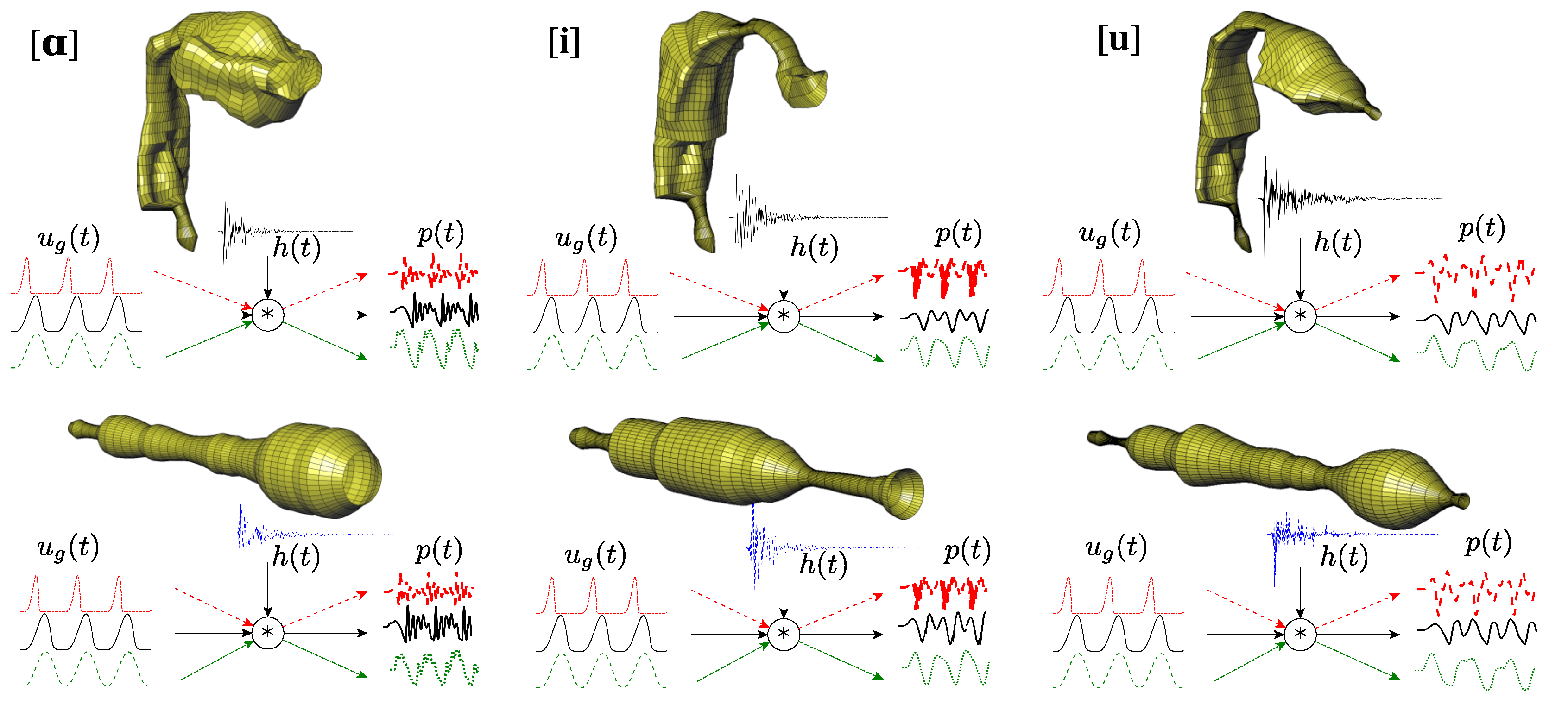
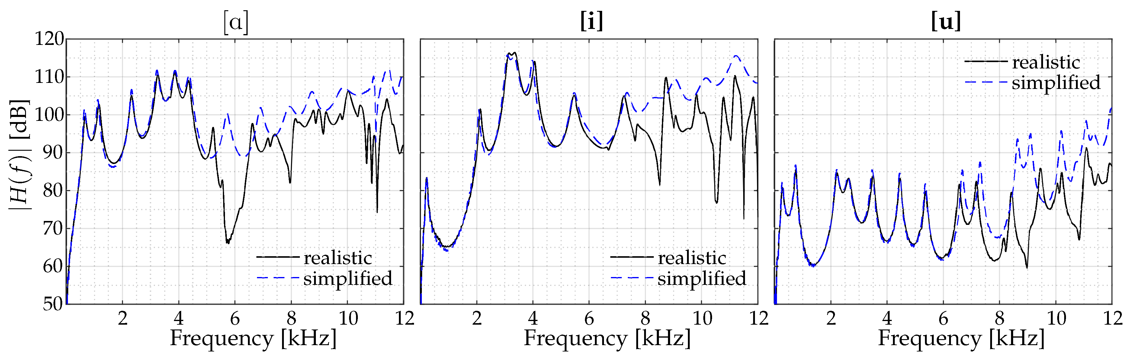
2.2. Vocal Tract Impulse Response

The impulse response of each vocal tract was obtained from the time-domain FEM simulations [11]. The propagation of acoustic waves within the 3D vocal tracts was provided by the FEM solution to the acoustic wave equation:

$$\begin{array}{c}\hfill {\partial }_{tt}^{2}p-c_0^2{\nabla }^{2}p=0,\end{array}$$

(1)

where $p(\mathit{x},t)$ stands for the acoustic pressure, ${\partial }_{tt}^2$ for the second order time derivative, and $c_0$ for the speed of sound. $c_0$ was set to the usual value of 350 m/s. An exterior domain was included to let waves emanate from the mouth and account in this way for radiation losses. A perfectly matched layer (PML) was imposed on the computational domain boundaries to prevent wave reflections. Wall losses were considered by prescribing a boundary admittance coefficient $\mu$ on the vocal tract walls which was set to $\mu =0.005$. Sound waves were generated within the vocal tract imposing a volume velocity $u_g\left(t\right)$ on the glottal cross-sectional area. Specifically, the following Gaussian pulse was used:

$$u_g\left(t\right)=e^{-{\left[(t-T_{gp})/0.29T_{gp}\right]}^2}[{\mathrm{m}}^3/\mathrm{s}],$$

(2)

with $T_{gp}=0.646/f_c$ and $f_c=10$ kHz.

Numerical simulations were performed with a sampling frequency of $f_s=8000$ kHz. This unusually large value was selected to ensure the stability of the explicit discrete time scheme used to solve the wave Equation (1). Time events of 20 ms were simulated, tracking the acoustic pressure, $p_0\left(t\right)$ at a mesh node located 4 cm away from the mouth exit. The vocal tract transfer function $H\left(f\right)$ was then obtained as:

$$H\left(f\right)=\frac{P_o\left(f\right)}{U_g\left(f\right)},$$

(3)

with $P_o\left(f\right)$ and $U_g\left(f\right)$ respectively being the Fourier transforms of $p_o\left(t\right)$ and $u_g\left(t\right)$. Note that this compensates for the slight spectral decay introduced by the Gaussian pulse. $H\left(f\right)$ was computed up to 12 kHz in order to generate speech at 24 kHz. This sampling frequency allowed us to cover the whole 8 kHz octave band, in which the HFE levels would be computed.

Figure 2 shows the computed vocal tract transfer functions $H\left(f\right)$ of $[ɑ]$, [i], and [u] for the realistic and simplified geometries. Observe that below 5 kHz the two representations behaved very similarly, whereas above that frequency strong differences emerged. This is consistent with the results presented in [5], where it was observed that plane wave propagation, which dominates below 5 kHz, is barely affected by the cross-sectional shape and vocal tract bending. Beyond that limit, however, higher order modes also propagate and play a significant role in the realistic configurations. In contrast, radial symmetry prevents the onset of most higher order modes in the simplified vocal tracts for the examined frequency range [4,5]. As observed in Figure 2, the depicted vocal tract transfer functions show an almost flat global trend in contrast to the spectral characteristics of speech because they do not include the effect of the glottal source.

The vocal tract impulse responses $h\left(t\right)$ were finally obtained from the inverse Fourier transform of the vocal tract transfer functions $H\left(f\right)$ (see Figure 1).

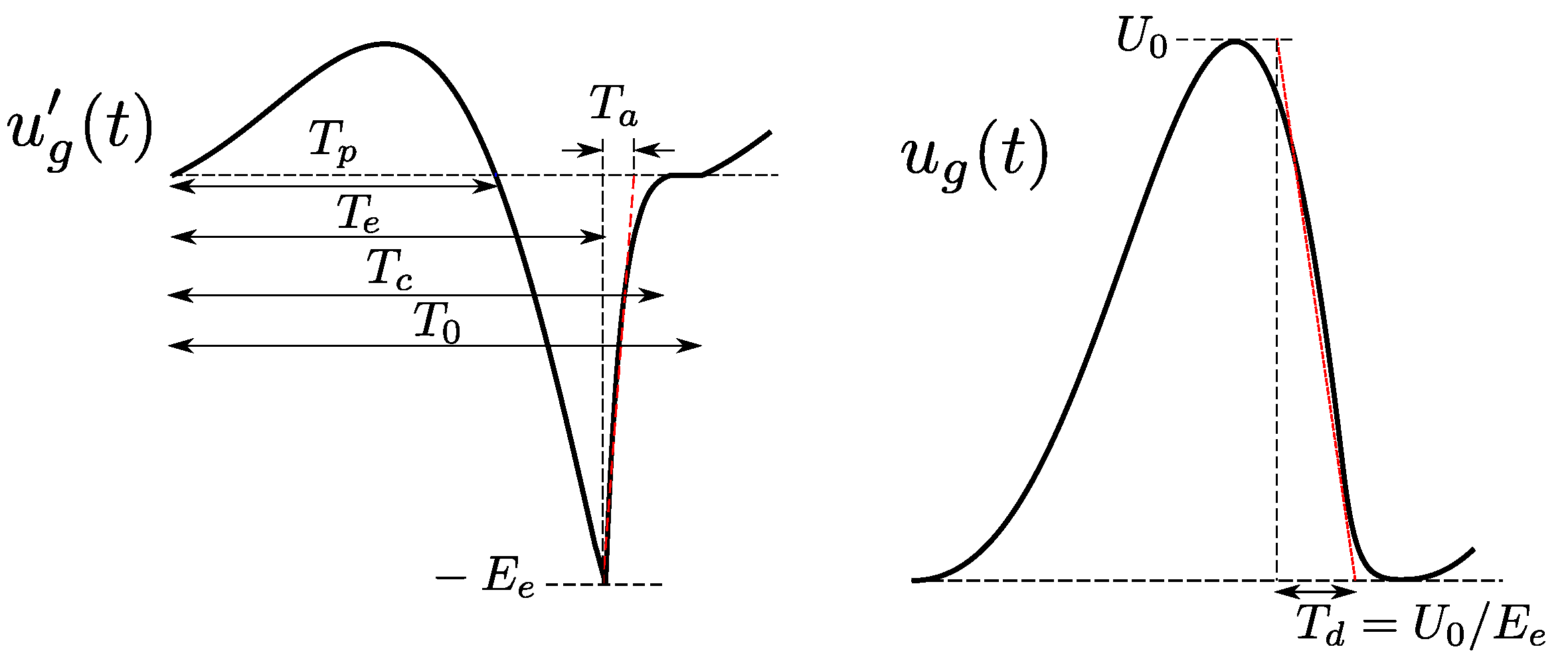
2.3. Voice Source Signal

Voice source signals were generated according to the LF model [12]. Specifically, Kawahara’s implementation [22] was chosen to obtain aliasing-free glottal flow derivative waveforms $u_g^{\prime }\left(t\right)$. The shape of a glottal pulse is controlled by the parameters $T_p$, $T_e$, $T_a$, $T_c$, and $T_0$ (see Figure 3). However, this control can be simplified as described in the transformed LF model [16]. The latter reduces parameter redundancy in the glottal pulse description. To this end, a global waveshape parameter, $R_d$, is introduced as:

$$R_d=\frac{T_d}{T_0}\frac{1}{110}=\frac{U_0}{E_e}\frac{F0}{110},$$

(4)

where $T_d$ is the declination time, $T_0$ the period, and $F0$ the fundamental frequency. The declination time $T_d$ corresponds to the quotient between the glottal flow peak $U_0$ and the negative amplitude of the differentiated glottal flow $E_e$. The scale factor was chosen so as to make the numerical value of $R_d$ the same as the declination time in seconds for $F0=110$ Hz [16]. The glottal shape parameter $R_d$ was integrated into Kawahara’s implementation, thereby allowing us to simulate from a tense, very adducted phonation ($R_d=0.3$) to a lax, very abducted phonation ($R_d=2.7$). $T_p$, $T_e$, and $T_a$ are derived from $R_d$ according to the equations in [16] and $T_c$ is set to $T_0$. The glottal flow $u_g\left(t\right)$ is computed by performing the cumulative integration of $u_g^{\prime }\left(t\right)$ using the composite trapezoidal rule [23].

Furthermore, the voice source model was extended to incorporate aspiration noise, $S_{AH}\left(t\right)$, which is added to the glottal flow $u_g\left(t\right)$. To this end, the method presented in [24] was implemented. This consists of automatically generating the temporal dynamics of $S_{AH}\left(t\right)$ according to the voice source parameters as follows:

$$S_{AH}\left(t\right)=AH{E}_e^{1.35}F{0}^{1.05}n\left(t\right)\sqrt{\frac{U_{ac}}{U_0}{u}_g\left(t\right)+U_{dc}},$$

(5)

where $U_{ac}=(379/R_d)-91$, $U_{dc}=83T_d+34$ and $T_d=110T_0{R}_d$, according to [24]. The noise amplitude factor $AH$ was perceptually adjusted to $3\times {10}^{-14}$. The noise signal $n\left(t\right)$ was generated by filtering white Gaussian noise with a 2nd order Butterworth bandpass filter with cutoff frequencies of 300 and 3000 Hz as in [1]. Finally, a SoX resampling (http://sox.sourceforge.net/SoX/Resampling) was incorporated to adapt the glottal flow signals originally generated at 44,100 Hz to the sampling rate at which the speech signals were synthesised (24 kHz).

The glottal flow signals generated for this work cover the $R_d$ range $[0.3,2.7]$ [16], considering 49 logarithmically spaced values of $R_d$ (24 steps from 0.3 to 1 and 24 more steps from 1 to 2.7). Regarding $F0$, a pitch contour was extracted from a real sustained vowel lasting for 2 s. This curve was successively pitch-shifted from a $F0$ mean value of 75.6 Hz to 240 Hz in 81 steps of 0.25 semitones, thereby covering the male speech range [25]. For each possible combination of $R_d$ and $F0$ values, two glottal flow versions were obtained with and without aspiration noise. The pulse amplitude, $U_0$, was selected to have $70{\mathrm{dB}}_{\mathrm{SPL}}$ with the realistic geometry, $F0=120$ Hz and $R_d=1$, which resulted in values $U_0=6.296\times {10}^{-5}{\mathrm{m}}^3/\mathrm{s}$ for vowel $[ɑ]$, $U_0=3.455\times {10}^{-5}{\mathrm{m}}^3/\mathrm{s}$ for [i] and $U_0=6.657\times {10}^{-5}{\mathrm{m}}^3/\mathrm{s}$ for [u].

2.4. Acoustic Analysis

The Welch’s power spectral density (PSD) estimate of each synthesised vowel was computed using a 2048-point FFT, with a 15 ms Hanning window and 50% overlap. The PSD was scaled by the equivalent noise bandwidth of the window to get the long-term average spectrum (LTAS). Moreover, HFE levels were computed as the integral of the PSD estimate within the 8 kHz octave band, as in [10,26] and in the three 1/3 octaves conforming that band, i.e., 6.3 kHz, 8 kHz, and 10 kHz. In the same way, the overall energy levels were obtained by considering the full bandwidth from 0 Hz to 12 kHz. The 16 kHz octave band was not considered in this study because its HFE variations have been shown to be almost perceptually irrelevant, see [10].

3. Results

The vowels [$ɑ$], [i], and [u] were synthesised modifying the glottal source model in the whole phonation range, defined in this work as the space comprising fundamental frequencies $F0\in [75.6,240]$ Hz for $R_d\in [0.3,2.7]$. Amplitude variations of the glottal pulses, $U_0$, could have also been incorporated in the study. However, they were not considered because they simply produce a level increment proportional to $U_0$. For instance, doubling the amplitude of $U_0$ simply generates a constant level offset of $+6\mathrm{dB}$ at all frequencies.

In the following subsections we will start examining tense, modal, and lax phonations with $R_d=\{0.3,1,2.7\}$, respectively, for an intermediate $F0$ value of 120 Hz. The analysis will be then extended over the whole simulated phonation range, namely for $(F0,R_d)\in [75.6,240]\times [0.3,2.7]$.

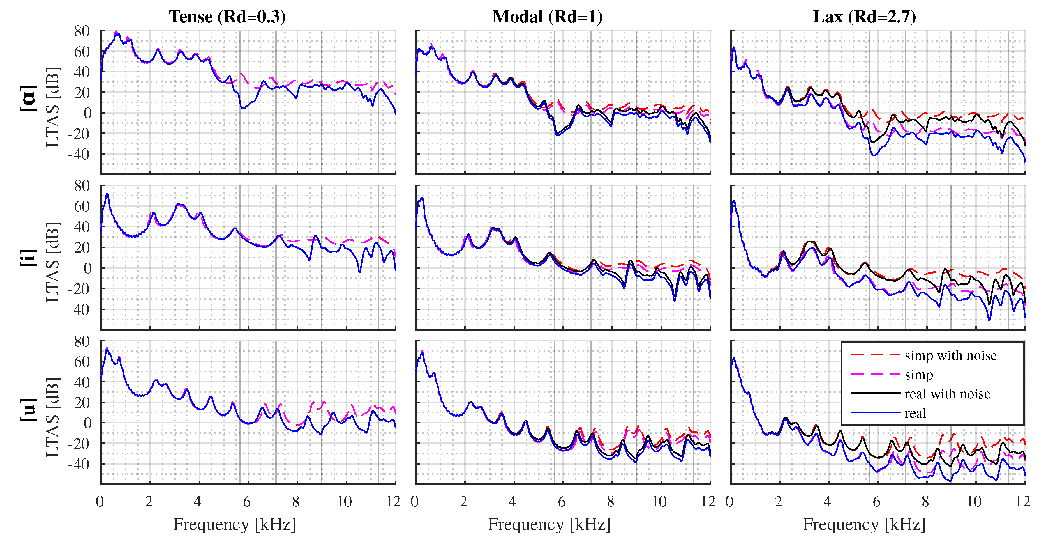
3.1. Analysis of Tense, Modal, and Lax Phonations for Fixed $F0$ and $R_d$ Values

Figure 4 shows the LTAS of vowels [$ɑ$], [i], and [u] for tense, modal, and lax phonations ($R_d=\{0.3,1,2.7\}$) with $F0=120$ Hz. The figure thus contains nine subplots covering all possible combinations. In turn, each subplot presents four curves. Those correspond to the results with the realistic and simplified vocal tract geometries for activated and deactivated aspiration noise. The overall and HFE levels of the LTAS curves are shown in

Table 1. Overall and high frequency energy (HFE) levels (in dB) obtained in the realistic and simplified vocal tract configurations of vowels $[ɑ]$, [i], and [u]. Values correspond to vowels with a tense ($R_d=0.3$), a modal ($R_d=1$), and a lax ($R_d=2.7$) phonation without considering aspiration noise. The values in parentheses denote the increment in dB obtained due to adding aspiration noise.

Vowel	Geometry	${\mathit{R}}_{\mathit{d}}$	Overall	1/1 Octave Band	1/3 Octave Band
				8 kHz	6.3 kHz	8 kHz	10 kHz
$[ɑ]$	realistic	0.3	82.3 (+0.0)	41.5 (+0.2)	35.3 (+0.1)	37.6 (+0.2)	37.2 (+0.2)
		1.0	70.0 (+0.0)	14.5 (+3.8)	8.7 (+3.0)	10.6 (+3.7)	9.8 (+4.4)
		2.7	63.5 (+0.0)	−4.5 (+14.4)	−10.3 (+13.1)	−8.5 (+14.3)	−9.1 (+15.2)
	simplified	0.3	83.5 (+0.0)	47.4 (+0.1)	43.4 (+0.1)	42.4 (+0.2)	41.9 (+0.2)
		1.0	71.4 (+0.0)	20.5 (+3.5)	17.0 (+2.8)	15.3 (+3.6)	14.5 (+4.4)
		2.7	64.9 (+0.0)	1.6 (+13.8)	−1.8 (+12.4)	−3.7 (+14.3)	−4.4 (+15.3)
$\left[\mathrm{i}\right]$	realistic	0.3	73.6 (+0.0)	41.0 (+0.2)	37.0 (+0.1)	37.9 (+0.2)	31.8 (+0.2)
		1.0	70.0 (+0.0)	14.2 (+3.3)	10.6 (+2.7)	10.9 (+3.5)	4.4 (+4.4)
		2.7	65.6 (+0.0)	−4.7 (+13.4)	−8.2 (+12.3)	−8.0 (+13.8)	−14.5 (+15.2)
	simplified	0.3	73.4 (+0.0)	44.8 (+0.2)	38.5 (+0.1)	40.7 (+0.2)	40.5 (+0.2)
		1.0	70.0 (+0.0)	17.8 (+3.7)	12.2 (+2.7)	13.7 (+3.6)	13.1 (+4.4)
		2.7	65.6 (+0.0)	−1.0 (+14.0)	−6.6 (+12.2)	−5.0 (+13.8)	−5.7 (+15.2)
$\left[\mathrm{u}\right]$	realistic	0.3	74.0 (+0.0)	22.8 (+0.2)	19.6 (+0.1)	16.3 (+0.2)	18.0 (+0.3)
		1.0	70.0 (+0.0)	−4.0 (+3.6)	−6.9 (+3.0)	−10.6 (+3.3)	−9.4 (+4.5)
		2.7	64.2 (+0.0)	−23.2 (+14.1)	−26.4 (+13.5)	−29.3 (+13.3)	−28.3 (+15.3)
	simplified	0.3	75.0 (+0.0)	29.9 (+0.2)	21.5 (+0.1)	25.4 (+0.2)	27.0 (+0.2)
		1.0	71.1 (+0.0)	2.7 (+4.0)	−5.2 (+3.2)	−1.7 (+3.7)	−0.4 (+4.4)
		2.7	64.2 (+0.0)	−16.0 (+14.4)	−23.6 (+12.6)	−20.5 (+14.2)	−19.2 (+15.1)

for the 8 kHz octave frequency band and also for its corresponding 1/3 octave bands, 6.3 kHz, 8 kHz, and 10 kHz. Values in parentheses indicate the level rise produced by including aspiration noise in the glottal source model.

Let us first focus on the comparison between the realistic and simplified vocal tract geometries. Looking at Figure 4, we can observe that the vocal tract geometry did not have a significant effect on frequencies below ∼5 kHz, as already mentioned before, in contrast to the high frequency range. As explained, this is because planar modes mainly propagate at lower frequencies, whereas the higher order ones mostly appear in the high frequency range. This was clearly the case for the realistic geometry. Note, for instance, that a large valley is produced close to 6 kHz in the realistic configuration of $[ɑ]$ (generated by a transverse mode, see [5]), whereas a resonance appears instead in the simplified configuration. The lack of higher order modes in the latter due to radial symmetry will allow us to determine their influence by comparing the results from the two configurations.

In general, higher order modes diminished the HFE levels, regardless of the phonation type and examined vowel. Note that in the 8 kHz octave band of Table 1 the level of the realistic geometry became between $5.6$ dB and $6.1$ dB lower than that of the simplified geometry for vowel $[ɑ]$, between $3.6$ and $4.3$ dB for vowel [i], and between $6.7$ and $7.5$ dB for [u]. More details can be obtained from the 1/3 octave bands levels at 6.3 kHz, 8 kHz, and 10 kHz. The first one at 6.3 kHz only presents small spectral differences for [u] and [i], which ranged from $1.8$ dB to $2.8$ dB for [u] and were of the order of $1.5\mathrm{dB}$ for [i]. Actually, this 1/3 octave band did not contain higher order modes for these vowels (see Figure 4). Conversely, the dip around 6 kHz in the realistic $[ɑ]$ vowel caused level decreases of between $7.8$ dB and $8.5$ dB. For this vowel, the onset of higher order modes took place at a lower frequency since vowel $[ɑ]$ has a bigger oral cavity than [u] and [i]. In the second 1/3 octave band, centred at 8 kHz, the largest differences were found for [u]. In this case, the realistic configuration presented a valley close to 9 kHz, whereas resonances appeared for the simplified geometry. This results in variations ranged from $8.8$ dB to $9.6$ dB. Finally, [i] and [u] exhibited the largest deviations for the third 1/3 octave band at 10 kHz, which varied from $8.8$ dB to $9.0$ dB for the realistic configuration. According to [10], minimum difference limen scores of about 1 dB were obtained for normal-hearing listeners in the 1/1 octave band of 8 kHz. Therefore, one could hypothesise taking into account the aforementioned differences, that higher order modes could be perceptually relevant. However, this relevance may also depend on the HFE levels, which in turn greatly depend on the glottal source.

The glottal source not only modified the overall energy level but also introduced a spectral decay that can be appreciated by comparing the LTAS in Figure 4 with the $H\left(f\right)$ of Figure 2. This decay, also known as the spectral tilt, is strongly dependent on the phonation type. In Figure 4, it can be observed that the laxer the phonation (i.e., for growing $R_d$) the stronger the spectral tilt, especially at higher frequencies. For instance, moving from the modal phonation to the lax one produces an overall energy decay between $4.4$ dB and $6.9$ dB, considering all values in Table 1. However, this reduction is much larger in the high frequency range. It can reach ∼19 dB if no aspiration noise is considered. When aspiration noise is present, the decrease was not so prominent and only ranged from $8.0$ dB to $9.4$ dB. On the other hand, going from a modal to a tense phonation resulted in the opposite behaviour. The spectral tilt was reduced, which increased the overall levels between $3.5$ dB and $12.2$ dB. Again, the HFE levels were more sensitive and increased from $23.1$ dB to $27.4$ dB. It is worthwhile observing that in this case the aspiration noise did not play a determinant role, since as the LTAS of Figure 4 shows, the tense phonation remained unaltered.

Let us then analyse the influence of aspiration noise in more detail. As seen from Table 1, the aspiration noise had no effect at all on the overall levels of any of the analysed configurations. It only affected the HFE content, resulting in significant energy increments for laxer phonations but in negligible differences for the tense ones. Level increments in the 8 kHz octave band of Table 1 were less than $0.2\mathrm{dB}$ for the latter. In the case of modal phonation, the energy slightly increased beyond 4 kHz (see Figure 4), which resulted in a level rise from $3.3$ dB to $4.0$ dB in the 8 kHz octave band. As expected, the most sensitive phonation type was the lax one, which was strongly influenced by aspiration starting from ∼2.5 kHz. The 8 kHz octave band levels increased from $13.4$ dB to $14.4$ dB in this case.

To summarise, higher order modes diminished HFE levels between $3.6$ dB and $7.5$ dB in the 8 kHz octave band when considering all tested configurations. These level reductions were comparable to those in [10] and could therefore be perceptually relevant. Nevertheless, the differences induced by the higher order modes would only be perceivable if the energy input at the high frequency range was substantial. This seems to be the case of the tense phonation, whose levels in the aforementioned frequency band were higher than $41\mathrm{dB}$ for $[ɑ]$ and [i], and above $22\mathrm{dB}$ for [u] (see Table 1). When the phonation was modal, higher order modes might still have been relevant for $[ɑ]$ and [i], which presented HFE levels above $14\mathrm{dB}$, in contrast with [u], where the levels remained between $-4.0$ dB and $6.7$ dB. Finally, in the case of a lax phonation, perceptually significant HFE values could only be achieved for $[ɑ]$ and [i] if aspiration noise was considered (with variations between $8.7$ dB and $15.4$ dB). Higher order modes became irrelevant for [u].

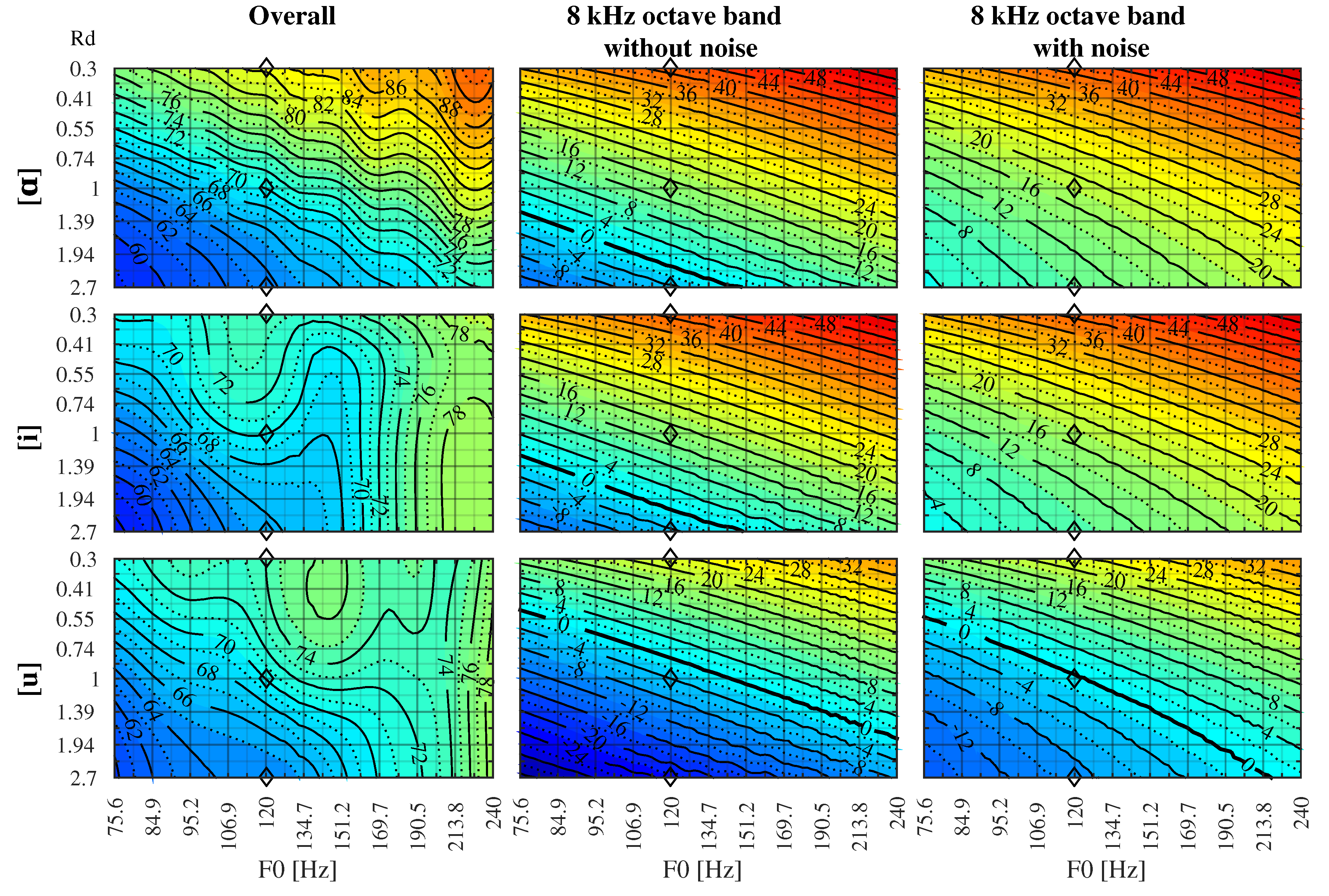
3.2. Analysis for the Whole Phonation Range

The analysis for the whole phonation range comprises of the overall and HFE levels in the 8 kHz octave band for the realistic geometry of the three vowels, with and without aspiration noise in the glottal source model. That results in the nine contour subplots are shown in Figure 5. A rainbow colour scale is used for all of them, with red and blue respectively representing the highest and lowest energy levels. Note that the realistic cases analysed in the previous Section 3.1 correspond to the vertical lines in the subplots, which have been indicated with a diamond symbol.

The colour maps in Figure 5 exhibit a pattern of diagonal contours with a general tendency to increase the overall and HFE levels from bottom left to top right. That is to say the minimum levels were obtained for the lowest $F0$ and laxest phonation, $R_d=2.7$, and gradually increased when moving to higher $F0$ and smaller $R_d$ values. This means that the obtained energy levels not only depended on $R_d$, as already observed in the previous Section 3.1, but also on the $F0$ of the excitation. In regards to the overall levels (first column in Figure 5), the lowest values were similar for all vowels ranging between $57.6$ dB and $59.7$ dB. In contrast, the highest levels depended on each vowel and reached $91.6\mathrm{dB}$, $80.4\mathrm{dB}$, and $78.8\mathrm{dB}$ for $[ɑ]$, [i], and [u], respectively. The vocal tract of vowel $[ɑ]$ produced the highest overall levels thanks to its first three formants, which are the most prominent ones as seen from the VTTFs in Figure 2. Moreover, these resonances took place below 2.5 kHz, where the energy decay of the tense voice source was still moderate (see the top-left subplot in Figure 4). On the other hand, the contours for the overall levels in Figure 4 present some deviations with respect to the aforementioned diagonal pattern, especially for [i] and [u]. These deviations occurred at those $F0$s that were sub-multiples of the frequency of each vowel first formant $F_1$. For instance, vowel $[ɑ]$ presented level increases at $F0=168.3$ Hz and $F0=224.3$ Hz, which correspond to $F_1/4$ and $F_1/3$, respectively. This effect was even more exaggerated for vowels [i] and [u], since they had a lower $F_1$ frequency. Note that the levels of these two vowels significantly increased at 110 Hz and 144.5 Hz, i.e., at $F_1/2$.

An even more interesting analysis is the examination of HFE content at 8 kHz with and without aspiration noise. When comparing the second and third columns in Figure 5, we can appreciate how the inclusion of aspiration curves the iso-contours in the bottom left corner of the subplots. Hence, the impact of aspiration noise increased as the phonation became laxer, whereas its effect was negligible for tense phonations ($R_d<0.74$) as quoted in Section 3.1. The contour maps also revealed the effect of aspiration noise increased for decreasing $F0$. When the aspiration noise was not considered, the HFE levels were similar for $[ɑ]$ and [i], ranging between $-14.6$ dB and $54.5$ dB, while they were much lower for vowel [u] with variations ranging from $-32$ dB to 33 dB. Vowel [u] produced lower HFE values despite having similar overall levels to [i]. On the other hand, when the aspiration noise was added, the minimum HFE levels for $[ɑ]$ and [i] were 3.3 and $2.1\mathrm{dB}$, respectively. Thus, the levels for these two vowels were above the theoretically audible threshold of $0\mathrm{dB}$, in the analysed phonation range. Conversely, the region of [u] with higher $R_d$ values and lower $F0$s remained below $0\mathrm{dB}$ even if aspiration noise was incorporated. The minimum HFE level for this vowel was $-15.7\mathrm{dB}$. Therefore, depending on the phonation type and also on the vowel, the HFE levels may have been too small to perceive differences in simulations with the realistic or simplified vocal tract geometries. This may occur for high $R_d$ values and/or low $F0$s, especially if there was no aspiration noise. In this respect, the presence of the latter seemed to suffice to obtain audible HFE levels for vowels $[ɑ]$ and [i], but not for [u], in the very lax region.

Let us next examine the influence of the geometry and consequently that of higher order modes in the considered phonation range. To do so, HFE level differences between the vowels generated with the realistic and simplified geometries were computed for each combination of $F0$-$R_d$-AspirationNoise.

Table 2. HFE level mean increments (in dB) obtained for the simplified geometries with respect to the realistic ones. The values have been computed for the 8 kHz octave band and its corresponding 1/3 octave bands. The values in parentheses denote the additional increment in dB due to aspiration noise.

Vowel	1/1 Octave Band	1/3 Octave Band
	8 kHz	6.3 kHz	8 kHz	10 kHz
$[ɑ]$	6.0 (−0.2)	8.2 (−0.2)	4.8 (+0.0)	4.7 (+0.0)
$\left[\mathrm{i}\right]$	3.6 (+0.3)	1.5 (+0.0)	2.8 (+0.1)	8.8 (+0.0)
$\left[\mathrm{u}\right]$	6.8 (+0.4)	1.8 (+0.0)	9.2 (+0.3)	9.0 (+0.0)

depicts the mean increments of the simplified configuration over the realistic ones in 1/1 and 1/3 octave frequency bands. It is worth mentioning that the standard deviation of these increments was less than $0.3\mathrm{dB}$ for all vowels and bands, since the LF model does not consider the interaction between the vocal tract and the vocal folds. The differences obtained in the 8 kHz 1/1 octave band were similar for $[ɑ]$ and [u], with mean increments of $6.0\mathrm{dB}$ and $6.8\mathrm{dB}$, respectively. Nevertheless, vowel $[ɑ]$ primarily concentrated the differences in the first 1/3 octave band, while changes for [u] mainly occurred in the other two bands. In turn, differences for [i] basically manifested in the 10 kHz band, the mean increment in the 8 kHz 1/1 octave band being only ∼$3.6\mathrm{dB}$. All these values could slightly vary when aspiration noise is included (see the increments in parentheses in Table 2). Note that the above observations were in line with the analysis derived in Section 3.1 for the selected three pairs of $(F0,R_d)$.

4. Conclusions

In this work, we analysed the relevance of higher order modes in the 3D finite element synthesis of vowels $[ɑ]$, [i], and [u], considering different glottal source excitations. It was shown that higher order modes induced a reduction of between $3.6$ dB and $7.2$ dB in the HFE levels of the 8 kHz octave band which, according to previous works in literature, may be perceptually relevant. However, the influence of higher order modes strongly depended on the phonation type and fundamental frequency $F0$. Influence was greater for phonations with high HFE levels, such as the tense ones (small $R_d$), and/or for high $F0$s. On the other hand, HFE levels dropped rapidly for lax phonations and/or low $F0$s. The presence of aspiration noise could partially alleviate such decreases for $[ɑ]$ and [i] vowels. Conversely, the levels obtained for [u] suggested that differences between realistic and simplified geometries may not be perceptually relevant for this vowel when the phonation was lax, even if aspiration noise is included. Future work will focus on the perceptual validation of the results presented herein. To this end, we will generate pseudowords containing vowels and consonants to have a broader assessable phonetic context, instead of only considering sustained vowels. However, the synthesis of such utterances is still being developed in FEM-based approaches for voice simulation.

Finally, we would like to point out that the outcomes for the realistic vocal tracts in this work correspond to those of a specific individual. Analysis for other speakers may result in some differences, yet we believe that the reported general tendencies will still be valid for them. In the future, though, it would be interesting to extend the investigation to further MRI-based geometries and using other glottal source models as well.

References

1. Story, B.H. Phrase-level speech simulation with an airway modulation model of speech production. Comput. Speech Lang. 2013, 27, 989–1010. [Google Scholar] [CrossRef] [Green Version]
2. Birkholz, P. Modeling Consonant-Vowel Coarticulation for Articulatory Speech Synthesis. PLoS ONE 2013, 8, e60603. [Google Scholar] [CrossRef]
3. Arnela, M.; Dabbaghchian, S.; Guasch, O.; Engwall, O. MRI-based vocal tract representations for the three-dimensional finite element synthesis of diphthongs. IEEE/ACM Trans. Audio Speech Lang. Process. 2019, 27, 2173–2182. [Google Scholar] [CrossRef]
4. Blandin, R.; Arnela, M.; Laboissière, R.; Pelorson, X.; Guasch, O.; Hirtum, A.V.; Laval, X. Effects of higher order propagation modes in vocal tract like geometries. J. Acoust. Soc. Am. 2015, 137, 832–838. [Google Scholar] [CrossRef]
5. Arnela, M.; Dabbaghchian, S.; Blandin, R.; Guasch, O.; Engwall, O.; Van Hirtum, A.; Pelorson, X. Influence of vocal tract geometry simplifications on the numerical simulation of vowel sounds. J. Acoust. Soc. Am. 2016, 140, 1707–1718. [Google Scholar] [CrossRef] [Green Version]
6. Monson, B.B.; Hunter, E.J.; Lotto, A.J.; Story, B.H. The perceptual significance of high-frequency energy in the human voice. Front. Psychol. 2014, 5, 587. [Google Scholar] [CrossRef] [Green Version]
7. Vampola, T.; Horáček, J.; Švec, J.G. FE Modeling of Human Vocal Tract Acoustics. Part I: Production of Czech vowels. Acta Acust. United Acust. 2008, 94, 433–447. [Google Scholar] [CrossRef]
8. Takemoto, H.; Mokhtari, P.; Kitamura, T. Acoustic analysis of the vocal tract during vowel production by finite-difference time-domain method. J. Acoust. Soc. Am. 2010, 128, 3724–3738. [Google Scholar] [CrossRef]
9. Arnela, M.; Blandin, R.; Dabbaghchian, S.; Guasch, O.; Alías, F.; Pelorson, X.; Van Hirtum, A.; Engwall, O. Influence of lips on the production of vowels based on finite element simulations and experiments. J. Acoust. Soc. Am. 2016, 139, 2852–2859. [Google Scholar] [CrossRef] [Green Version]
10. Monson, B.B.; Lotto, A.J.; Ternström, S. Detection of high-frequency energy changes in sustained vowels produced by singers. J. Acoust. Soc. Am. 2011, 129, 2263–2268. [Google Scholar] [CrossRef] [Green Version]
11. Arnela, M.; Guasch, O. Finite element computation of elliptical vocal tract impedances using the two-microphone transfer function method. J. Acoust. Soc. Am. 2013, 133, 4197–4209. [Google Scholar] [CrossRef]
12. Fant, G.; Liljencrants, J.; Lin, Q. A four-parameter model of glottal flow. Speech Transm. Lab. Q. Prog. Status Rep. 1985, 26, 1–13. [Google Scholar]
13. Murtola, T.; Alku, P.; Malinen, J.; Geneid, A. Parameterization of a computational physical model for glottal flow using inverse filtering and high-speed videoendoscopy. Speech Commun. 2018, 96, 67–80. [Google Scholar] [CrossRef] [Green Version]
14. Erath, B.D.; Zañartu, M.; Stewart, K.C.; Plesniak, M.W.; Sommer, D.E.; Peterson, S.D. A review of lumped-element models of voiced speech. Speech Commun. 2013, 55, 667–690. [Google Scholar] [CrossRef]
15. Murphy, A.; Yanushevskaya, I.; Chasaide, A.N.; Gobl, C. Rd as a Control Parameter to Explore Affective Correlates of the Tense-Lax Continuum. In Proceedings of the Interspeech 2017, Stockholm, Sweden, 20–24 August 2017; pp. 3916–3920. [Google Scholar] [CrossRef]
16. Fant, G. The LF-model revisited. Transformations and frequency domain analysis. Speech Transm. Lab. Q. Prog. Status Rep. 1995, 36, 119–156. [Google Scholar]
17. Freixes, M.; Arnela, M.; Socoró, J.C.; Alías, F.; Guasch, O. Influence of tense, modal and lax phonation on the three-dimensional finite element synthesis of vowel [A]. In Proceedings of the IberSPEECH 2018, Barcelona, Spain, 21–23 November 2018; pp. 132–136. [Google Scholar] [CrossRef]
18. Aalto, D.; Aaltonen, O.; Happonen, R.P.; Jääsaari, P.; Kivelä, A.; Kuortti, J.; Luukinen, J.M.; Malinen, J.; Murtola, T.; Parkkola, R.; et al. Large scale data acquisition of simultaneous MRI and speech. Appl. Acoust. 2014, 83, 64–75. [Google Scholar] [CrossRef]
19. Arnela, M.; Guasch, O.; Alías, F. Effects of head geometry simplifications on acoustic radiation of vowel sounds based on time-domain finite-element simulations. J. Acoust. Soc. Am. 2013, 134, 2946–2954. [Google Scholar] [CrossRef]
20. Takemoto, H.; Adachi, S.; Mokhtari, P.; Kitamura, T. Acoustic interaction between the right and left piriform fossae in generating spectral dips. J. Acoust. Soc. Am. 2013, 134, 2955–2964. [Google Scholar] [CrossRef]
21. Story, B.H.; Titze, I.R.; Hoffman, E.A. Vocal tract area functions from magnetic resonance imaging. J. Acoust. Soc. Am. 1996, 100, 537–554. [Google Scholar] [CrossRef]
22. Kawahara, H.; Sakakibara, K.I.; Banno, H.; Morise, M.; Toda, T.; Irino, T. A new cosine series antialiasing function and its application to aliasing-free glottal source models for speech and singing synthesis. In Proceedings of the Interspeech 2017, Stockholm, Sweden, 20–24 August 2017; pp. 1358–1362. [Google Scholar] [CrossRef]
23. Davis, P.J.; Rabinowitz, P. Methods of Numerical Integration; Courier Corporation: North Chelmsford, MA, USA, 2007. [Google Scholar]
24. Gobl, C. Modelling aspiration noise during phonation using the LF voice source model. In Proceedings of the Interspeech 2006, Pittsburgh, PA, USA, 17–21 September 2006; pp. 965–968. [Google Scholar]
25. Pabon, P.; Ternström, S. Feature Maps of the Acoustic Spectrum of the Voice. J. Voice 2018, in press. [Google Scholar] [CrossRef]
26. Monson, B.B.; Lotto, A.J.; Story, B.H. Analysis of high-frequency energy in long-term average spectra of singing, speech, and voiceless fricatives. J. Acoust. Soc. Am. 2012, 132, 1754–1764. [Google Scholar] [CrossRef] [Green Version]
Figure 1. Synthesis of vowels [ ɑ ] , [i], and [u] with realistic vocal tract geometries (above) and their simplified counterparts of circular cross-sections set in a straightened midline (below). The output pressure signal p ( t ) is computed as the convolution of the glottal source u g ( t ) with the vocal tract impulse response h ( t ) obtained from a 3D FEM (finite element method) simulation. Three phonation type examples are represented in the figure: Tense (dashed red line), modal (solid black line), and lax (dotted green line).
Applsci 09 04535 g001
Figure 2. Vocal tract transfer function magnitude | H ( f ) | of vowels [ ɑ ] , [i], and [u] for realistic and simplified vocal tract geometries.
Applsci 09 04535 g002
Figure 3. Glottal flow u g ( t ) and its time derivative u g ( t ) according to the LF (Liljencrants–Fant) model [12]. T p is the rise time, T e is the duration of the open phase, T a corresponds to the effective duration of the return phase, T c is the location of the complete closure, T d is the declination time, and T 0 is the period. U 0 is the peak of the glottal flow and E e corresponds to the negative amplitude of the differentiated glottal flow.
Applsci 09 04535 g003
Figure 4. Long-term average spectra (LTAS) of the FEM synthesised vowels [ ɑ ] , [i], and [u] using the realistic and simplified vocal tract geometries with and without aspiration noise. Vowels were generated with a tense ( R d = 0.3 ), a modal ( R d = 1 ), and a lax ( R d = 2.7 ) phonation with F 0 = 120 Hz. Vertical lines depict the boundaries of the 1/3 octave bands 6.3 kHz, 8 kHz, and 10 kHz.
Applsci 09 04535 g004
Figure 5. Contour plots showing the overall and HFE levels (dB) in the 8 kHz 1/1 octave band for the realistic vocal tract geometry of vowels [ ɑ ] , [i], and [u]. HFE levels are computed with and without introducing aspiration noise in the glottal source model. Each plot depicts the equal level contours for the whole phonation range, representing the F 0 in the abscissas and the R d value in the ordinates. Diamonds represent the points analysed in Section 3.1.
Applsci 09 04535 g005