Mutual Information Input Selector and Probabilistic Machine Learning Utilisation for Air Pollution Proxies

 , ,
, ,
Abstract

1. Introduction
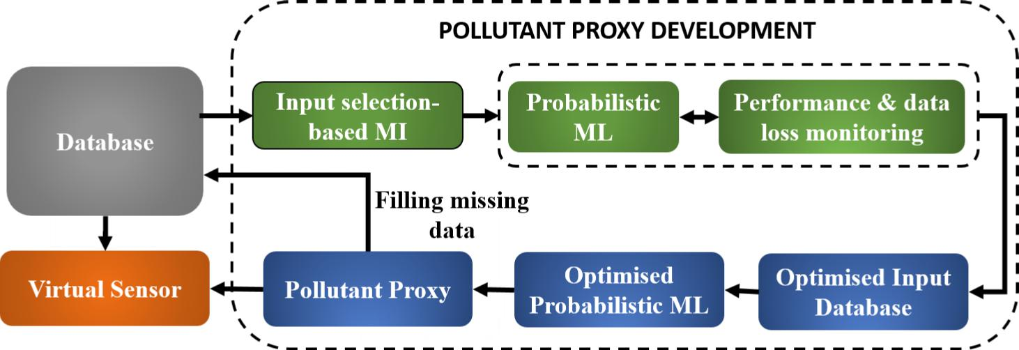
2. Methods
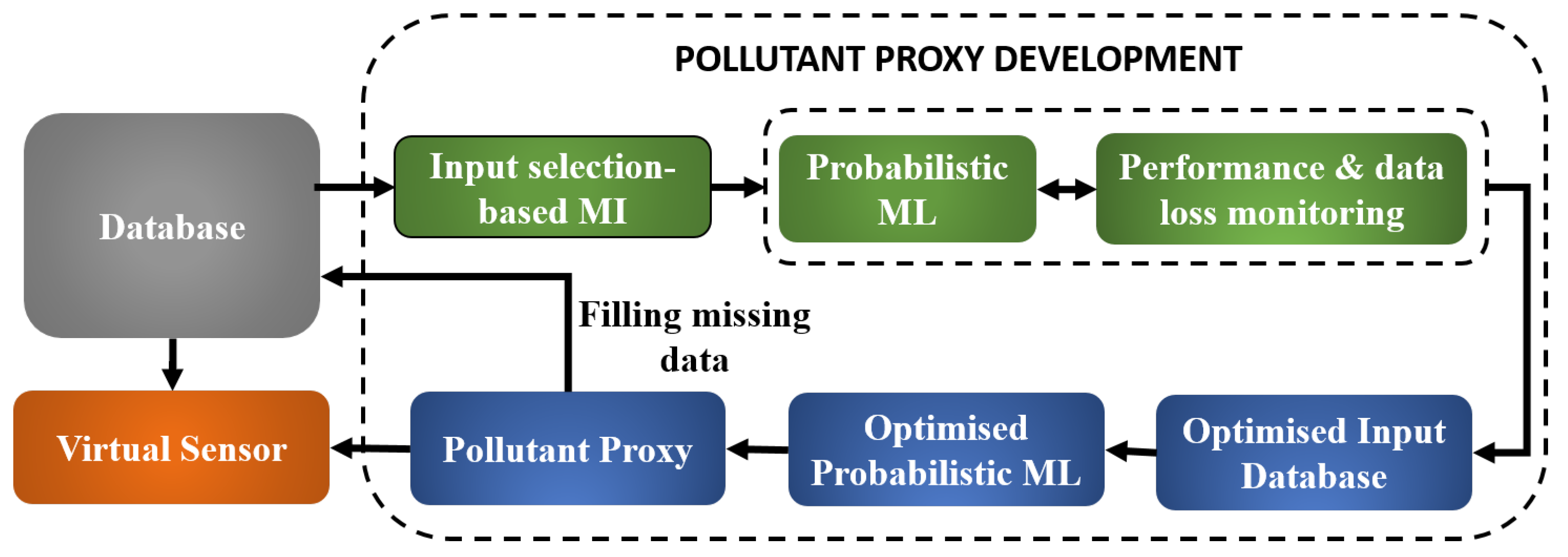
2.1. Input Selector: Mutual Information
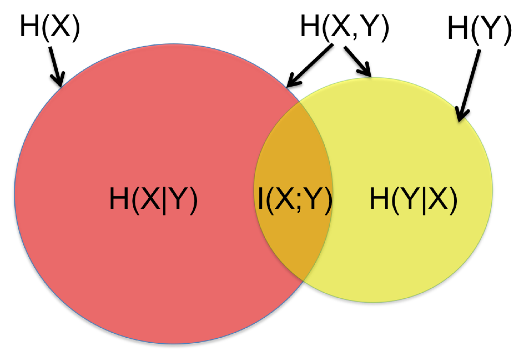
2.2. Probabilistic Machine Learning: Bayesian Neural Networks
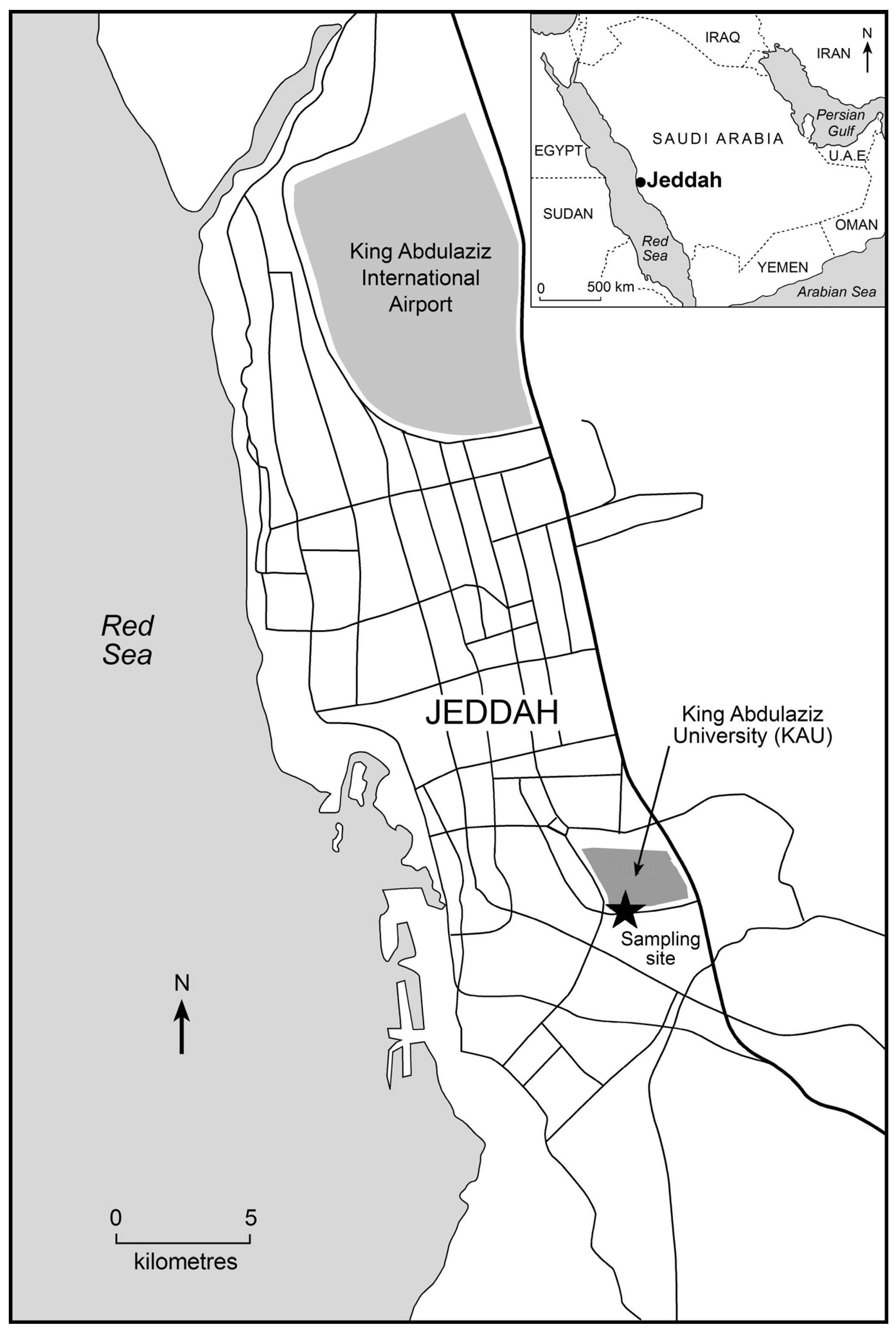
3. Case Study
4. Results and Discussion
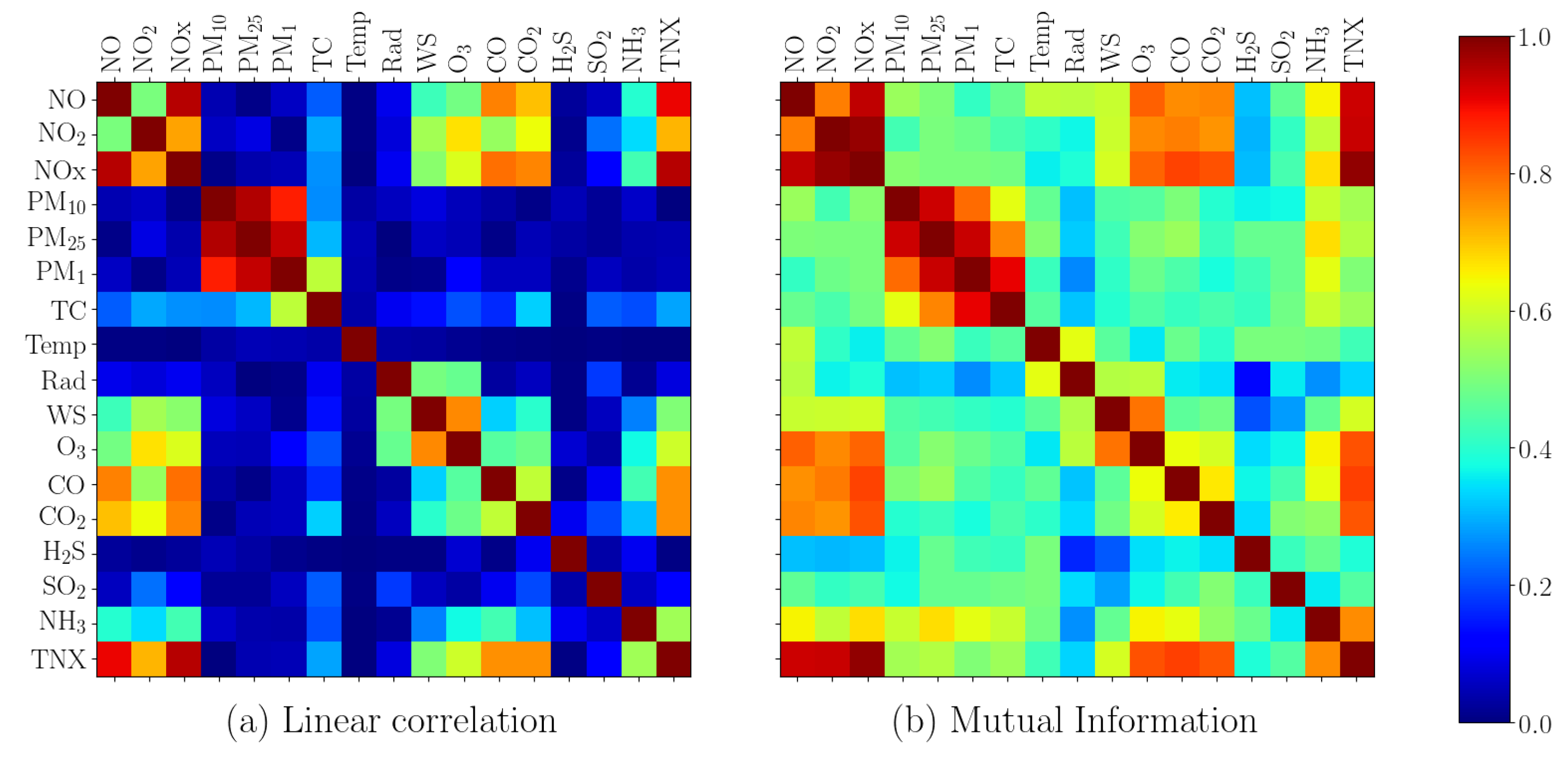
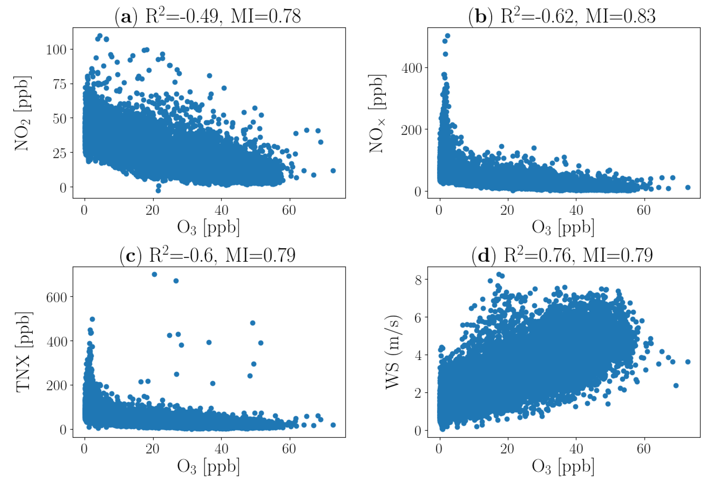
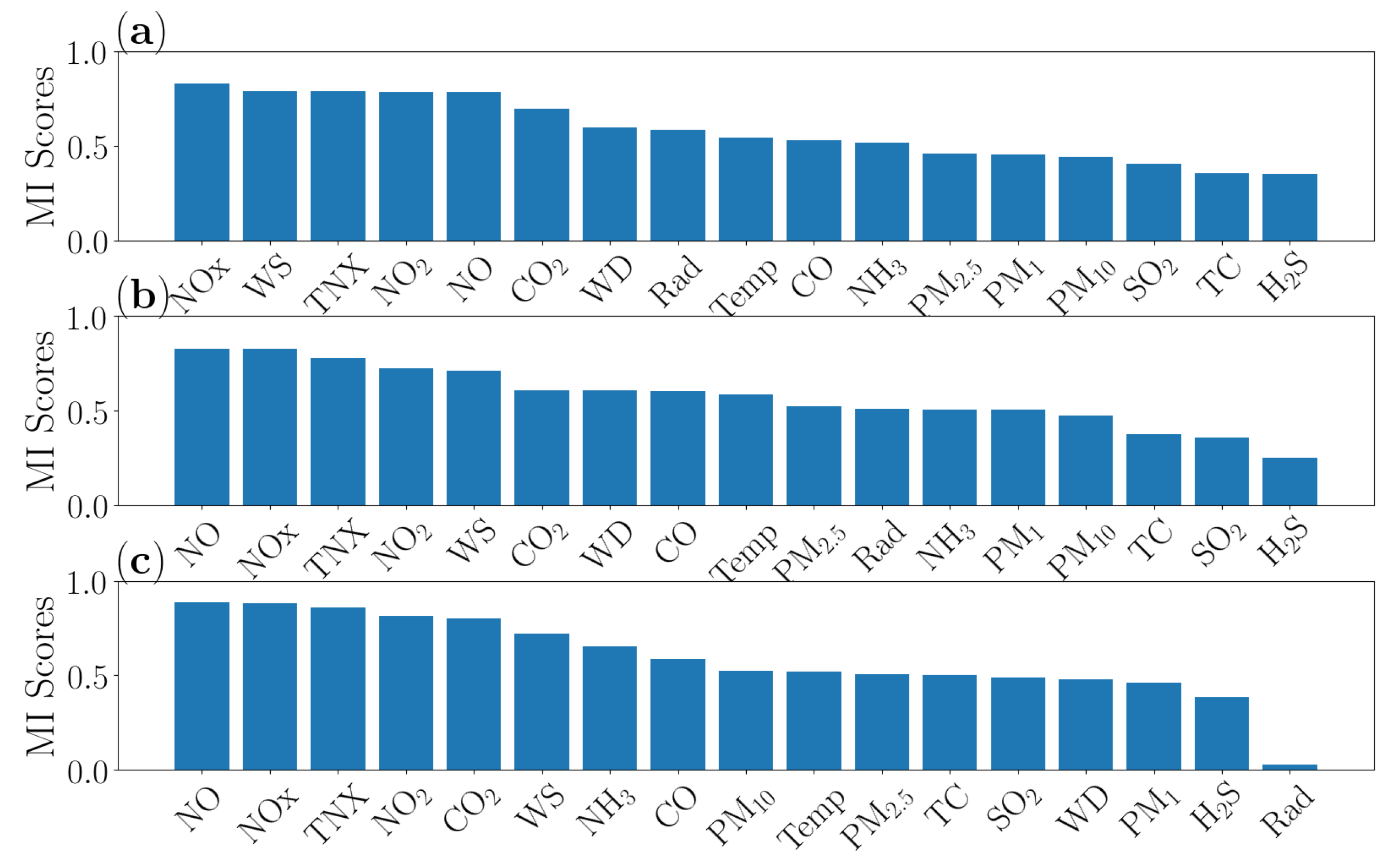
4.1. Data Analysis
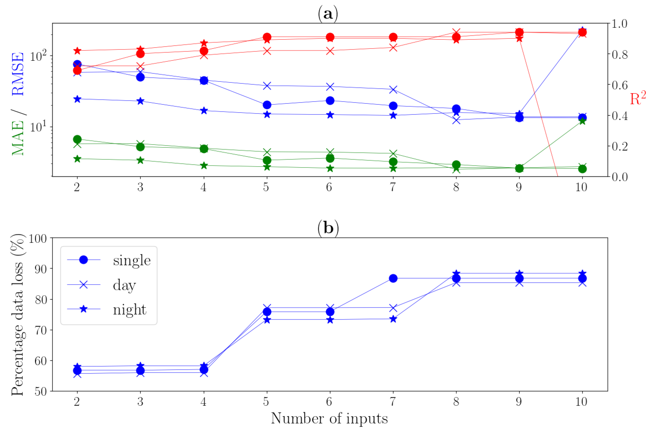
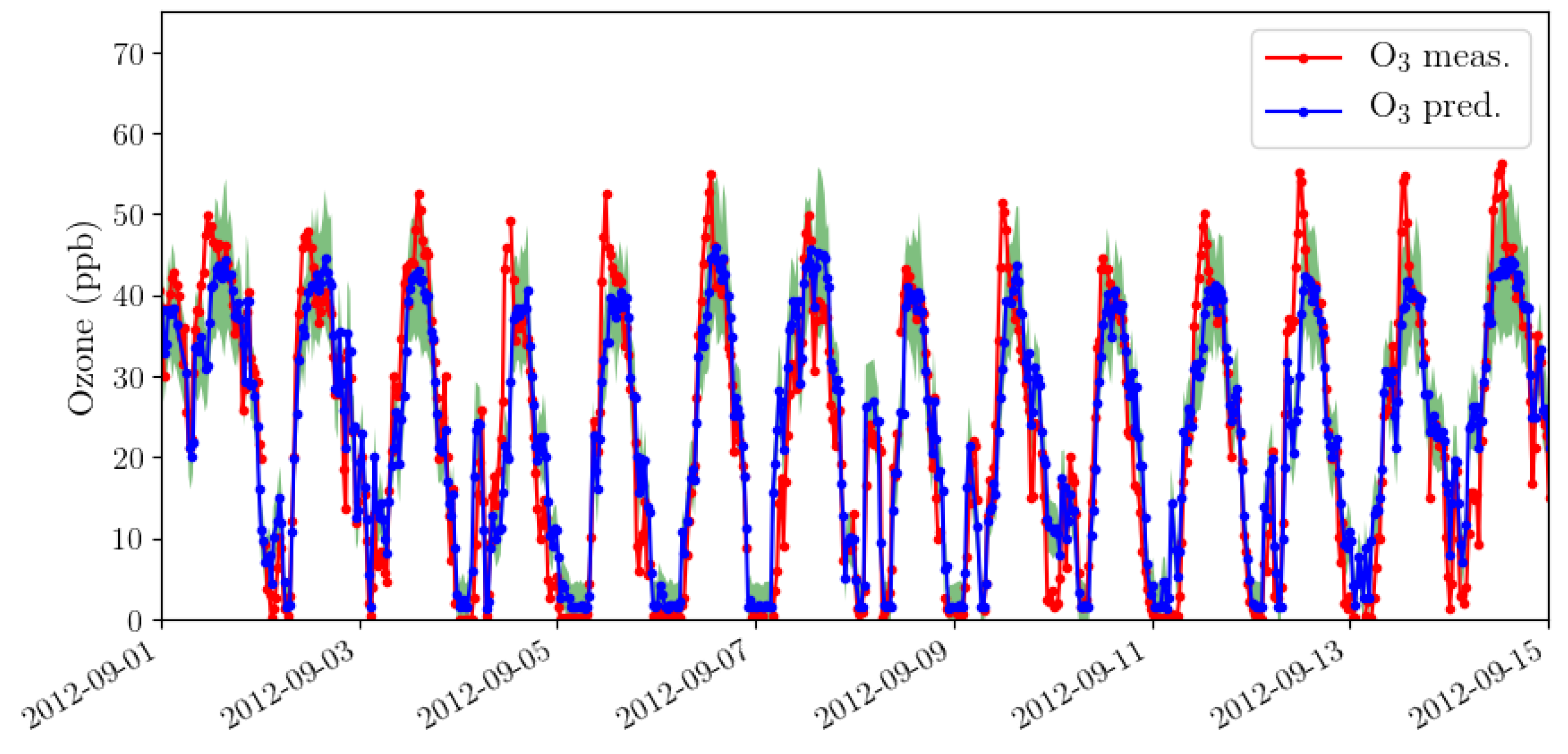
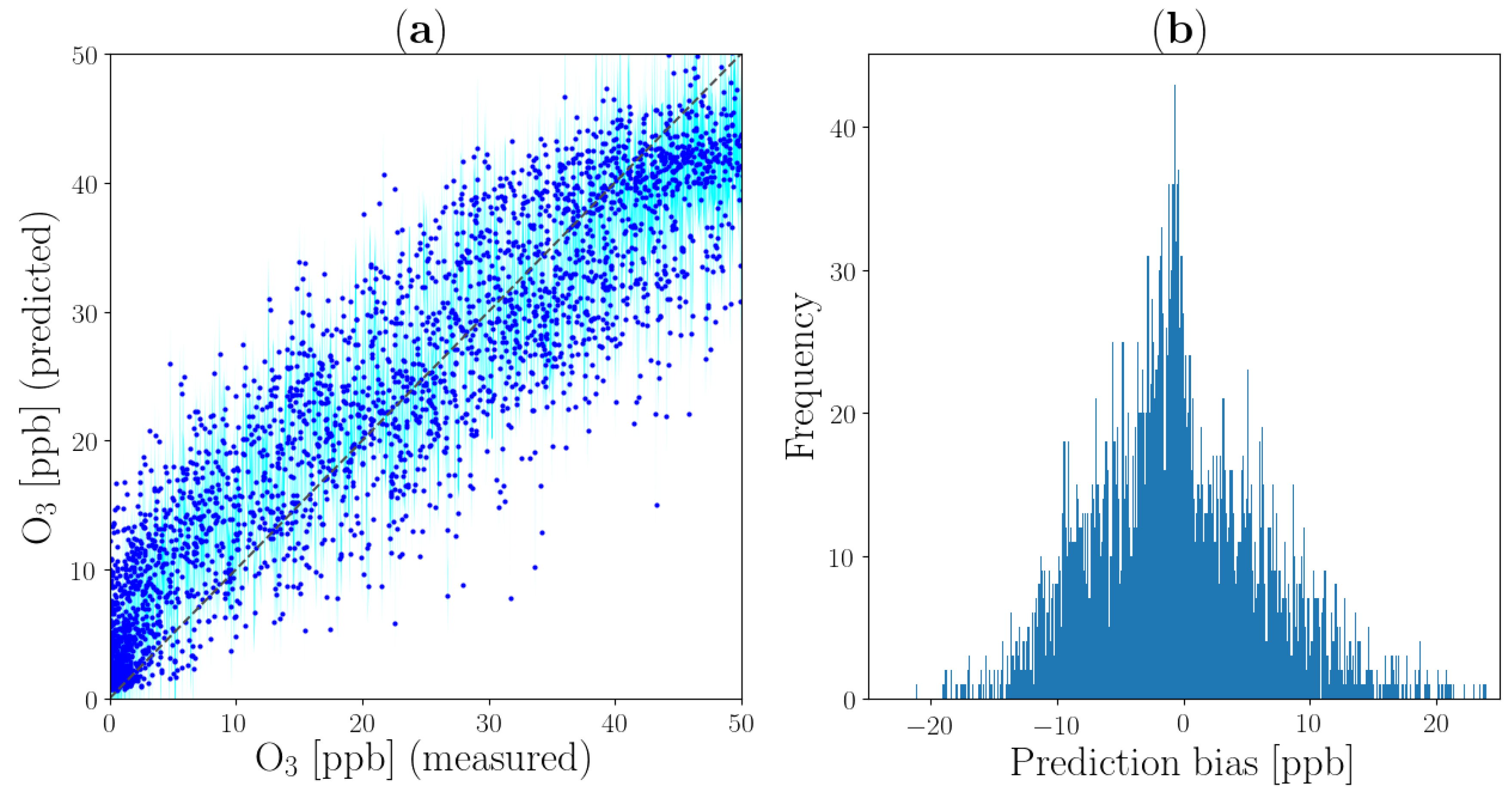
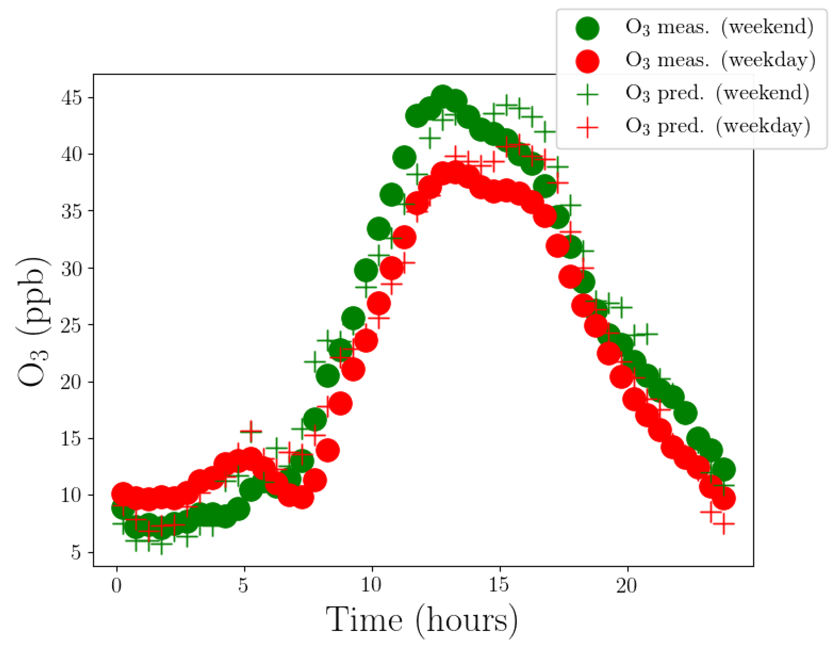
4.2. Performance Analysis
4.3. Discussion
5. Conclusions
Author Contributions
Funding
Acknowledgments
Conflicts of Interest
Abbreviations
| BNN | Bayesian Neural Network |
| MAE | Mean Absolute Error |
| ML | Machine Learning |
| MI | Mutual Information |
| NN | Neural Network |
| Nitric oxide | |
| Nitrogen dioxide | |
| Nitrogen oxides | |
| Ozone | |
| PCC | Pearson Correlation Coefficient |
| ppb | part per billion |
| RMSE | Root Mean Squared Error |
| SVM | Support Vector Machine |
| TNX | Xylene |
| WS | Wind Speed |
| WHO | World Health Organization |
References
- WHO Global Ambient Air Quality Database. Available online: https://www.who.int/airpollution/data/en/ (accessed on 17 August 2019).
- Wang, M.; Aaron, C.P.; Madrigano, J.; Hoffman, E.A.; Angelini, E.; Yang, J.; Laine, A.; Vetterli, T.M.; Kinney, P.L.; Sampson, P.D.; et al. Association between long-term exposure to ambient air pollution and change in quantitatively assessed emphysema and lung function. JAMA 2019, 322, 546–556. [Google Scholar] [CrossRef] [PubMed]
- Cairncross, E.K.; John, J.; Zunckel, M. A novel air pollution index based on the relative risk of daily mortality associated with short-term exposure to common air pollutants. Atmos. Environ. 2007, 41, 8442–8454. [Google Scholar] [CrossRef]
- Helmers, E.; Leitão, J.; Tietge, U.; Butler, T. CO2-equivalent emissions from European passenger vehicles in the years 1995–2015 based on real-world use: Assessing the climate benefit of the European “diesel boom”. Atmos. Environ. 2019, 198, 122–132. [Google Scholar] [CrossRef]
- Rockström, J.; Schellnhuber, H.J.; Hoskins, B.; Ramanathan, V.; Schlosser, P.; Brasseur, G.P.; Gaffney, O.; Nobre, C.; Meinshausen, M.; Rogelj, J.; et al. The world’s biggest gamble. Earth’s Future 2016, 4, 465–470. [Google Scholar] [CrossRef]
- Mølgaard, B.; Birmili, W.; Clifford, S.; Massling, A.; Eleftheriadis, K.; Norman, M.; Vratolis, S.; Wehner, B.; Corander, J.; Hämeri, K.; et al. Evaluation of a statistical forecast model for size-fractionated urban particle number concentrations using data from five European cities. J. Aerosol Sci. 2013, 66, 96–110. [Google Scholar] [CrossRef]
- Kumar, P.; Morawska, L.; Martani, C.; Biskos, G.; Neophytou, M.; Di Sabatino, S.; Bell, M.; Norford, L.; Britter, R. The rise of low-cost sensing for managing air pollution in cities. Environ. Int. 2015, 75, 199–205. [Google Scholar] [CrossRef]
- Chong, C.Y.; Kumar, S.P. Sensor networks: Evolution, opportunities, and challenges. Proc. IEEE 2003, 91, 1247–1256. [Google Scholar] [CrossRef]
- Junninen, H.; Niska, H.; Tuppurainen, K.; Ruuskanen, J.; Kolehmainen, M. Methods for imputation of missing values in air quality data sets. Atmos. Environ. 2004, 38, 2895–2907. [Google Scholar] [CrossRef]
- Rohde, R.A.; Muller, R.A. Air pollution in China: Mapping of concentrations and sources. PLoS ONE 2015, 10, e0135749. [Google Scholar] [CrossRef]
- Junger, W.; De Leon, A.P. Imputation of missing data in time series for air pollutants. Atmos. Environ. 2015, 102, 96–104. [Google Scholar] [CrossRef]
- Strigaro, D.; Cannata, M.; Antonovic, M. Boosting a weather monitoring system in low Income economies using open and non-conventional systems: data quality analysis. Sensors 2019, 19, 1185. [Google Scholar] [CrossRef] [PubMed]
- Carnevale, C.; Finzi, G.; Pisoni, E.; Volta, M.; Guariso, G.; Gianfreda, R.; Maffeis, G.; Thunis, P.; White, L.; Triacchini, G. An integrated assessment tool to define effective air quality policies at regional scale. Environ. Model. Softw. 2012, 38, 306–315. [Google Scholar] [CrossRef]
- Gupta, P.; Christopher, S.A.; Wang, J.; Gehrig, R.; Lee, Y.; Kumar, N. Satellite remote sensing of particulate matter and air quality assessment over global cities. Atmos. Environ. 2006, 40, 5880–5892. [Google Scholar] [CrossRef]
- Sofiev, M.; Galperin, M.; Genikhovich, E. A construction and evaluation of Eulerian dynamic core for the air quality and emergency modelling system SILAM. In Air Pollution Modeling and Its Application XIX; Springer: New York, NY, USA, 2008; pp. 699–701. [Google Scholar]
- Clifford, S.; Choy, S.L.; Hussein, T.; Mengersen, K.; Morawska, L. Using the generalised additive model to model the particle number count of ultrafine particles. Atmos. Environ. 2011, 45, 5934–5945. [Google Scholar] [CrossRef]
- Mølgaard, B.; Hussein, T.; Corander, J.; Hämeri, K. Forecasting size-fractionated particle number concentrations in the urban atmosphere. Atmos. Environ. 2012, 46, 155–163. [Google Scholar] [CrossRef]
- Von Bismarck-Osten, C.; Birmili, W.; Ketzel, M.; Weber, S. Statistical modelling of aerosol particle number size distributions in urban and rural environments—A multi-site study. Urban Clim. 2015, 11, 51–66. [Google Scholar] [CrossRef]
- Khalil, M.; Butenhoff, C.L.; Harrison, R. Ozone balances in urban Saudi Arabia. NPJ Clim. Atmos. Sci. 2018, 1, 27. [Google Scholar] [CrossRef]
- Alghamdi, M.A.; Al-Hunaiti, A.; Arar, S.; Khoder, M.; Abdelmaksoud, A.S.; Al-Jeelani, H.; Lihavainen, H.; Hyvärinen, A.; Shabbaj, I.I.; Almehmadi, F.M.; et al. A predictive model for steady state ozone concentration at an urban-coastal site. Int. J. Environ. Res. Public Health 2019, 16, 258. [Google Scholar] [CrossRef]
- Taylan, O. Modelling and analysis of ozone concentration by artificial intelligent techniques for estimating air quality. Atmos. Environ. 2017, 150, 356–365. [Google Scholar] [CrossRef]
- Gao, M.; Yin, L.; Ning, J. Artificial neural network model for ozone concentration estimation and Monte Carlo analysis. Atmos. Environ. 2018, 184, 129–139. [Google Scholar] [CrossRef]
- Arroyo, Á.; Herrero, Á.; Tricio, V.; Corchado, E.; Woźniak, M. Neural models for imputation of missing ozone data in air-quality datasets. Complexity 2018, 2018, 7238015. [Google Scholar] [CrossRef]
- Ortiz-García, E.; Salcedo-Sanz, S.; Pérez-Bellido, Á.; Portilla-Figueras, J.; Prieto, L. Prediction of hourly O3 concentrations using support vector regression algorithms. Atmos. Environ. 2010, 44, 4481–4488. [Google Scholar] [CrossRef]
- Luna, A.; Paredes, M.; De Oliveira, G.; Corrêa, S. Prediction of ozone concentration in tropospheric levels using artificial neural networks and support vector machine at Rio de Janeiro, Brazil. Atmos. Environ. 2014, 98, 98–104. [Google Scholar] [CrossRef]
- Li, S.T.; Shue, L.Y. Data mining to aid policy making in air pollution management. Expert Syst. Appl. 2004, 27, 331–340. [Google Scholar] [CrossRef]
- Wang, J.; Zhang, X.; Guo, Z.; Lu, H. Developing an early-warning system for air quality prediction and assessment of cities in China. Expert Syst. Appl. 2017, 84, 102–116. [Google Scholar] [CrossRef]
- Maren, A.J.; Harston, C.T.; Pap, R.M. Handbook of Neural Computing Applications; Academic Press: New York, NY, USA, 2014. [Google Scholar]
- Hagan, M.T.; Demuth, H.B.; Beale, M.H.; De Jesús, O. Neural Network Design; PWS Publishing Company: Boston, MA, USA, 2014; Volume 20, pp. 1.5–1.7. [Google Scholar]
- Zaidan, M.A.; Mills, A.R.; Harrison, R.F. Bayesian framework for aerospace gas turbine engine prognostics. In Proceedings of the 2013 IEEE Aerospace Conference, Big Sky, MT, USA, 2–9 March 2013; pp. 1–8. [Google Scholar]
- Zaidan, M.A.; Harrison, R.F.; Mills, A.R.; Fleming, P.J. Bayesian hierarchical models for aerospace gas turbine engine prognostics. Expert Syst. Appl. 2015, 42, 539–553. [Google Scholar] [CrossRef]
- Zaidan, M.; Haapasilta, V.; Relan, R.; Junninen, H.; Aalto, P.; Kulmala, M.; Laurson, L.; Foster, A. Predicting atmospheric particle formation days by Bayesian classification of the time series features. Tellus B Chem. Phys. Meteorol. 2018, 70, 1–10. [Google Scholar] [CrossRef]
- Diamant, I.; Klang, E.; Amitai, M.; Konen, E.; Goldberger, J.; Greenspan, H. Task-driven dictionary learning based on mutual information for medical image classification. IEEE Trans. Biomed. Eng. 2017, 64, 1380–1392. [Google Scholar] [CrossRef]
- Almasri, M.; Berrut, C.; Chevallet, J.P. A comparison of deep learning based query expansion with pseudo-relevance feedback and mutual information. In European Conference on Information Retrieval; Springer: Cham, Switzerland, 2016; pp. 709–715. [Google Scholar]
- Jiao, D.; Han, W.; Ye, Y. Functional association prediction by community profiling. Methods 2017, 129, 8–17. [Google Scholar] [CrossRef]
- Zaidan, M.A.; Haapasilta, V.; Relan, R.; Paasonen, P.; Kerminen, V.M.; Junninen, H.; Kulmala, M.; Foster, A.S. Exploring nonlinear associations between atmospheric new-particle formation and ambient variables: A mutual information approach. Atmos. Chem. Phys. 2018, 18, 12699–12714. [Google Scholar] [CrossRef]
- Kraskov, A.; Stögbauer, H.; Grassberger, P. Estimating mutual information. Phys. Rev. E 2004, 69, 066138. [Google Scholar] [CrossRef] [PubMed]
- Numata, J.; Ebenhöh, O.; Knapp, E.W. Measuring correlations in metabolomic networks with mutual information. In Genome Informatics 2008: Genome Informatics Series Vol. 20; World Scientific: Singapore, 2008; pp. 112–122. [Google Scholar]
- Ghahramani, Z. Probabilistic machine learning and artificial intelligence. Nature 2015, 521, 452. [Google Scholar] [CrossRef] [PubMed]
- LeCun, Y.; Bengio, Y.; Hinton, G. Deep learning. Nature 2015, 521, 436. [Google Scholar] [CrossRef] [PubMed]
- Schmidhuber, J. Deep learning in neural networks: An overview. Neural Netw. 2015, 61, 85–117. [Google Scholar] [CrossRef]
- Kendall, A.; Gal, Y. What uncertainties do we need in Bayesian deep learning for computer vision? In Advances in Neural Information Processing Systems; MIT Press: Cambridge, MA, USA, 2017; pp. 5574–5584. [Google Scholar]
- Zaidan, M.A.; Canova, F.F.; Laurson, L.; Foster, A.S. Mixture of clustered Bayesian neural networks for modeling friction processes at the nanoscale. J. Chem. Theory Comput. 2016, 13, 3–8. [Google Scholar] [CrossRef]
- MacKay, D.J. A practical Bayesian framework for backpropagation networks. Neural Comput. 1992, 4, 448–472. [Google Scholar] [CrossRef]
- Neal, R. Bayesian Learning for Neural Networks. Ph.D. Thesis, Department of Computer Science, University of Toronto, Toronto, ON, Canada, 1995. [Google Scholar]
- Barber, D.; Bishop, C.M. Ensemble learning in Bayesian neural networks. Nato ASI Ser. F Comput. Syst. Sci. 1998, 168, 215–238. [Google Scholar]
- Paisley, J.; Blei, D.M.; Jordan, M.I. Variational Bayesian inference with stochastic search. In Proceedings of the International Conference on Machine Learning (ICML), Edinburgh, Scotland, 26 June–1 July 2012; Citeseer: University Park, PA, USA, 2012. [Google Scholar]
- Hernández-Lobato, J.M.; Adams, R. Probabilistic backpropagation for scalable learning of Bayesian neural networks. In Proceedings of the International Conference on Machine Learning, Lille, France, 6–11 July 2015; pp. 1861–1869. [Google Scholar]
- Gal, Y.; Ghahramani, Z. Dropout as a Bayesian approximation: Representing model uncertainty in deep learning. In Proceedings of the International Conference on Machine Learning, New York, NY, USA, 19–24 June 2016; pp. 1050–1059. [Google Scholar]
- Zaidan, M.A.; Mills, A.R.; Harrison, R.F.; Fleming, P.J. Gas turbine engine prognostics using Bayesian hierarchical models: A variational approach. Mech. Syst. Signal Process. 2016, 70, 120–140. [Google Scholar] [CrossRef]
- Blei, D.M.; Kucukelbir, A.; McAuliffe, J.D. Variational inference: A review for statisticians. J. Am. Stat. Assoc. 2017, 112, 859–877. [Google Scholar] [CrossRef]
- Paszke, A.; Gross, S.; Chintala, S.; Chanan, G.; Yang, E.; DeVito, Z.; Lin, Z.; Desmaison, A.; Antiga, L.; Lerer, A. Automatic differentiation in PyTorch. In Proceedings of the 31st Conference on Neural Information Processing Systems (NIPS 2017), Long Beach, CA, USA, 4–9 December 2017. [Google Scholar]
- Srivastava, N.; Hinton, G.; Krizhevsky, A.; Sutskever, I.; Salakhutdinov, R. Dropout: A simple way to prevent neural networks from overfitting. J. Mach. Learn. Res. 2014, 15, 1929–1958. [Google Scholar]
- Alghamdi, M.; Khoder, M.; Harrison, R.M.; Hyvärinen, A.P.; Hussein, T.; Al-Jeelani, H.; Abdelmaksoud, A.; Goknil, M.; Shabbaj, I.; Almehmadi, F.; et al. Temporal variations of O3 and NOx in the urban background atmosphere of the coastal city Jeddah, Saudi Arabia. Atmos. Environ. 2014, 94, 205–214. [Google Scholar] [CrossRef]
- Alghamdi, M.; Khoder, M.; Abdelmaksoud, A.; Harrison, R.; Hussein, T.; Lihavainen, H.; Al-Jeelani, H.; Goknil, M.; Shabbaj, I.; Almehmadi, F.; et al. Seasonal and diurnal variations of BTEX and their potential for ozone formation in the urban background atmosphere of the coastal city Jeddah, Saudi Arabia. Air Qual. Atmos. Health 2014, 7, 467–480. [Google Scholar] [CrossRef]
- Hussein, T.; Alghamdi, M.A.; Khoder, M.; AbdelMaksoud, A.S.; Al-Jeelani, H.; Goknil, M.K.; Shabbaj, I.I.; Almehmadi, F.M.; Hyvärinen, A.; Lihavainen, H.; et al. Particulate matter and number concentrations of particles larger than 0.25 μm in the urban atmosphere of Jeddah, Saudi Arabia. Aerosol Air Qual. Res. 2014, 14, 1383–1391. [Google Scholar] [CrossRef]
- Sklaveniti, S.; Locoge, N.; Stevens, P.S.; Wood, E.; Kundu, S.; Dusanter, S. Development of an instrument for direct ozone production rate measurements: Measurement reliability and current limitations. Atmos. Meas. Tech. 2018, 11, 741–761. [Google Scholar] [CrossRef]
- Melkonyan, A.; Kuttler, W. Long-term analysis of NO, NO2 and O3 concentrations in North Rhine-Westphalia, Germany. Atmos. Environ. 2012, 60, 316–326. [Google Scholar] [CrossRef]
- Hagenbjörk, A.; Malmqvist, E.; Mattisson, K.; Sommar, N.J.; Modig, L. The spatial variation of O3, NO, NO2 and NOx and the relation between them in two Swedish cities. Environ. Monit. Assess. 2017, 189, 161. [Google Scholar] [CrossRef]
- Hidy, G. Ozone process insights from field experiments—Part I: Overview. Atmos. Environ. 2000, 34, 2001–2022. [Google Scholar] [CrossRef]
- Klein, P.M.; Hu, X.M.; Xue, M. Impacts of mixing processes in nocturnal atmospheric boundary layer on urban ozone concentrations. Bound.-Layer Meteorol. 2014, 150, 107–130. [Google Scholar] [CrossRef]
- Kingma, D.P.; Ba, J. Adam: A method for stochastic optimisation. In Proceedings of the 3rd International Conference on Learning Representations (ICLR), Banff, AB, Canada, 14–16 April 2014. [Google Scholar]
- Blanchard, C.L.; Tanenbaum, S.; Lawson, D.R. Differences between weekday and weekend air pollutant levels in Atlanta; Baltimore; Chicago; Dallas–Fort Worth; Denver; Houston; New York; Phoenix; Washington, DC; and surrounding areas. J. Air Waste Manag. Assoc. 2008, 58, 1598–1615. [Google Scholar] [CrossRef]
- Tzima, F.A.; Mitkas, P.A.; Voukantsis, D.; Karatzas, K. Sparse episode identification in environmental datasets: The case of air quality assessment. Expert Syst. Appl. 2011, 38, 5019–5027. [Google Scholar] [CrossRef]
- Stephens, S.; Madronich, S.; Wu, F.; Olson, J.; Ramos, R.; Retama, A.; Munoz, R. Weekly patterns of México City’s surface concentrations of CO, NOx, PM10 and O3 during 1986–2007. Atmos. Chem. Phys. 2008, 8, 5313–5325. [Google Scholar] [CrossRef]
- Mijling, B.; Jiang, Q.; De Jonge, D.; Bocconi, S. Field calibration of electrochemical NO2 sensors in a citizen science context. Atmos. Meas. Tech. 2018, 11, 1297–1312. [Google Scholar] [CrossRef]
- Afshar-Mohajer, N.; Zuidema, C.; Sousan, S.; Hallett, L.; Tatum, M.; Rule, A.M.; Thomas, G.; Peters, T.M.; Koehler, K. Evaluation of low-cost electro-chemical sensors for environmental monitoring of ozone, nitrogen dioxide, and carbon monoxide. J. Occup. Environ. Hyg. 2018, 15, 87–98. [Google Scholar] [CrossRef] [PubMed]
- Popoola, O.A.; Carruthers, D.; Lad, C.; Bright, V.B.; Mead, M.I.; Stettler, M.E.; Saffell, J.R.; Jones, R.L. Use of networks of low cost air quality sensors to quantify air quality in urban settings. Atmos. Environ. 2018, 194, 58–70. [Google Scholar] [CrossRef]
- Rai, A.C.; Kumar, P.; Pilla, F.; Skouloudis, A.N.; Di Sabatino, S.; Ratti, C.; Yasar, A.; Rickerby, D. End-user perspective of low-cost sensors for outdoor air pollution monitoring. Sci. Total Environ. 2017, 607, 691–705. [Google Scholar] [CrossRef]
- Broday, D.; Citi-Sense Project Collabourators. Wireless distributed environmental sensor networks for air pollution measurement—The promise and the current reality. Sensors 2017, 17, 2263. [Google Scholar] [CrossRef]
- Mukherjee, A.; Stanton, L.; Graham, A.; Roberts, P. Assessing the utility of low-cost particulate matter sensors over a 12-week period in the Cuyama Valley of California. Sensors 2017, 17, 1805. [Google Scholar] [CrossRef]
- Aleixandre, M.; Gerboles, M. Review of small commercial sensors for indicative monitoring of ambient gas. Chem. Eng. Trans 2012, 30. [Google Scholar]
- Spinelle, L.; Gerboles, M.; Aleixandre, M. Performance evaluation of amperometric sensors for the monitoring of O3 and NO2 in ambient air at ppb level. Procedia Eng. 2015, 120, 480–483. [Google Scholar] [CrossRef]
- Spinelle, L.; Gerboles, M.; Villani, M.G.; Aleixandre, M.; Bonavitacola, F. Field calibration of a cluster of low-cost available sensors for air quality monitoring. Part A: Ozone and nitrogen dioxide. Sens. Actuators B Chem. 2015, 215, 249–257. [Google Scholar] [CrossRef]
- Spinelle, L.; Gerboles, M.; Villani, M.G.; Aleixandre, M.; Bonavitacola, F. Field calibration of a cluster of low-cost commercially available sensors for air quality monitoring. Part B: NO, CO and CO2. Sens. Actuators B Chem. 2017, 238, 706–715. [Google Scholar] [CrossRef]
- Pan, Y.; Zhao, Z.; Zhao, R.; Fang, Z.; Wu, H.; Niu, X.; Du, L. High accuracy and miniature 2-D wind sensor for boundary layer meteorological observation. Sensors 2019, 19, 1194. [Google Scholar] [CrossRef] [PubMed]


| Proxy Inputs | MAE | RMSE | R2 |
|---|---|---|---|
| – | 7.154 | 86.621 | 0.703 |
| ––WS | 5.594 | 50.409 | 0.83 |
| ––WS–TNX | 5.192 | 48.564 | 0.84 |
© 2019 by the authors. Licensee MDPI, Basel, Switzerland. This article is an open access article distributed under the terms and conditions of the Creative Commons Attribution (CC BY) license (http://creativecommons.org/licenses/by/4.0/).
Share and Cite
Zaidan, M.A.; Dada, L.; Alghamdi, M.A.; Al-Jeelani, H.; Lihavainen, H.; Hyvärinen, A.; Hussein, T. Mutual Information Input Selector and Probabilistic Machine Learning Utilisation for Air Pollution Proxies. Appl. Sci. 2019, 9, 4475. https://doi.org/10.3390/app9204475
Zaidan MA, Dada L, Alghamdi MA, Al-Jeelani H, Lihavainen H, Hyvärinen A, Hussein T. Mutual Information Input Selector and Probabilistic Machine Learning Utilisation for Air Pollution Proxies. Applied Sciences. 2019; 9(20):4475. https://doi.org/10.3390/app9204475
Chicago/Turabian StyleZaidan, Martha A., Lubna Dada, Mansour A. Alghamdi, Hisham Al-Jeelani, Heikki Lihavainen, Antti Hyvärinen, and Tareq Hussein. 2019. "Mutual Information Input Selector and Probabilistic Machine Learning Utilisation for Air Pollution Proxies" Applied Sciences 9, no. 20: 4475. https://doi.org/10.3390/app9204475
APA StyleZaidan, M. A., Dada, L., Alghamdi, M. A., Al-Jeelani, H., Lihavainen, H., Hyvärinen, A., & Hussein, T. (2019). Mutual Information Input Selector and Probabilistic Machine Learning Utilisation for Air Pollution Proxies. Applied Sciences, 9(20), 4475. https://doi.org/10.3390/app9204475