Analytical Solution for Heat Transfer in Electroosmotic Flow of a Carreau Fluid in a Wavy Microchannel

Abstract

This article explores the heat and transport characteristics of electroosmotic flow augmented with peristaltic transport of incompressible Carreau fluid in a wavy microchannel. In order to determine the energy distribution, viscous dissipation is reckoned. Debye Hückel linearization and long wavelength assumptions are adopted. Resulting non-linear problem is analytically solved to examine the distribution and variation in velocity, temperature and volumetric flow rate within the Carreau fluid flow pattern through perturbation technique. This model is also suitable for a wide range of biological microfluidic applications and variation in velocity, temperature and volumetric flow rate within the Carreau fluid flow pattern.

1. Introduction

For a long time, many researchers have been studying the peristaltic transport in fluid mechanics to find its significance in biological science (generally) and hydrodynamics (especially). A peristaltic transport is created by wave propagation along the flexible wall of the channel. This mechanism exists in many biological systems with smooth muscles tubes e.g., the movement of food in the digestive tract, urine transport, blood circulation in small blood vessels, and so on. Most importantly, peristaltic transport is a critical step in the reproduction of life itself. The literature for this topic (for different fluids and different channels) is quite extensively examined in the past. Noreen and Qasim [1] worked on the Pseudo-plastic fluid with viscous dissipation and Hall current effects. Reddy et al. [2] observed the peristaltic motion of MHD Jeffrey fluid in asymmetric conduit. Noreen and Saleem [3] analyzed the impact of the magneto-hydrodynamic peristaltic transport for Dufour and Soret effects by using thermal radiation and chemical reaction in a porous medium. Noreen [4] examined the electro-magneto-hydrodynamic peristaltic transport of Couple-Stress fluid along Joule heating and convective boundary conditions. Moreover, Makinde et al. [5] proposed the peristaltic motion model for walters-b fluid with thermal radiations and slip conditions. The peristaltic modulation of Jeffrey fluid in an inclined channel with a Newtonian fluid was scrutinized by Kavitha et al. [6]. The peristaltic flow of Eyring-Powell nanofluid model in the asymmetric conduit was investigated by Noreen [7]. Also, Ijaz et al. [8] explained the propulsion of Ree-Eyring fluid through a peristaltic duct. Mekheimer et al. [9] found the gold nanoparticles in the catheter as a third grade nanofluid. Manjunatha et al. [10] considered that the slip effects in an inclined peristaltic tube for Casson fluid.

Electroosmosis is one of the main electrokinetic phenomena. It mentions the flow of an ionic solution that is tangent to the charged surface with an electric field application. The ionic species in the charged interface layer (called as electric double layer, EDL) are enforced to move due to an external electric field, which activates the movement of solvent molecules by viscous drag, resulting in Electroosmotic transport. Despite tremendous advances in the direct modeling of peristaltic flow, there has been relatively little interest in increasing the possibilities of peristaltic flow through unrelated measures. One such example is the addition of peristaltic flow by electroosmosis [11]. Microfluidic is one of the most important research areas in micro-electro-mechanical potential (MEMS) application as a tool for studying fundamental biochemical and physical processes and also a platform for performing biological and chemical assays. Lab-on-chip (LOC) is a micro-scale lab on a microchip that allows for clinical diagnosis. LOC devices are becoming more and more popular due to its outstanding nature for flow characteristics of common bio-fluids in the microchannel. In most of the studies of electroosmotic flows EOF, electroosmotic pressure-driven media is used as Newtonian fluid, which is reasonable considering that most of the electrolyte or buffer solutes used in microfluidic devices are in fact Newtonian fluids. Though, microfluidic systems also require the production of EOF from Non-Newtonian fluids that control organic fluids such as saliva, blood and DNA solutions. In the theoretical studies of this case, suitable Non-Newtonian constitutive relationships should be considered to predict EOF. Since most bio-fluids such as blood are considered as Non-Newtonian, it is necessary to study the behavior of such fluids under the influence of electro-osmotic forces for accurate LOC design. As electroosmotic micro-mixing was found more practical and efficient in micro-scale mixing of Pseudoplastic fluids (including Carreau fluid) rather than those Newtonian and different ones. The study of EOF of Non-Newtonian fluid is new and the open literature shows a limited number of relevant papers. Chakraborty [12] analyzed the capillary transport of biofluid in a microchannel through electroosmosis. Gao et al. [13] discussed the EOF of two-liquid flow via microchannel. Zhao et al. [14] demonstrated the EOF of power-law fluid through slit microchannel. Also, Tang et al. [15] studied Non-Newtonian fluids in the microchannel. Moreover, Vasu et al. [16] explored the electroosmotic influence of Power-law fluid for different zeta potential. Hadigol et al. [17] explained the micro-mixing (electroosmotic) of Non-Newtonian fluids, numerically. Also, Choi et al. [18] inspected the EOF of viscoelastic fluid in an asymmetric channel. Zhao and Yang [19] observed the EOF of power-law fluid through the cylindrical microchannel. Yavari et al. [20] demonstrated temperature rise for biofluids in EOF. Qi and Ng [21] assumed the effect of wall potential and variation in height of channel for EOF of power-law fluid through slit microchannel. Kung et al. [22] examined 3D microfluidic network with PDMC surface and hybrid stamp. Tripathi et al. [23] observed the EDL effects in peristaltic transport. Kung et al. [24] studied the mechanism of Tunnel Dielectrophoresis in high-speed microfluidic flows. Also, Bhatti et al. [25] briefed the analysis of entropy for magnetized nanofluid peristaltic flow via microchannel. EOF of Williamson ionic nanofluid peristaltic transport through a microchannel was incorporated by Prakash and Tripathi [26]. Tripathi et al. [27] also presented the impacts of blood flow as a non-Newtonian fluid in EOF. Although, some work has been carried out to describe the complex behavior of EOF with different Non-Newtonian fluid models (because of microfluidic applications). The main advantage of microfluidic devices is to analyze biofluid, such as blood, saliva and DNA solutions, which usually exhibit viscoelastic behavior. Therefore, it is very necessary to study the complex behavior of EOF with Non-Newtonian fluid models. All models are unable to explain the shear thinning and shear thickening behavior, completely.

In Rheology, most fluids are always a field of true desire for the scientist and engineers (due to their diverse and complex microstructure). Non-Newtonian fluids (include shampoos, apple-sauce, ketchup, drill mud, polymer solution) cannot be described by a single constitutive expression. Therefore, many constitutive relations for these fluids have been presented. As, Non-Newtonian fluids are characterized in three types i.e., differential, integral and rate type. Moreover, deformation state in generalized Newtonian fluids is independent of the state at some previous time. The simplest form of generalized Newtonian fluid is Power-law fluid. It defines shear thickening and thinning of the fluid. Though, the main disadvantage is that it is ineffective at very low and high shear rates. Therefore, to overcome this drawback, the Carreau fluid model was proposed. Carreau fluid model demonstrates the rheological aspect of Non-Newtonian fluids, including lubricants. The silicon oil is an example of Carreau fluid. There are so many works on the Non-Newtonian fluids in peristaltic flow but very limited in electroosmosis aspects. Ali and Hayat [28] explained the Carreau fluid transport through an asymmetric channel. Also, Sobh [29] showed peristaltic slip flow of Carreau fluid via asymmetric conduit. Peristaltic motion of a Carreau fluid in presence of induced magnetic field was incorporated by Hayat et al. [30]. Olajuwon [31] studied the impacts of thermal diffusion and radiation on hydromagnetic Carreau fluid past a porous plate. Besides, Noreen et al. [32] also analyzed the curved channel for peristaltic motion of MHD Carreau fluid. Nadeem et al. [33] determined the Carreau fluid transport through a regular duct. Furthermore, Akbar et al. [34] developed numerically, the peristaltic transport for Carreau nanofluid. Ellahi et al. [35] devoted the 3-D peristaltic flow of Carreau fluid with magnetic field. Peristaltic transport of Carreau fluid through an asymmetric conduit with magnetic field was incorporated by Prakash et al. [36]. Moreover, Tanveer et al. [37] depicted the peristaltic flow of MHD Carreau fluid in curved channel. Different Non-Newtonian models are used to describe the rheological property for blood. The above-mentioned models describe the impact of Non-Newtonian fluids only in peristalsis and not in EOF.

Thus, we have the motivation to observe the effects of heat transfer in EOF caused by peristaltic wave through the microchannel and to examine the Carreau fluid model along viscous dissipation. Based on low Reynolds number and Debye Hückel linearization approximations, the Poisson-Boltzmann equation formally solves the potential distribution and axial velocity for Carreau fluid. Likewise, temperature equation is solved for Carreau fluid in the presence of viscous dissipation. A regular perturbation method is used to solve the current problem. A complete parametric study is performed to find out the effects of Weissenberg number $W_e$, power law index/fluid index $n_i$, electroosmotic parameter $m_e$, Helmholtz–Smoluchowski velocity $U_{HS}$, volume flow rate $\mathsf{\theta }$ and $B_r$ on the thermal features of the flow. To the best of my knowledge, no such analysis has been proposed before.

2. Electroosmotic Peristaltic Carreau Rheological Model

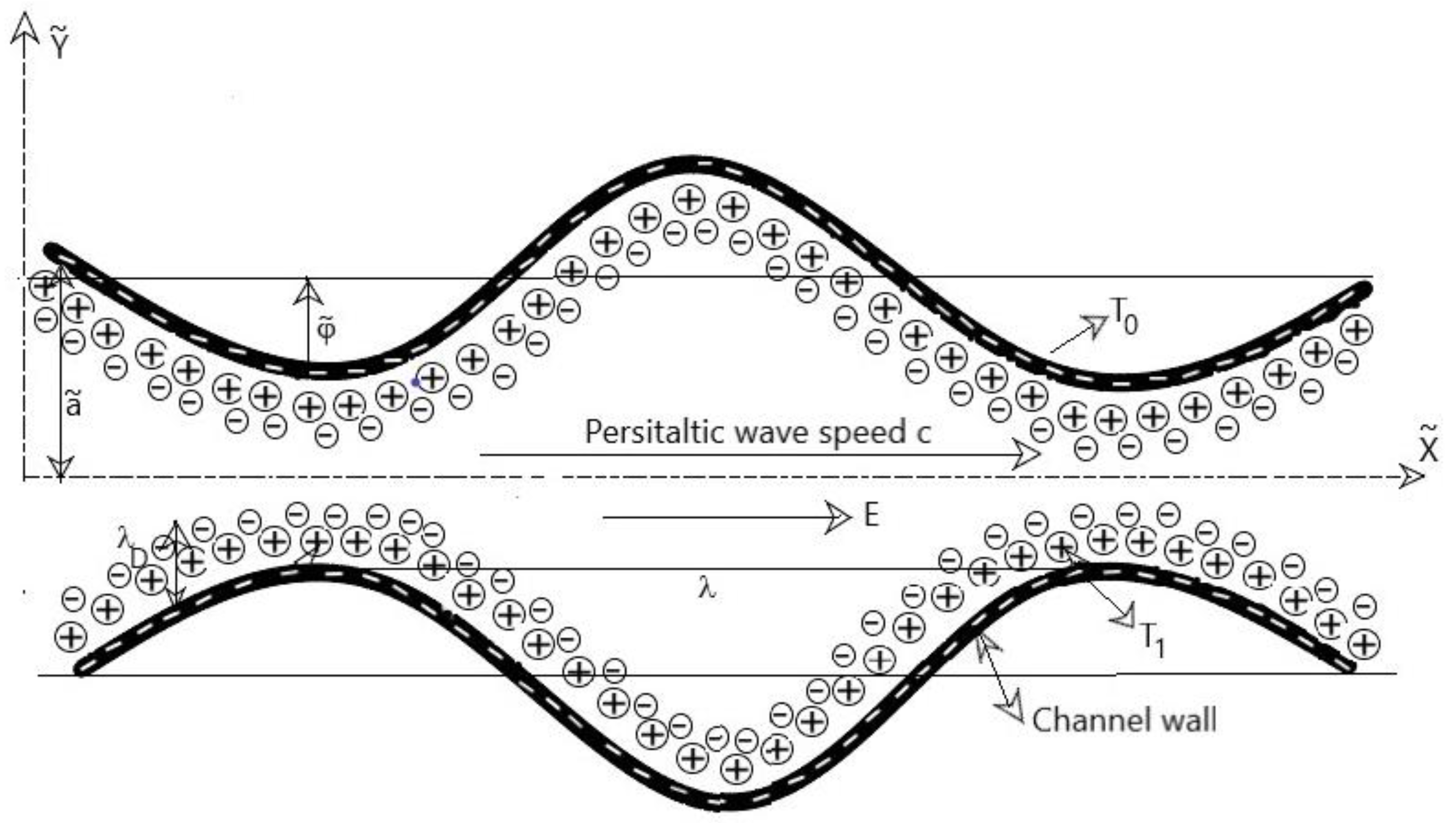
2.1. Flow Regime

Consider two-dimensional peristaltic flow ($\tilde{X},\tilde{Y}$) of an unsteady incompressible Carreau fluid through a wavy micro-channel, shown in Figure 1.

Mathematically, wall deformation in the microchannel is expressed as [23]:

$$\tilde{h}\left(\tilde{X},\tilde{t}\right)=\tilde{a}-\tilde{\phi }{\mathit{cos}}^2\left(\pi \frac{\left(\tilde{X}-c\tilde{t}\right)}{\lambda }\right),$$

(1)

where $\tilde{X},\tilde{h}\left(\tilde{X},\tilde{t}\right),\tilde{\phi },\tilde{a}, c, \tilde{t}$ and $\lambda$ are the axial coordinate, transverse vibration of the wall, wave amplitude, channel’s half width, wave speed, time and wavelength respectively.

2.2. Rheological Carreau Fluid Model

The Cauchy stress tensor for Carreau fluid model is [29]

$$\tilde{\tau }=\eta \left(\tilde{\dot{\gamma }}\right){\tilde{A}}_1,$$

(2)

with

$$\eta \left(\tilde{\dot{\gamma }}\right)={\eta }_{\infty }+\left({\eta }_0-{\eta }_{\infty }\right){\left[1+{\left(\Gamma \tilde{\dot{\gamma }}\right)}^2\right]}^{\left(\frac{n_i-1}{2}\right)},$$

(3)

$${\tilde{A}}_1=\left(\nabla \tilde{\mathit{V}}\right)+{\left(\nabla \tilde{\mathit{V}}\right)}^{\mathrm{T}},\mathrm{where}\tilde{\mathit{V}}=\left[\tilde{U}(\tilde{X},\tilde{Y},\tilde{t}\right), \tilde{V}(\tilde{X},\tilde{Y},\tilde{t}),0]$$

(4)

$$\tilde{\dot{\gamma }}=\sqrt{\frac{1}{2}{\displaystyle \sum }_i{\displaystyle \sum }_{\mathrm{j}}{\tilde{\dot{\gamma }}}_{ij}{\tilde{\dot{\gamma }}}_{ji}}=\sqrt{\frac{1}{2}\Pi }=\sqrt{\frac{1}{2}tr\left({\tilde{A}}_1{}^2\right)},$$

(5)

here $\tilde{\tau },\eta ,\tilde{\dot{\gamma }},{\tilde{A}}_1,{\eta }_0, {\eta }_{\infty },n_i,\Gamma ,\tilde{\mathit{V}}$ and $\Pi$ are the Cauchy stress tensor, shear rate viscosity, shear rate, first Revilin Erickson tensor, zero shear rate viscosity, infinite shear rate viscosity, power law index, material time constant, velocity vector and second invariant tensor (strain rate tensor) respectively. The constitutive Equation (3) for ${\eta }_{\infty }=0$, i.e.,

$$\tilde{\tau }={\eta }_0{\left[1+{\left(\Gamma \tilde{\dot{\gamma }}\right)}^2\right]}^{\left(\frac{n_i-1}{2}\right)}{\tilde{A}}_1.$$

(6)

Note that the Carreau-model with power law index (fluid index $n_i$) expresses the following situations [30]:

(a).

For $n_i=1$ or $\Gamma =0$, Carreau-model reduces to Newtonian fluids.

(b).

For $0<n_i<1$, Carreau-model reduces to pseudoplastic fluids (shear thinning fluids).

(c).

For $n_i>1$, Carreau-model reduces to dilatant fluids (shear thickening fluids).

2.3. Governing Equations and Non-Dimensionalization

Consider the electroosmotic flow (EOF) of an incompressible Carreau fluid altered by means of an externally applied electric field $E_0$ along the length of the micro-channel. Also, energy equation is considered along viscous dissipation. The governing equations for mass, momentum and energy in laboratory frame are [30]:

$$\frac{\partial \tilde{U}}{\partial \tilde{X}}+\frac{\partial \tilde{V}}{\partial \tilde{Y}}=0,$$

(7)

$$\rho \left(\frac{\partial \tilde{U}}{\partial \tilde{t}}+\tilde{U}\frac{\partial \tilde{U}}{\partial \tilde{X}}+\tilde{V}\frac{\partial \tilde{U}}{\partial \tilde{Y}}\right)=-\frac{\partial \tilde{P}}{\partial \tilde{X}}+\left(\frac{\partial {\tilde{\tau }}_{\tilde{X}\tilde{X}}}{\partial \tilde{X}}+\frac{\partial {\tilde{\tau }}_{\tilde{X}\tilde{Y}}}{\partial \tilde{Y}}\right)+{\rho }_e{E}_0,$$

(8)

$$\rho \left(\frac{\partial \tilde{V}}{\partial \tilde{t}}+\tilde{U}\frac{\partial \tilde{V}}{\partial \tilde{X}}+\tilde{V}\frac{\partial \tilde{V}}{\partial \tilde{Y}}\right)=-\frac{\partial \tilde{P}}{\partial \tilde{Y}}+\left(\frac{\partial {\tilde{\tau }}_{\tilde{Y}\tilde{X}}}{\partial \tilde{X}}+\frac{\partial {\tilde{\tau }}_{\tilde{Y}\tilde{Y}}}{\partial \tilde{Y}}\right),$$

(9)

$$\rho c_P\left(\frac{\partial \tilde{T}}{\partial \tilde{t}}+\tilde{U}\frac{\partial \tilde{T}}{\partial \tilde{X}}+\tilde{V}\frac{\partial \tilde{T}}{\partial \tilde{Y}}\right)=k\left(\frac{{\partial }^2\tilde{T}}{\partial {\tilde{X}}^2}+\frac{{\partial }^2\tilde{T}}{\partial {\tilde{Y}}^2}\right)+\left[\frac{\partial \tilde{U}}{\partial \tilde{X}}\left({\tilde{\tau }}_{\tilde{X}\tilde{X}}-{\tilde{\tau }}_{\tilde{Y}\tilde{Y}}\right)+\left(\frac{\partial \tilde{U}}{\partial \tilde{Y}}+\frac{\partial \tilde{V}}{\partial \tilde{X}}\right){\tilde{\tau }}_{\tilde{X}\tilde{Y}}\right].$$

(10)

Here

$${\tilde{\tau }}_{\tilde{X}\tilde{X}}=2{\eta }_0{\left[1+{\left(\Gamma \tilde{\dot{\gamma }}\right)}^2\right]}^{\left(\frac{n_i-1}{2}\right)}\left(\frac{\partial \tilde{U}}{\partial \tilde{X}}\right).$$

(11)

$${\tilde{\tau }}_{\tilde{X}\tilde{Y}}={\eta }_0{\left[1+{\left(\Gamma \tilde{\dot{\gamma }}\right)}^2\right]}^{\left(\frac{n_i-1}{2}\right)}\left(\frac{\partial \tilde{U}}{\partial \tilde{Y}}+\frac{\partial \tilde{V}}{\partial \tilde{X}}\right).$$

(12)

$${\tilde{\tau }}_{\tilde{Y}\tilde{Y}}=2{\eta }_0{\left[1+{\left(\Gamma \tilde{\dot{\gamma }}\right)}^2\right]}^{\left(\frac{n_i-1}{2}\right)}\left(\frac{\partial \tilde{V}}{\partial \tilde{Y}}\right).$$

(13)

$$\tilde{\dot{\gamma }}=\sqrt{2{\left(\frac{\partial \tilde{U}}{\partial \tilde{X}}\right)}^2+{\left(\frac{\partial \tilde{U}}{\partial \tilde{Y}}+\frac{\partial \tilde{V}}{\partial \tilde{X}}\right)}^2+2{\left(\frac{\partial \tilde{V}}{\partial \tilde{Y}}\right)}^2}.$$

(14)

Here $\left(\tilde{U},\tilde{V}\right)$ are velocity components along $\tilde{X}$ and $\tilde{Y}$ direction, respectively. Similarly, $\rho , {\rho }_e, E_0, \tilde{P}, \tilde{T}, k, c_p$ and $\tilde{\dot{\gamma }}$ represents the density of the fluid, electrical charge density, axial electric field, pressure, temperature, thermal conductivity of the fluid, specific heat and strain rate respectively. Also, ${\tilde{\tau }}_{\tilde{X}\tilde{X}}, {\tilde{\tau }}_{\tilde{X}\tilde{Y}}, {\tilde{\tau }}_{\tilde{Y}\tilde{X}}$ and ${\tilde{\tau }}_{\tilde{Y}\tilde{Y}}$ represents the components of extra stress tensor.

Note that the terms on L.H.S of Equation (8) represent inertial forces and on R.H.S first term is due to pressure gradient, second and third terms are surface forces due to linear momentum and last term is body forces due to electrical force per unit volume. Moreover, L.H.S of energy equation characterizes heat transfer due to convection and first two terms on R.H.S represents heat transfer due to diffusion/conduction and the last two terms appearing on R.H.S of Equation (10) represents dissipation due to friction respectively.

To shift from laboratory frame $\left(\tilde{X},\tilde{Y}\right)$ to wave frame $\left(\tilde{x},\tilde{y}\right)$, we define the translational transformation as [8]:

$$\begin{array}{l}\tilde{x}=\tilde{X}-c\widetilde{t,}\tilde{y}=\tilde{Y},\tilde{u}\left(\tilde{x},\tilde{y}\right)=\tilde{U}\left(\tilde{X},\tilde{Y},\tilde{t}\right)-c,\tilde{v}\left(\tilde{x},\tilde{y}\right)=\tilde{V}\left(\tilde{X},\tilde{Y},\tilde{t}\right),\\ \tilde{p}\left(\tilde{x},\tilde{y}\right)=\tilde{P}\left(\tilde{X},\tilde{Y},\tilde{t}\right),T\left(\tilde{x},\tilde{y}\right)=\tilde{T}\left(\tilde{X},\tilde{Y},\tilde{t}\right).\end{array}$$

(15)

For the simplification of governing equations, consider:

$$\begin{array}{c}x=\frac{\tilde{x}}{\lambda },y=\frac{\tilde{y}}{a}, t=\frac{c\tilde{t}}{\lambda }, h=\frac{\tilde{h}}{a}, \phi =\frac{\tilde{\phi }}{a}, p=\frac{\tilde{p}{a}^2}{c{\eta }_0}, m_e=\frac{a_0}{{\lambda }_D}, u=\frac{\tilde{u}}{c}, v=\frac{\tilde{v}}{c\alpha }, \alpha =\frac{a}{\lambda }, n=\frac{\tilde{n}}{n_0},\\ \Theta =\frac{\tilde{T}-T_0}{T_1-T_0},{\lambda }_D=\frac{1}{e{z}_v}\sqrt{\frac{T_0{K}_B\in {\in }_0}{2n_0}}, \mathsf{\varphi }=\frac{e{z}_v}{T_{av}{K}_B}\tilde{\mathsf{\varphi }}, U_{HS}=-\frac{E_x\in {\in }_0}{c\mu },\Psi =\frac{\tilde{\Psi }}{ca}, P_e=\frac{c\lambda }{D},\\ B_r=E_c.P_r, R_e=\frac{\rho ca }{{\eta }_0}, P_r=\frac{{\eta }_0{c}_p}{k}, W_e=\frac{\Gamma c }{a}, {\tau }_{xx}=\frac{\lambda }{{\eta }_{0}c}{\tilde{\tau }}_{\tilde{x}\tilde{x}}, {\tau }_{xy}=\frac{a}{{\eta }_{0}c}{\tilde{\tau }}_{\tilde{x}\tilde{y}}, {\tau }_{yy}=\frac{a}{{\eta }_{0}c}{\tilde{\tau }}_{\tilde{y}\tilde{y}},\\ \dot{\gamma }=\frac{\tilde{\dot{\gamma }}a}{c}, u=\frac{\partial \Psi }{\partial y}, v=-\frac{\partial \Psi }{\partial x},\mathsf{\theta }=\frac{\tilde{\mathrm{Q}}}{ca}, f=\frac{\tilde{\mathrm{q}}}{ca}, E_c=\frac{c^2}{c_p\left(T_1-T_0\right)}.\end{array}$$

(16)

Here, $x$ is the non-dimensional axial coordinate, $y$ is the non-dimensional transverse coordinate, $h$ is the non-dimensional transverse wall’s vibration, $\phi$ is the non-dimensional wave amplitude, $p$ is non-dimensional pressure, $m_e$ is electroosmotic parameter, $\alpha$ is peristaltic wave number, ${\lambda }_D$ is characteristic thickness of EDL/Debye length, $U_{HS}$ is Helmholtz–Smoluchowski velocity, $\Psi$ is non-dimensional stream function, $P_e$ is Peclet number, $B_r$ is Brinkman, $R_e$ is Reynolds number, $P_r$ is Prandtl, $W_e$ is Weissenberg number, $\tau$ is non-dimensional shear stress, $\dot{\gamma }$ is non-dimensional strain rate, $\mathsf{\theta }$ is dimensionless volume flow rate, $E_c$ is Eckert number.

Using Equations (15) and (16) into Equations (7)–(14), after applying a long-wavelength approximation, neglecting higher powers of $\alpha$, and also introducing stream function $\Psi ,$ we get:

$$\frac{\partial p}{\partial x}=\frac{{\partial }^3\Psi }{\partial y^3}+3\left(\frac{n_i-1}{2}\right)W_e{}^2{\left(\frac{{\partial }^2\Psi }{\partial y^2}\right)}^2\frac{{\partial }^3\Psi }{\partial y^3}+m_e{}^2{U}_{HS}\mathsf{\varphi },$$

(17)

$$\frac{\partial p}{\partial y}=0,$$

(18)

$$\frac{{\partial }^2\Theta }{\partial y^2}+B_r\left[{\left(\frac{{\partial }^2\Psi }{\partial y^2}\right)}^2+\left(\frac{n_i-1}{2}\right)W_e{}^2{\left(\frac{{\partial }^2\Psi }{\partial y^2}\right)}^4\right]=0,$$

(19)

After cross differentiation and pressure elimination from the non-dimensional Equations (17) and (18), we get

$$\frac{{\partial }^4\Psi }{\partial y^4}+3\left(\frac{n_i-1}{2}\right)W_e{}^2{\left(\frac{{\partial }^2\Psi }{\partial y^2}\right)}^2\frac{{\partial }^4\Psi }{\partial y^4}+3\left(n_i-1\right)W_e{}^2{\left(\frac{{\partial }^3\Psi }{\partial y^3}\right)}^2\frac{{\partial }^2\Psi }{\partial y^2}+m_e{}^2{U}_{HS}\frac{\partial \mathsf{\Phi }}{\partial y} =0.$$

(20)

2.4. Distribution of Electric Potential

The electric potential $\tilde{\mathsf{\varphi }}$ distribution within a microchannel is given by Poisson-Boltzmann equation [12]:

$${\nabla }^2\tilde{\mathsf{\varphi }}=-\frac{{\rho }_e}{\in {\in }_0}.$$

(21)

Here ${\in }_0{\rho }_e$ and $\in$ represents permittivity of free space, total charge density and relative permittivity of the medium. For electrolyte symmetry $\left(z_v:z_v\right)$ assumption, total charge density ${\rho }_e$ is taken:

$${\rho }_e=-z_{v}e\left({\tilde{n}}^{-}-{\tilde{n}}^{+}\right),$$

(22)

where the cations $\left({\tilde{n}}^{+}\right)$ and anions $\left({\tilde{n}}^{-}\right)$ can be described by number density of Poisson equation:

$${\tilde{n}}^{\pm }={\tilde{n}}_0{e}^{\left(\pm \frac{e{z}_v}{T_{av}{K}_B}\tilde{\mathsf{\varphi }}\right)}.$$

(23)

In the above, $n_0,e, z_v, T_{av}$ and $K_B$ are the number density/bulk concentration, electronic charge, charge balance, average temperature, and Boltzmann constant.

Nernst Planck equation is used to describe $\tilde{\mathsf{\varphi }}$ and determine charge number density [15] as:

$$\left(\frac{\partial {\tilde{n}}_{\pm }}{\partial \tilde{t}}+\tilde{U}\frac{\partial {\tilde{n}}_{\pm }}{\partial \tilde{X}}+\tilde{V}\frac{\partial {\tilde{n}}_{\pm }}{\partial \tilde{Y}}\right)=D_{\pm }\left(\frac{{\partial }^2{\tilde{n}}_{\pm }}{\partial {\tilde{X}}^2}+\frac{{\partial }^2{\tilde{n}}_{\pm }}{\partial {\tilde{Y}}^2}\right)\pm \frac{D_{\pm }{z}_v{}_{\pm }e}{T_0{K}_B}\left(\frac{\partial }{\partial \tilde{X}}\left({\tilde{n}}_{\pm }\frac{\partial \tilde{\mathsf{\varphi }}}{\partial \tilde{X}}\right)+\frac{\partial }{\partial \tilde{Y}}\left({\tilde{n}}_{\pm }\frac{\partial \tilde{\mathsf{\varphi }}}{\partial \tilde{Y}}\right)\right),$$

(24)

where $D_{\pm }, T_0$ and $K_B$ are the ionic species diffusivity, absolute temperature, and Boltzmann constant respectively.

After non-dimensionalization of Equation (24), the nonlinear terms in the Nernst Planck equations are $O\left(P_e{\alpha }^2\right)$, where $P_e=R_e{S}_c$ denotes ionic Peclet number and $S_c$ is the Schmidt number. Using $R_e,P_e ,\alpha \ll 1$, then Equations (21) and (24) becomes:

$$\frac{d^2\mathsf{\varphi }}{d{y}^2}=-m_e{}^2\left(\frac{n_{+}-n_{-}}{2}\right),$$

(25)

$$0=\frac{d^2{n}_{\pm }}{d{y}^2}\pm \frac{\partial }{\partial y}\left(n_{\pm }\frac{\partial \mathsf{\varphi }}{\partial y}\right).$$

(26)

For Equation (26), bulk conditions are

$$n_{\pm }\left(\mathsf{\varphi }=0\right)=1,\frac{\partial n_{\pm }}{\partial y}\left(\frac{\partial \mathsf{\varphi }}{\partial y}=0\right)=0.$$

(27)

Now, first simplifying the Equation (26) subject to the boundary conditions mentioned in Equation (27). This gives the ionic Boltzmann distribution as follows:

$$n_{\pm }=e^{\mp \mathsf{\varphi }}.$$

(28)

Using Equation (28) in Equation (25), we get

$$\frac{d^2\mathsf{\varphi }}{d{y}^2}=m_e{}^2\sinh \mathsf{\varphi }.$$

(29)

As Equation (29) must be modified by a low-zeta potential approach. Using Debye-H$\ddot{u}$ckel linearization approxiamtion [16] i.e., $\sinh \mathsf{\varphi }\approx \mathsf{\varphi }$. Thus, Equation (29) becomes

$$\frac{d^2\mathsf{\varphi }}{d{y}^2}=m_e{}^2\mathsf{\varphi },$$

(30)

subject to the boundary conditions

$$\frac{\partial \mathsf{\varphi }}{\partial y}\left(0\right)=0,\mathsf{\varphi }\left(h\right)=1,$$

(31)

whereas the analytical solution of electric potential $\mathsf{\varphi }$ is obtained

$$\mathsf{\varphi }=\frac{\cosh \left(m_{e}y\right)}{\cosh \left(m_{e}h\right)}.$$

Here, $m_e$ is the electroosmotic parameter.

2.5. Boundary Conditions and Volume Flow Rate

If we choose $\Psi =0$ along the centerline ($y=0$), then the value of stream function at the wall ($y=h$) is $\Psi =f$ [9]. For the simplification of governing Equations (17)–(19) in wave frame, the dimensionless boundary conditions are:

$$\frac{d^2\Psi }{d{y}^2}=0, \Psi =0, \Theta =0, \mathrm{at}y=0,$$

(32a)

$$\frac{\partial \Psi }{\partial y}=-1, \Psi =f, \Theta =1,\mathrm{at}y=h\left(x,t\right).$$

(32b)

Here no slip conditions are at the walls and symmetry conditions along centerline of channel. Moreover, the non-dimensional time average flow rate $f$ in the moving frame is connected to the non-dimensional time average flow rate $\mathsf{\theta }$ in the fixed frame as:

$$\mathsf{\theta }=f+1-\frac{\phi }{2},$$

(33)

where $f={{\displaystyle \int }}_0^h\frac{\partial \Psi }{\partial y}dy=\Psi \left(\mathrm{h}\right)-\Psi \left(0\right)$ at $y=h\left(x,t\right)=1-\phi {\mathit{cos}}^{2}x.$

3. Solution Methodology

3.1. Perturbation/Series Solution

Equation (20) is a nonlinear PDE and its closed form solution is not possible. Therefore, it can be solved analytically by perturbation technique about $W_e$ parameter, by expanding $\Psi$, $\Theta$, $dp/dx$ and $f$ in the following forms [25]:

$$\Psi ={\Psi }_0+W_e{}^2{\Psi }_1+O{\left(W_e{}^2\right)}^2,$$

(34)

$$\Theta ={\Theta }_0+W_e{}^2{\Theta }_1+O{\left(W_e{}^2\right)}^2,$$

(35)

$$\frac{dp}{dx}=\frac{d{p}_0}{dx}+\frac{W_e{}^{2}d{p}_1}{dx}+O{\left(W_e{}^2\right)}^2,$$

(36)

$$f=f_0+W_e{}^2{f}_1+{\left(W_e{}^2\right)}^2.$$

(37)

3.2. Zero Order System ${\left(W_e{}^2\right)}^0$

$$\frac{{\partial }^4{\Psi }_0}{\partial y^4}+m_e{}^2{U}_{HS}\frac{\partial \mathsf{\varphi }}{\partial y}=0,$$

(38)

$$\frac{{\partial }^2{\Theta }_0}{\partial y^2}+B_r{\left(\frac{{\partial }^2{\Psi }_0}{\partial y^2}\right)}^2=0,$$

(39)

$$\frac{\partial p_0}{\partial x}=\frac{{\partial }^3{\Psi }_0}{\partial y^3}+m_e{}^2{U}_{HS}\mathsf{\varphi },$$

(40)

subject to

$$\frac{{\partial }^2{\Psi }_0}{\partial y^2}=0,{\Psi }_0=0,{\Theta }_0=0 at y=0, \frac{\partial {\Psi }_0}{\partial y}=-1,{\Psi }_0=f_0,{\Theta }_0=1 at y=\mathrm{h}.$$

(41)

3.3. First Order System ${\left(W_e{}^2\right)}^1$

$$\frac{{\partial }^4{\Psi }_1}{\partial y^4}+3\left(\frac{n_i-1}{2}\right){\left(\frac{{\partial }^2{\Psi }_0}{\partial y^2}\right)}^2\frac{{\partial }^4{\Psi }_0}{\partial y^4}+3\left(n_i-1\right){\left(\frac{{\partial }^3{\Psi }_0}{\partial y^3}\right)}^2\frac{{\partial }^2{\Psi }_0}{\partial y^2}=0,$$

(42)

$$\frac{{\partial }^2{\Theta }_1}{\partial y^2}+B_r\left[2\left(\frac{{\partial }^2{\Psi }_0}{\partial y^2}\right)\left(\frac{{\partial }^2{\Psi }_1}{\partial y^2}\right)+\left(\frac{n_i-1}{2}\right){\left(\frac{{\partial }^2{\Psi }_0}{\partial y^2}\right)}^2\right]=0,$$

(43)

$$\frac{\partial p_1}{\partial x}=\frac{{\partial }^3{\Psi }_1}{\partial y^3}+3\left(\frac{n_i-1}{2}\right){\left(\frac{{\partial }^2{\Psi }_0}{\partial y^2}\right)}^2\frac{{\partial }^3{\Psi }_0}{\partial y^3},$$

(44)

subject to

$$\frac{{\partial }^2{\Psi }_1}{\partial y^2}=0,{\Psi }_1=0,{\Theta }_0=0 at y=0, \frac{\partial {\Psi }_1}{\partial y}=0,{\Psi }_1=f_1,{\Theta }_0=0 at y=\mathrm{h}.$$

(45)

The solutions for zero and first order system is defined in Appendix A. By putting the zero and first order solution of stream function $\Psi$, temperature $\Theta$ and pressure gradient $dp/dx$ in the Equations (34)–(36) we get the final first order solution for $\Psi , \Theta$ and $dp/dx$.

The dimensionless pressure rise per wavelength $\mathsf{\Delta }{P}_{\lambda }$ is as follows:

$$\mathsf{\Delta }{P}_{\lambda }={{\displaystyle \int }}_0^1\frac{\partial p}{\partial x}dx,$$

(46)

the above expression is also solved by using final first order solution of $dp/dx.$

The rate of heat transfer (Nusselt number $N_u$) is defined as:

$$N_u= \frac{\partial h}{\partial x}\frac{\partial \Theta }{\partial y}{|}_{y = h\left(x\right)}.$$

(47)

4. Computational Results and Discussion

The purpose here is to study the physical feature of the different parameters (Weissenberg number $W_e$, power law index/fluid index $n_i$, electroosmotic parameter $m_e$, Helmholtz–Smoluchowski velocity $U_{HS}$, volume flow rate $\mathsf{\theta }$ and Brinkman number $B_r$) on the flow quantities such as axial velocity $u$, pressure gradient $dp/dx$, pressure rise $\mathsf{\Delta }{P}_{\lambda }$, streamlines and temperature $\theta$. Solutions are illustrated in the Figures 2–10.

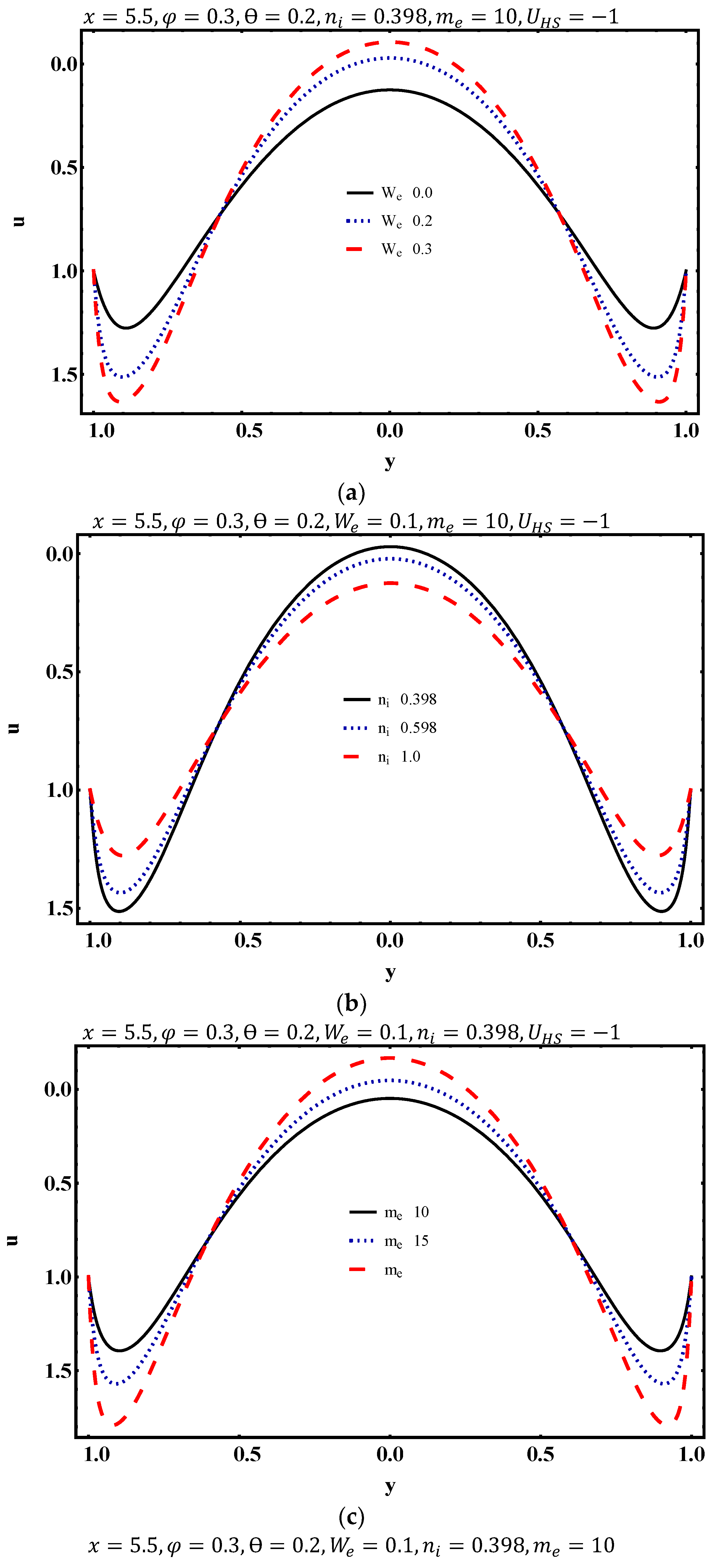
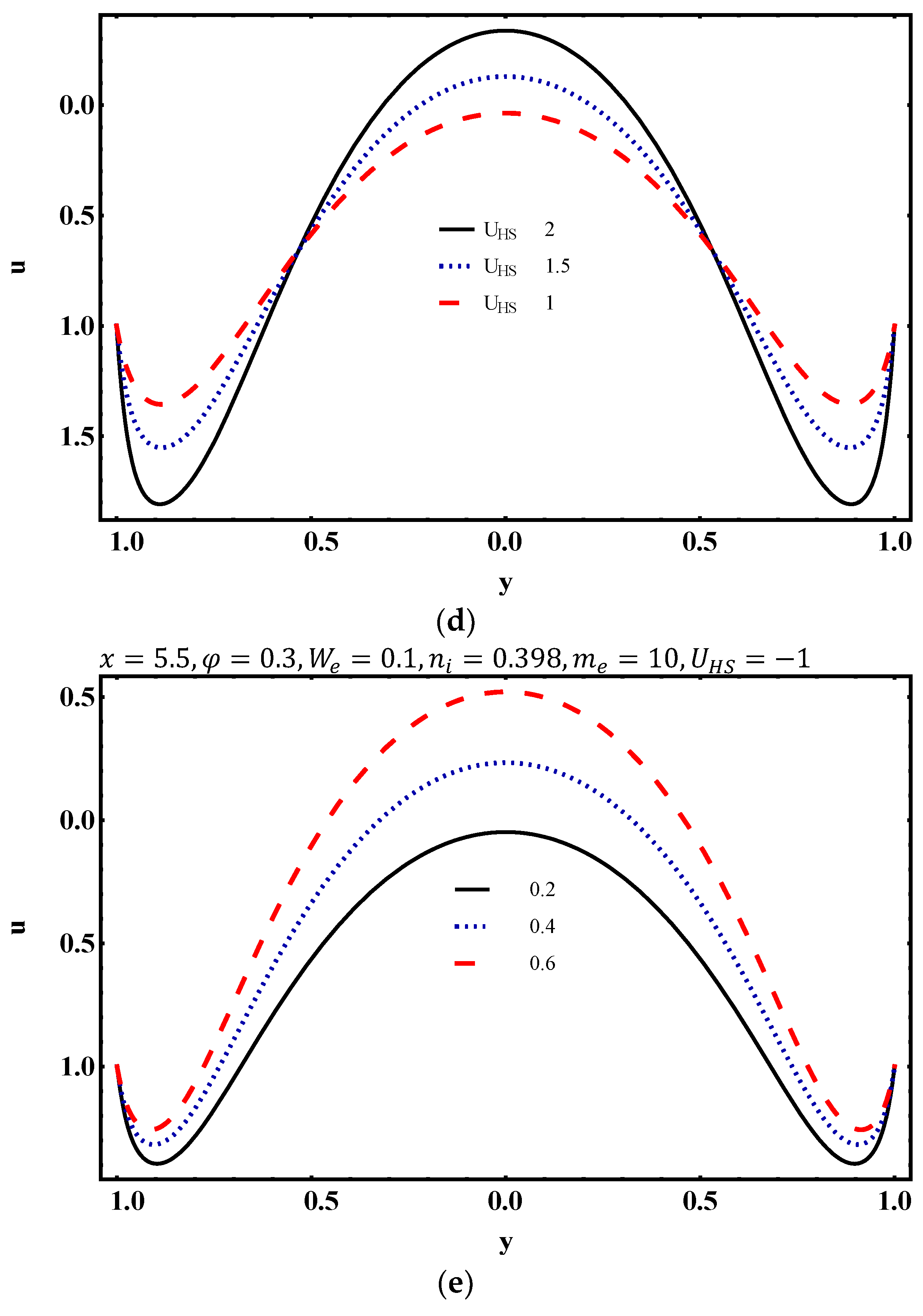
4.1. Flow Characteristics

The velocity profile under the stimulus of Weissenberg number $W_e$, power law index/fluid index $n_i$, electroosmotic parameter $m_e$, Helmholtz–Smoluchowski velocity $U_{HS}$ and volume flow rate $\mathsf{\theta }$ is shown in Figure 2a–e. Figure 2a,b illustrates the variation of axial velocity for increasing values of $W_e$ and $n_i$. It is predicted that the magnitude of $u$ increases as $W_e$ increases and decreases as $n_i$ increases. But opposite behavior is witnessed near the channel walls. Because, $W_e$ is directly proportional to the time constant and inversely proportional to the width of the channel. Figure 2c demonstrates that electroosmotic parameter $m_e$ enhances the magnitude of $u$ i.e., magnitude of $u$ increases as $m_e$ increases at centerline of the channel. Figure 2d reveals that $u$ decreases for higher values of $U_{HS}$ in the center of channel, whereas opposite behavior is noticed near walls. Since, $U_{HS}$ physically interprets that fluid velocity reduces with greater EDL thickness. Figure 2e displays the impact of u with respect to $\mathsf{\theta }$. It has also been noticed that change in $\mathsf{\theta }$ increases the $u$ because flow rate is directly proportional to the fluid velocity. We observed that our study is consistent with previous results [26].

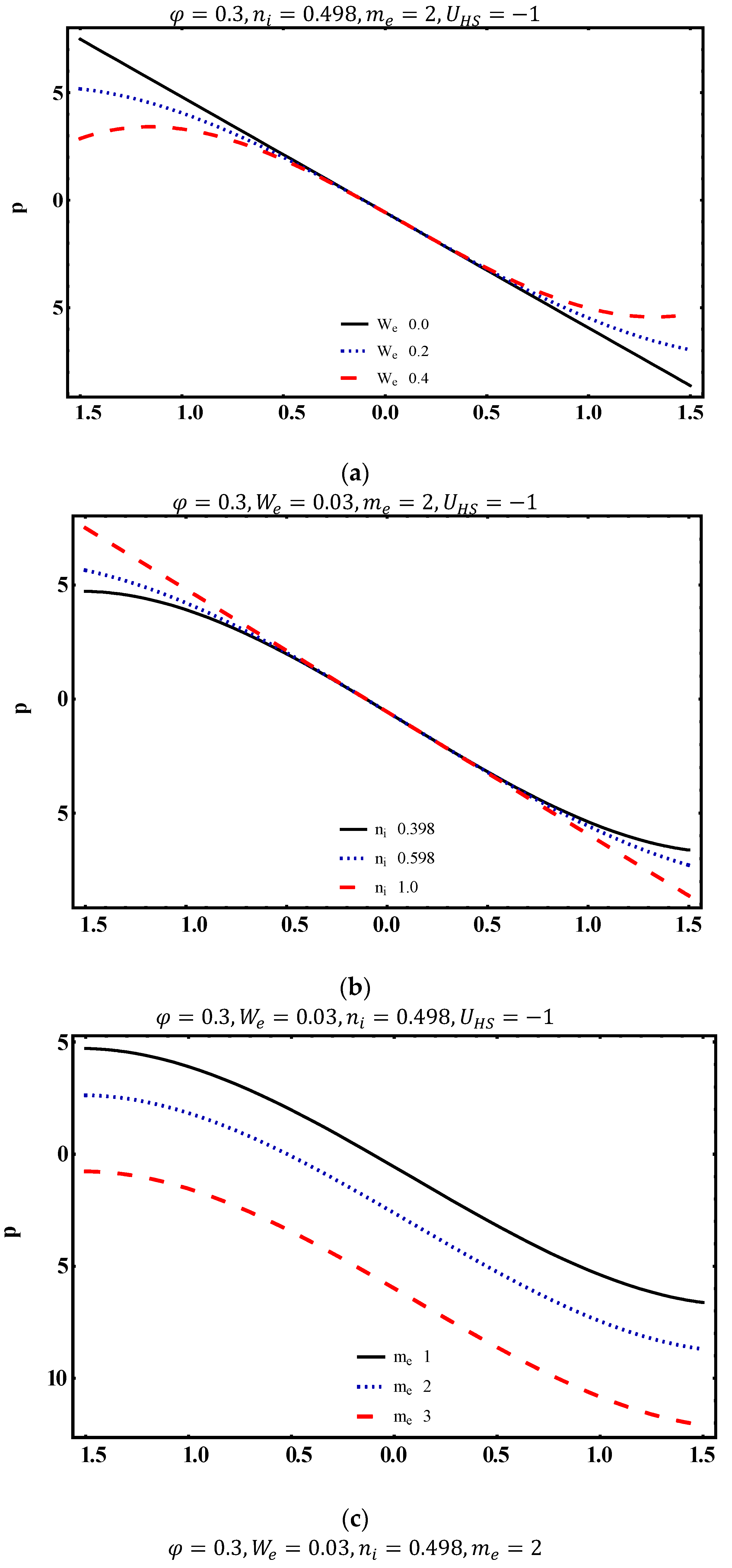
4.2. Pumping Characteristics

The characteristic feature of peristalsis is pumping. The pumping characteristic can be scrutinized in the form of $\mathsf{\Delta }{P}_{\lambda }$ versus $\mathsf{\theta },$ illustrated in Figure 3a–d. Pumping action divides the whole region into the four segments: pumping region (adverse pressure gradient $\mathsf{\Delta }{P}_{\lambda }>0$, Positive pumping $\mathsf{\theta }>0$), backward/retrograde pumping ($\mathsf{\Delta }{P}_{\lambda }>0$,$\mathsf{\theta }<0$), augmented pumping (favorable pressure gradient $\mathsf{\Delta }{P}_{\lambda }<0$, Positive pumping $\mathsf{\theta }>0$) and free pumping ($\mathsf{\Delta }{P}_{\lambda }=0$). Figure 3a elucidates the $\mathsf{\Delta }{P}_{\lambda }$ against $\mathsf{\theta }$ for different values of $W_e$. It is seen that pumping decreases as $W_e$ increases in the pumping region ($\mathsf{\Delta }{P}_{\lambda }>0$). But in co-pumping ($\mathsf{\Delta }{P}_{\lambda }<0$), the pumping increases as $W_e$ increases. For free pumping ($\mathsf{\Delta }{P}_{\lambda }=0$), curves coincide i.e., there is no difference between Carreau fluid and Newtonian fluid. Figure 3b portrays the $\mathsf{\Delta }{P}_{\lambda }$ against $\mathsf{\theta }$ for different values of $n_i$. It reveals that pumping enhances as $n_i$ increases in the pumping region ($\mathsf{\Delta }{P}_{\lambda }>0$). But in the case is reverse in co-pumping ($\mathsf{\Delta }{P}_{\lambda }<0$) i.e., the pumping decreases as $n_i$ increases. Figure 3c depicts that $\mathsf{\Delta }{P}_{\lambda }$ decreases as $m_e$ increases. It physically declares that formation of EDL on charged surface opposes the Carreau fluid flow. Furthermore, Figure 3d depicts $\mathsf{\Delta }{P}_{\lambda }$ decreases as $U_{HS}$ increases. Here pumping is modulated in presence of electric field. It is noticed that because of $U_{HS}$, the relation between $\mathsf{\Delta }{P}_{\lambda }$ against $\mathsf{\theta }$ becomes linear.

The distribution of pressure gradient is plotted in Figure 4a–e for various values of Weissenberg number $W_e$, fluid index $n_i$, electroosmotic parameter $m_e$, Helmholtz–Smoluchowski velocity $U_{HS}$ and volume flow rate $\mathsf{\theta }$. Figure 4a highlights that by increasing the $W_e,$ magnitude of pressure gradient $dp/dx$ increase. As Weissenberg number $W_e$, is the inversely proportional to channel width. So, lesser the channel width, large amount of pressure is needed to maintain the flux to pass through it. Figure 4b depicts that by increasing the $n_i,$ magnitude of $dp/dx$ decreases. Figure 4c shows that by raising the values of $m_e,$ $dp/dx$ decreases. Figure 4d illustrates that the magnitude of $dp/dx$ increases as $U_{HS}$ increases. Also, Figure 4e presents that by increasing the values of $\mathsf{\theta },$ $dp/dx$ decreases. Because there is an inverse relationship between $dp/dx$ and $\mathsf{\theta }$.

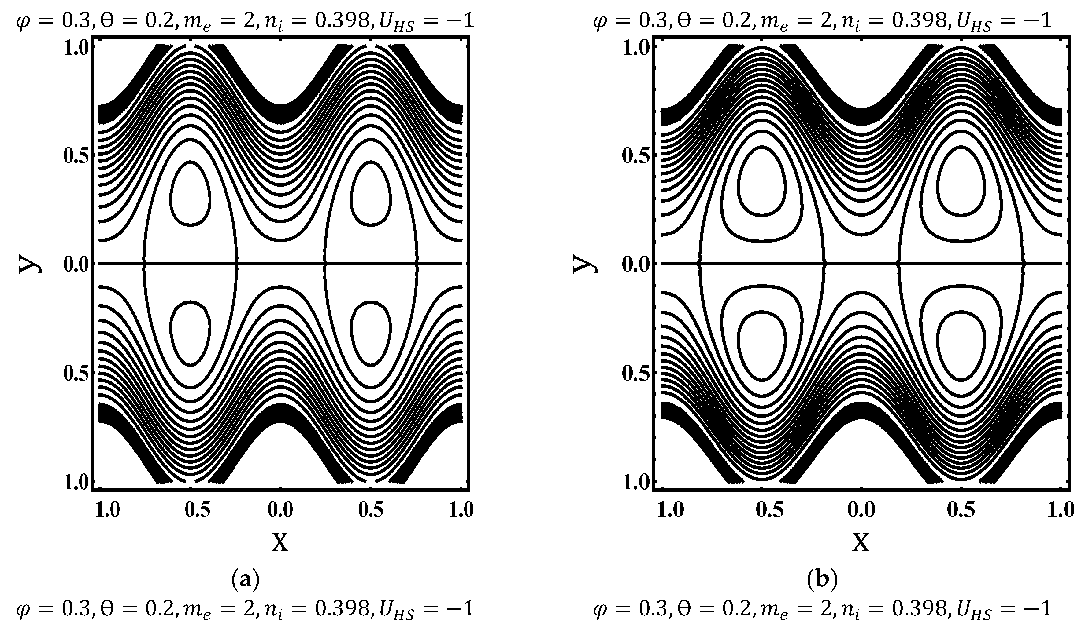
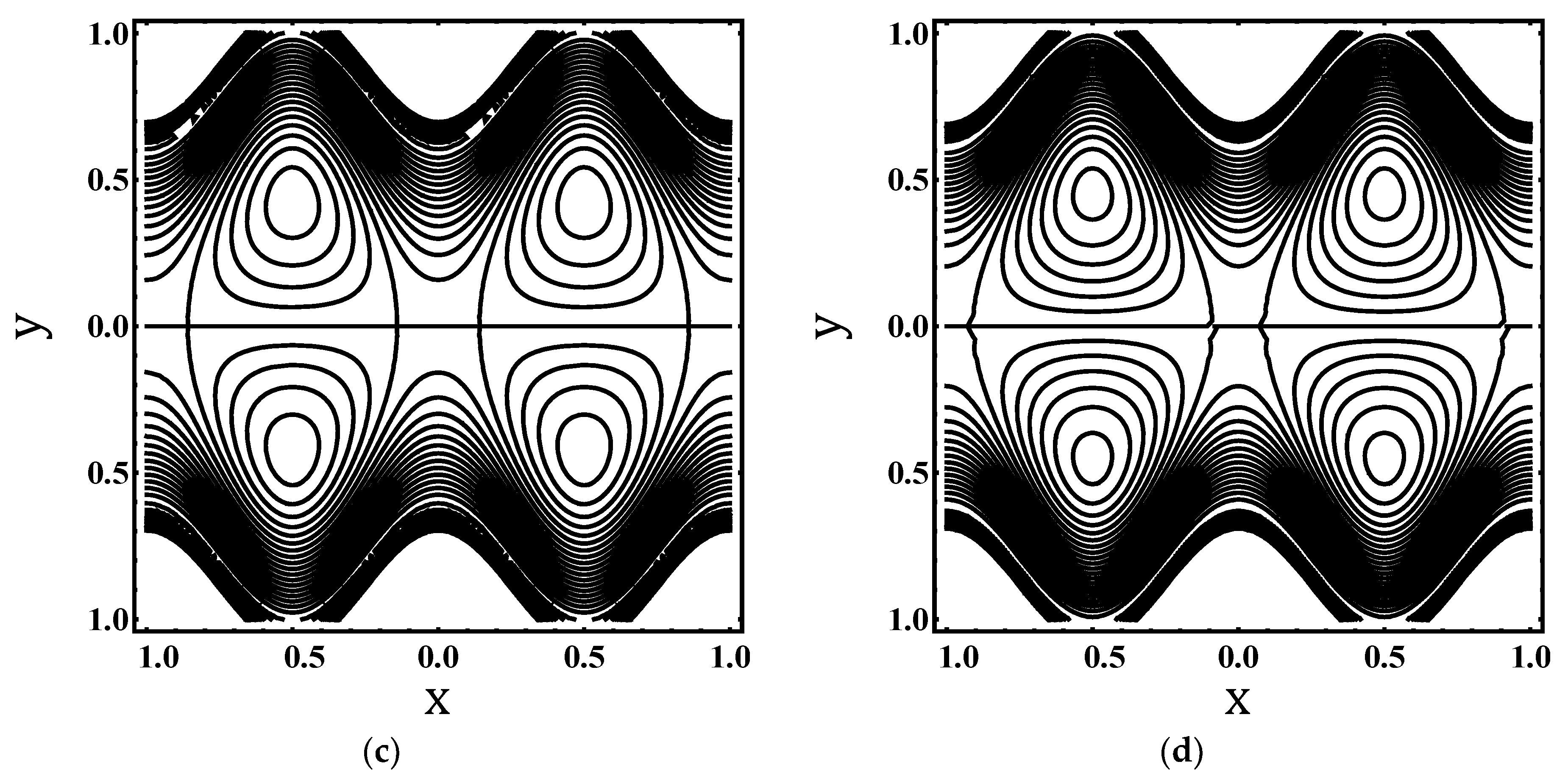
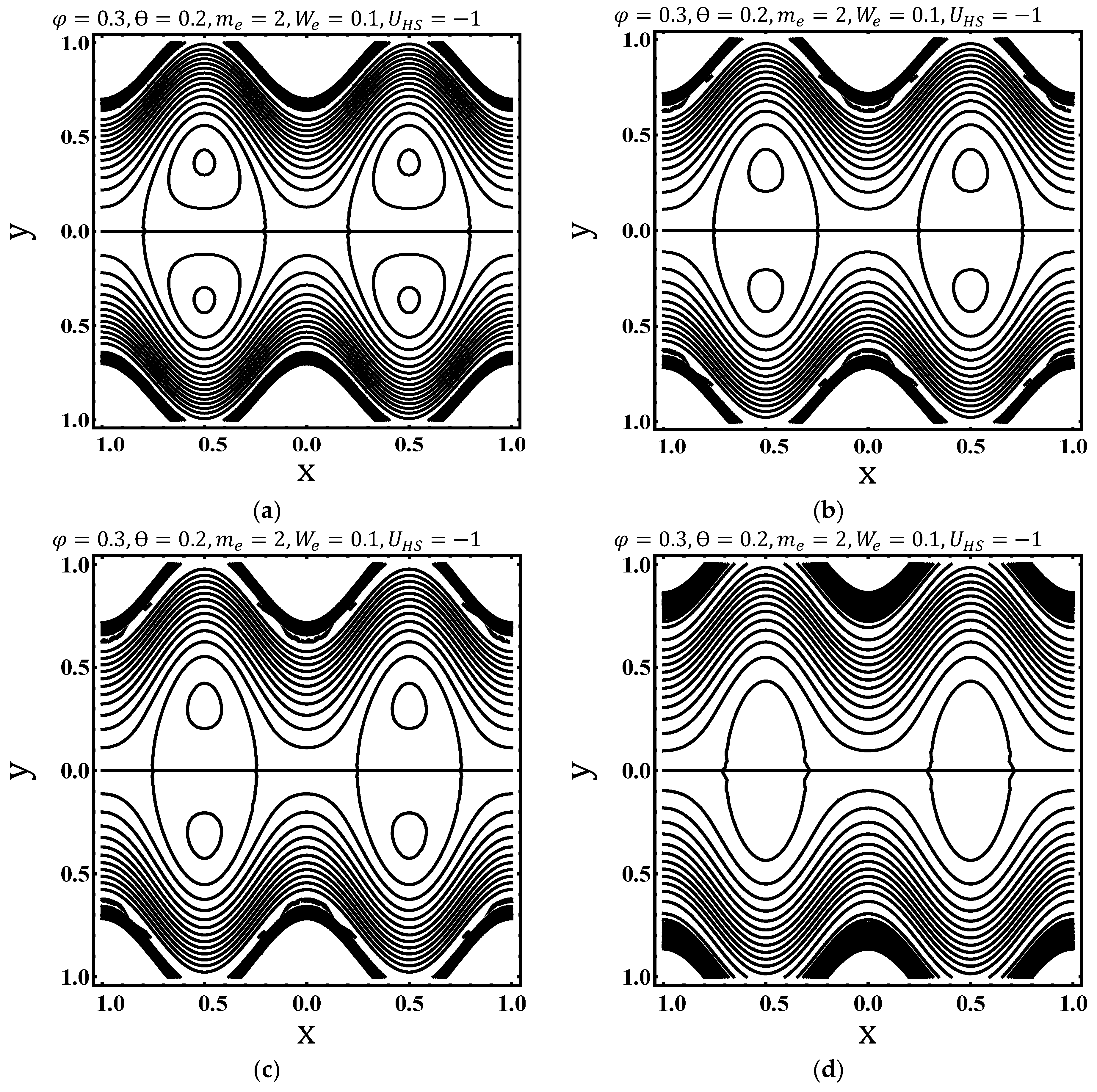
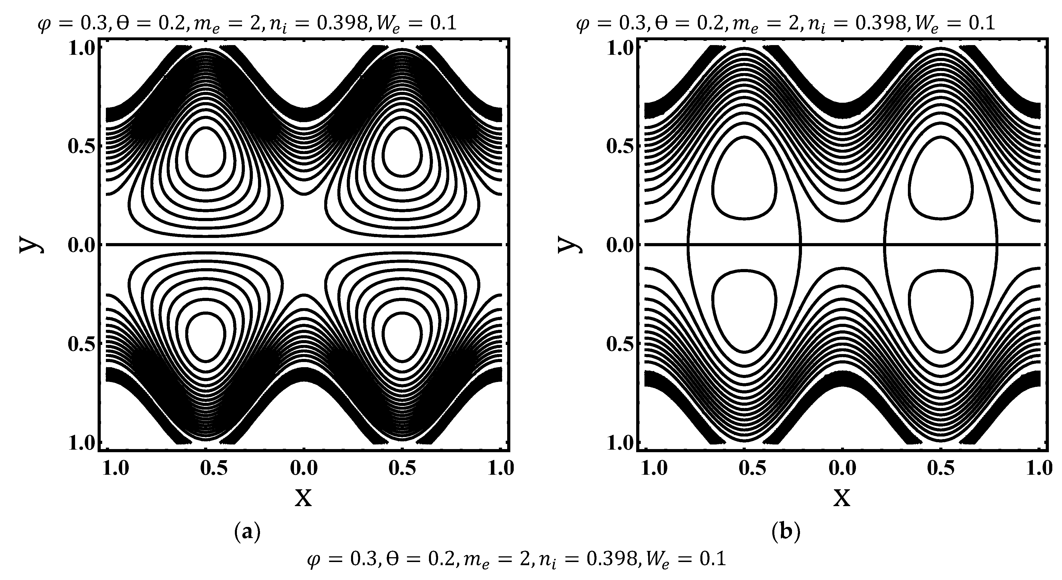
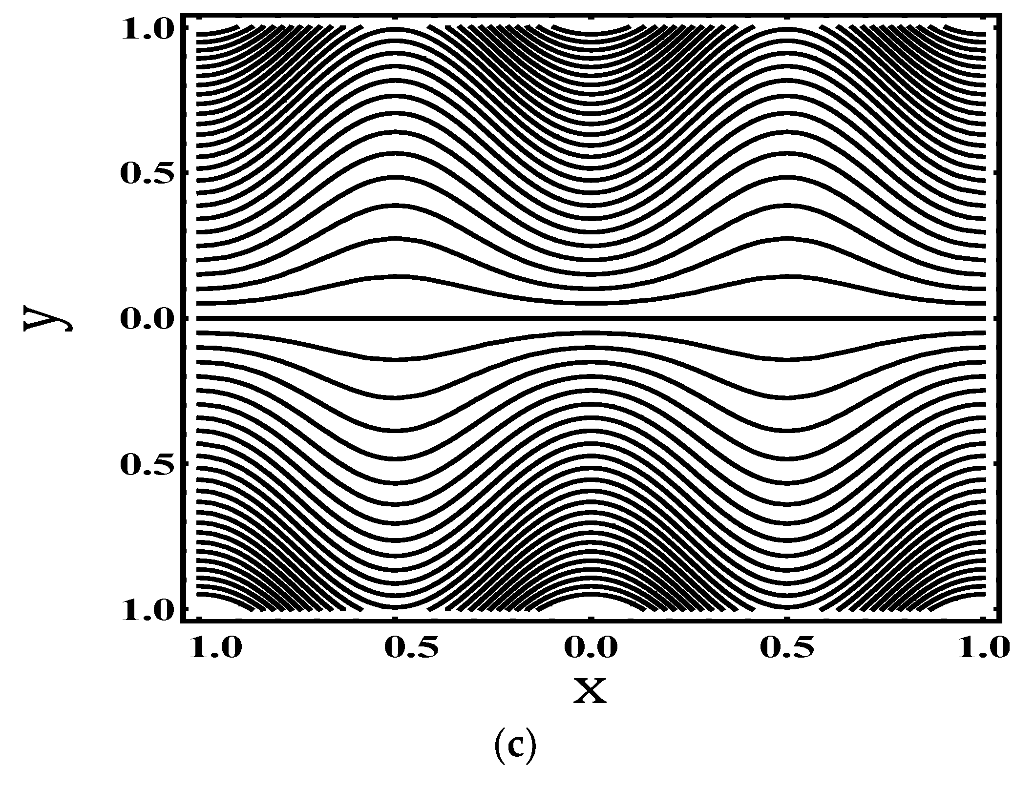
4.3. Trapping Characteristics

Figure 5, Figure 6, Figure 7 and Figure 8 displays streamline structural changes for different of fluid index $n_i$, Weissenberg number $W_e,$ electroosmotic parameter $m_e$, and Helmholtz–Smoluchowski velocity $U_{HS}$. Figure 5a–d depict streamline structure for increasing values of $W_e$. It is seen that the size of enclosed bolus increases with rise in $W_e$. Since, $W_e$ is directly proportional to velocity, so no. of trapped bolus increases as velocity increases. Similarly, Figure 6a–d visualize the streamline structure for different values of $n_i$. It is observed that the size of trapped bolus decreases with rise in $n_i$. Figure 7a–d show that the number of trapped bolus grows with rise in electroosmotic parameter $m_e$. It inspects that as the $m_e$ increases, the tapping bolus strongly appears in EDL. Figure 8a–d depict streamline structure for different values of $U_{HS}$. It demonstrates that the accumulation of streamline decreases with increase in $U_{HS}$. Since $U_{HS}$ is directly proportional to electric field. Thus, stronger $U_{HS}$ means stronger the external electric field, which strongly effects the bolus formation.

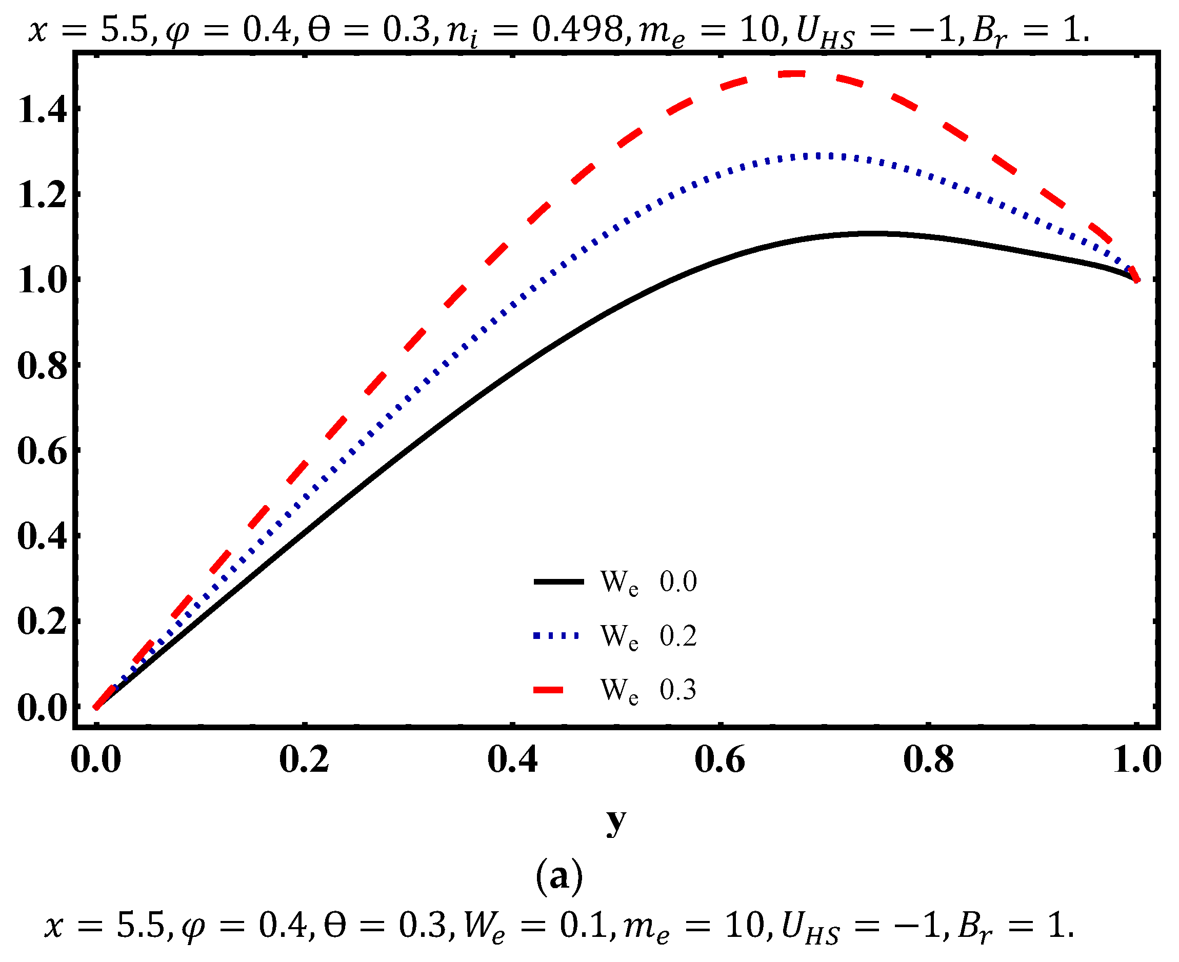
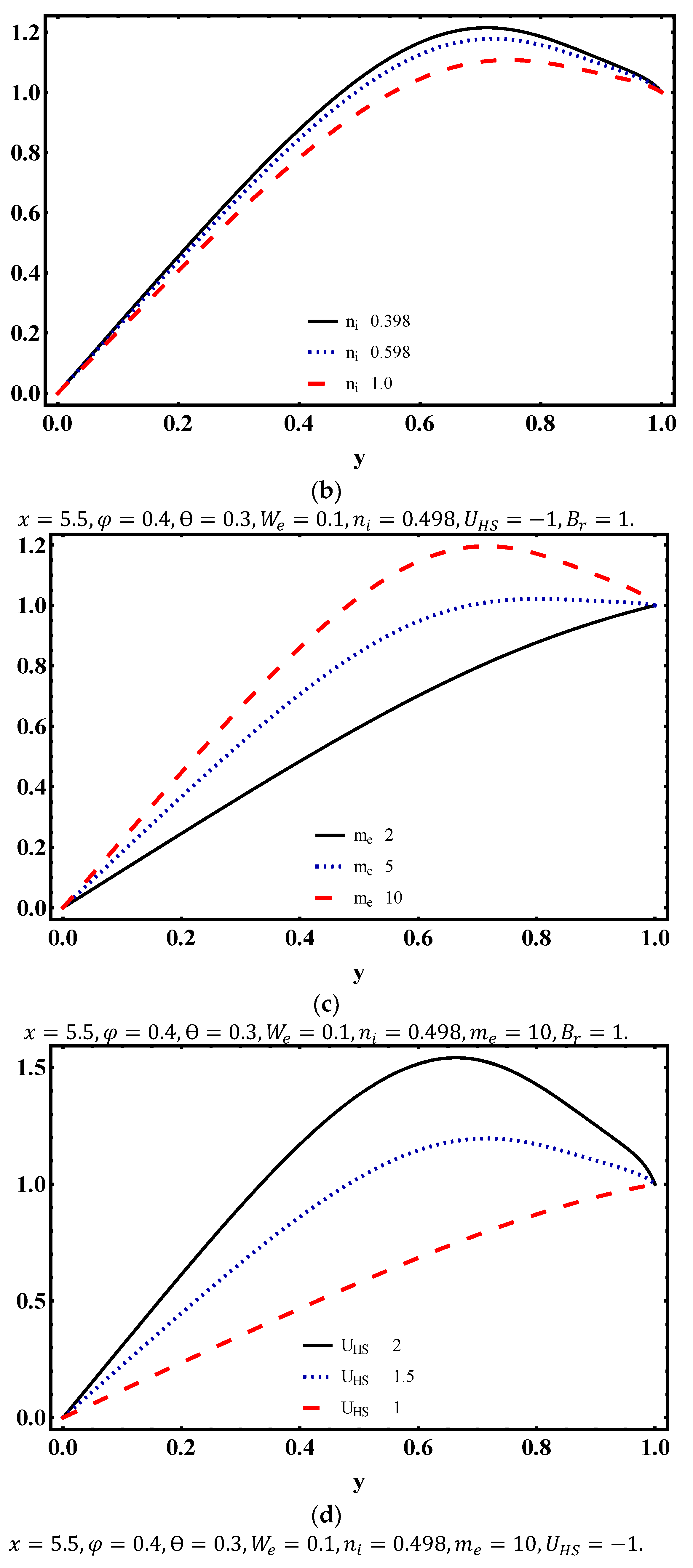
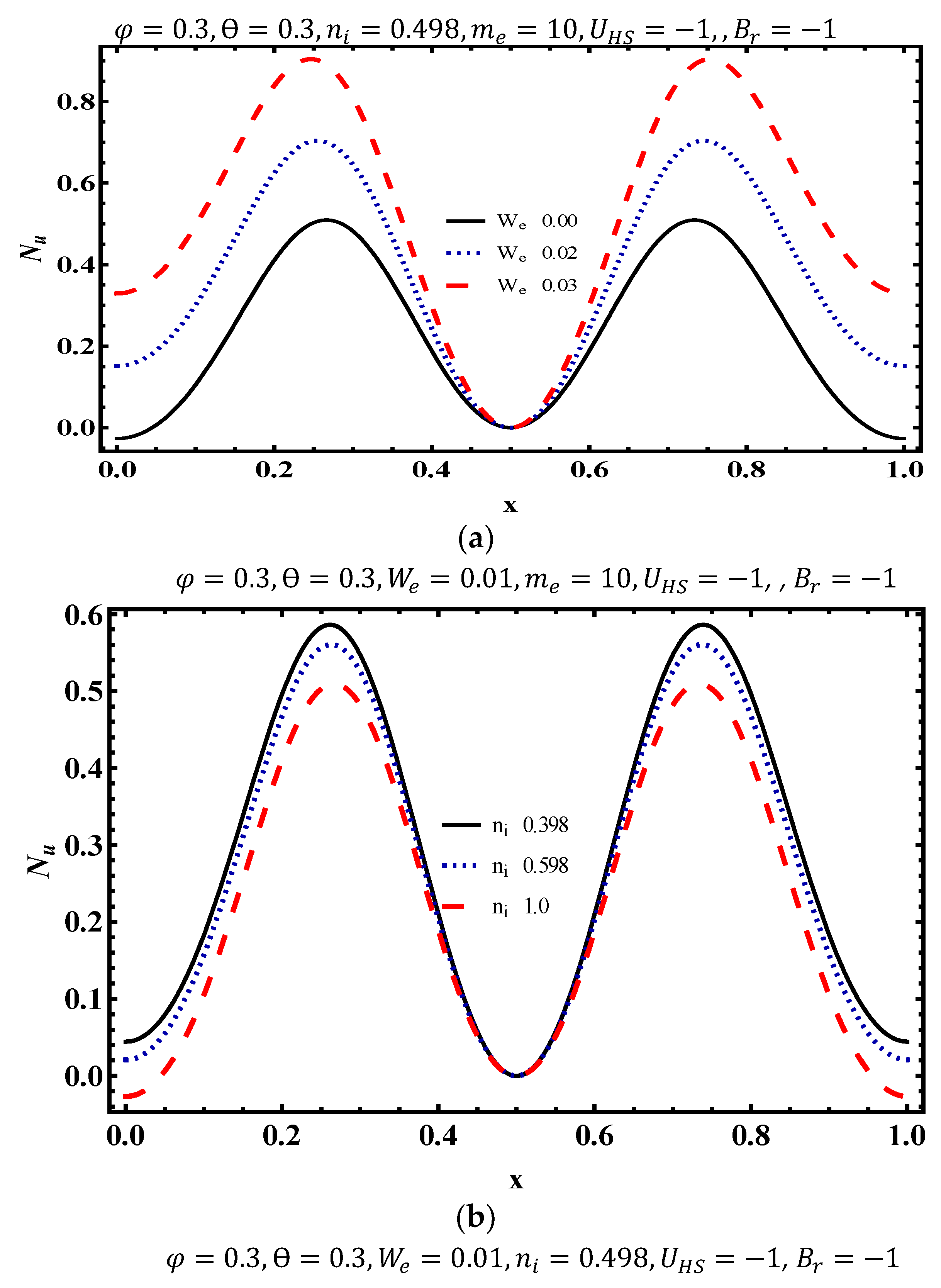
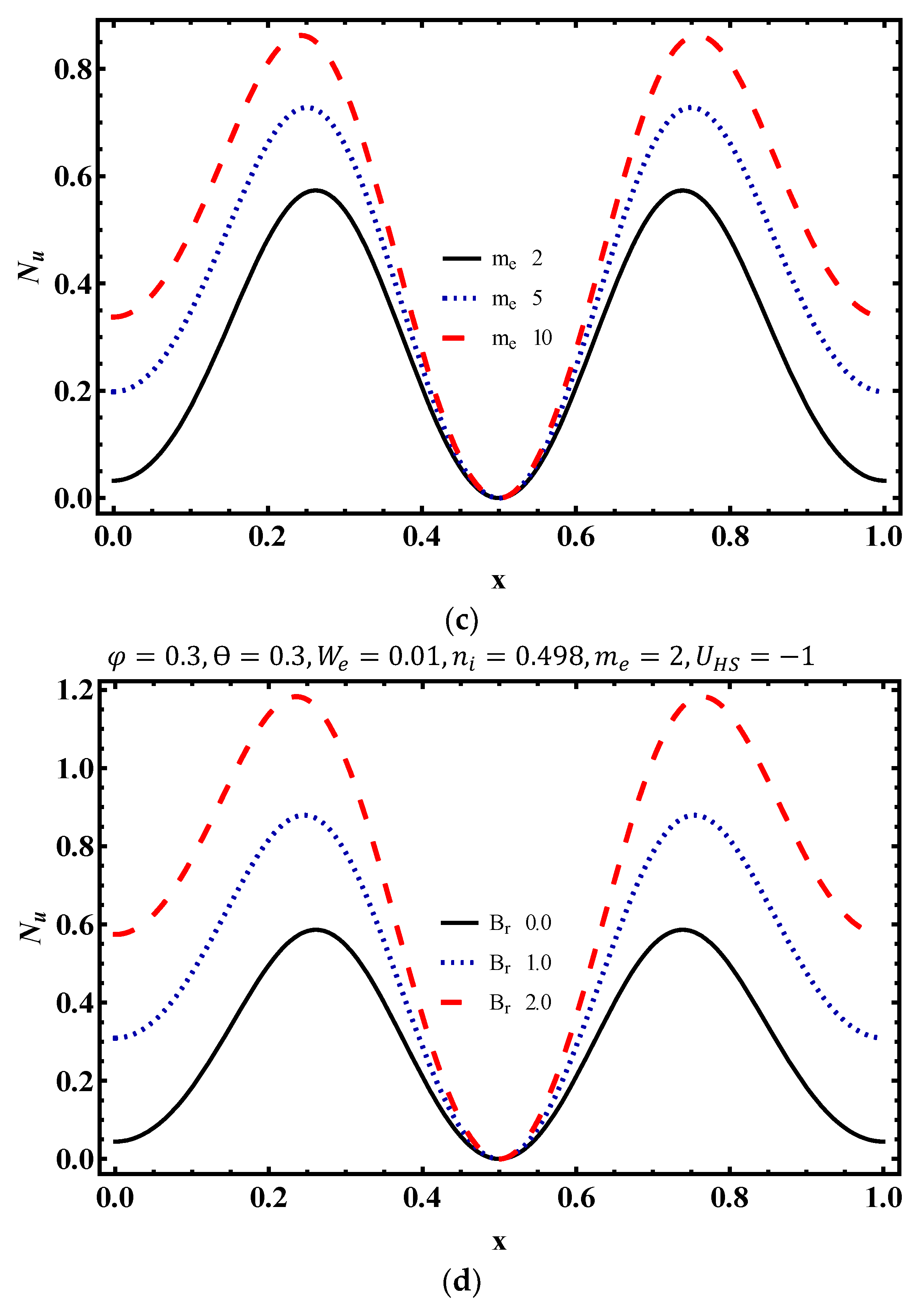
4.4. Temperature Characteristics

In this section, we analyzed the effect of Weissenberg number $W_e$, power law index/fluid index $n_i$, electroosmotic parameter $m_e$, Helmholtz–Smoluchowski velocity $U_{HS}$ and Brinkman number $B_r$ on heat transfer characteristics. Figure 9a discloses the various values of $W_e$, for temperature distribution $\theta .$ It examines that $\theta$ enhances for more values of $W_e.$ Since $W_e$ is directly proportional to velocity, so for higher values of velocity, temperature will be higher. Temperature variation against various values of $n_i$ can be observed in Figure 9b. It portrays that $\theta$ decreases as $n_i$ increases. Figure 9c displays that temperature increases very quickly by increasing the values of electroosmotic parameter $m_e$. Therefore, decrease in EDL produces rise in $\theta$ remarkably. Figure 9d shows the effects of Helmholtz–Smoluchowski velocity $U_{HS}$ on $\theta$. It signifies that for more values of $U_{HS}$, $\theta$ declines. Figure 9e demonstrates the impact of $B_r$ on $\theta$ i.e., $\theta$ increases for more values of $B_r$. In other words, for higher values of $B_r$, lower be the heat conduction due to viscous dissipation. Hence, temperature increases.

Figure 10a–d represents the variation of Nusselt number $N_u$ for various values of Weissenberg number $W_e$, fluid index $n_i$, electroosmotic parameter $m_e$ and Brinkman number $B_r$. Figure 10a highlights that by increasing the $W_e,$ magnitude of Nusselt number $N_u$ increase. Figure 10b depicts that by increasing the $n_i,$ magnitude of $N_u$ decreases. Figure 10c shows that by raising the values of $m_e,$ $N_u$ increases. Also, Figure 10d illustrates that the magnitude of $N_u$ increases as $B_r$ increases.

5. Concluding Remarks

A mathematical model of electroosmotic peristaltic transport for Carreau fluid through wavy microchannel is established. Effect of viscous dissipation is likewise considered in this model. Debye Hückel linearization and long wavelength assumptions are used. The solution (analytical) of axial velocity, pressure gradient, pressure rise, temperature and stream function are presented by using a perturbation technique. The main conclusions from the present analysis are:

• The axial velocity increases with higher values of Weissenberg number, electroosmotic parameter and averaged time flow rate.
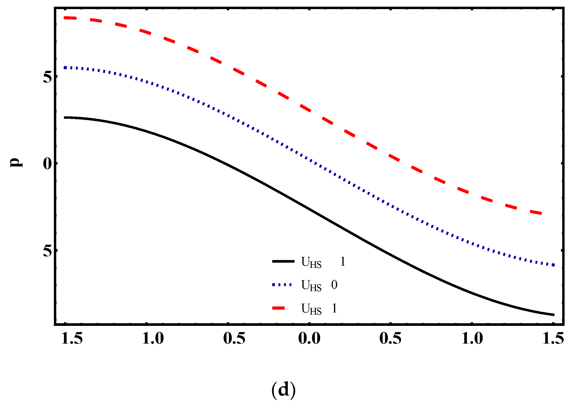
• The magnitude of pressure rise decreases in the pumping region with the increase of Weissenberg number and electroosmotic parameter.
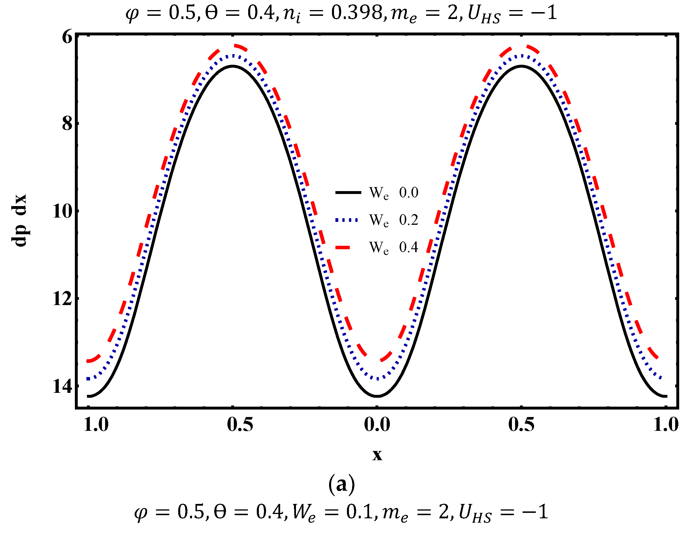
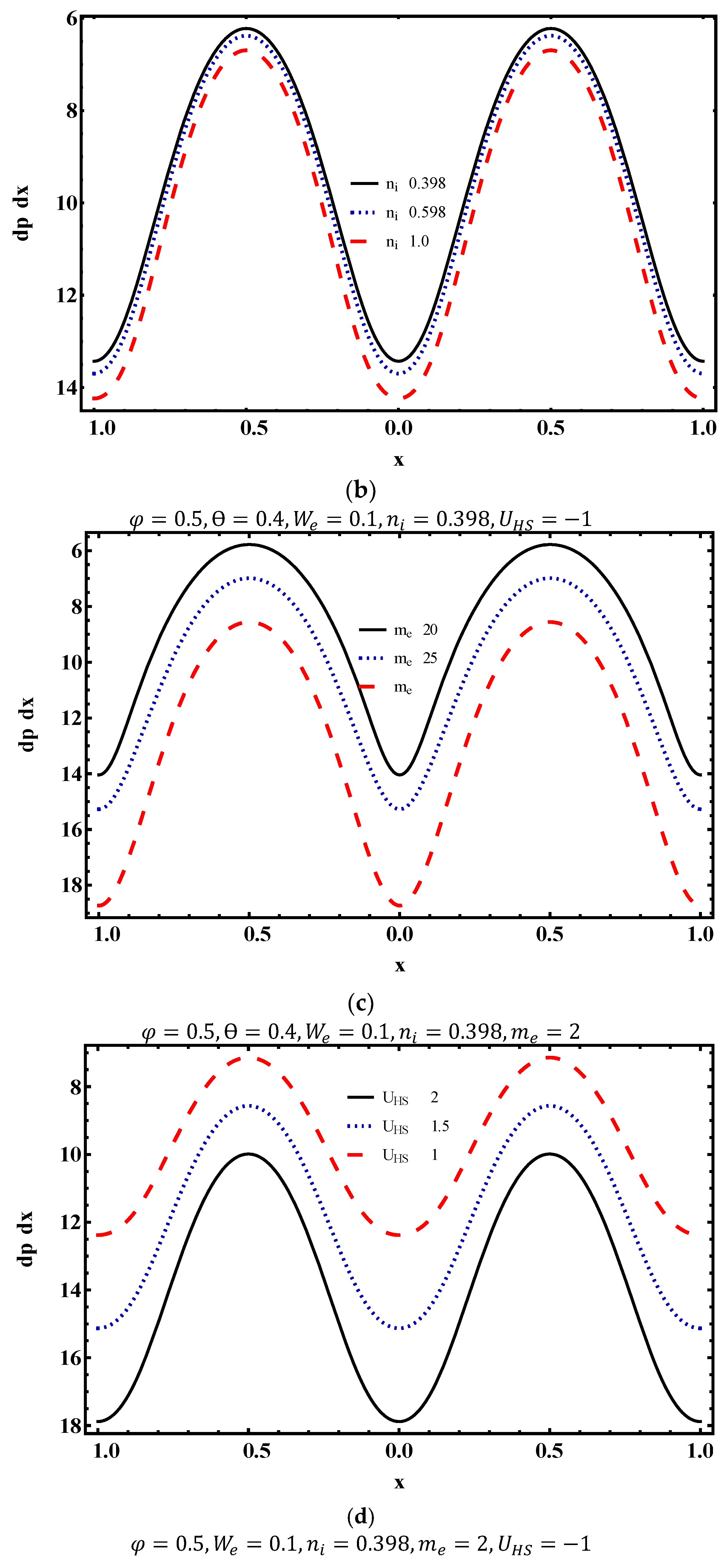
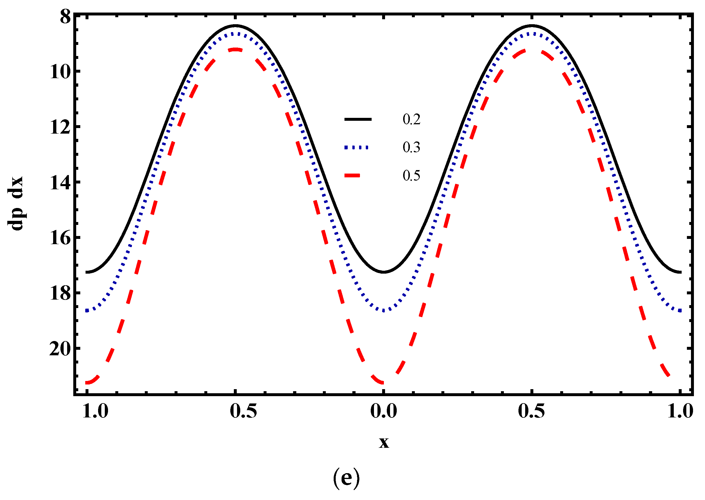
• Pressure gradient is more for Weissenberg number and Helmholtz–Smoluchowski velocity and declines for fluid index, electroosmotic parameter and averaged time flow rate.
• No. of trapped bolus increases for increasing values of Weissenberg number and electroosmotic parameter. And suppressed for fluid index and Helmholtz–Smoluchowski velocity.
• Temperature distribution strongly depends on Weissenberg number, electroosmotic parameter and Brinkman number.

References

1. Noreen, S.; Qasim, M. Influence of Hall Current and Viscous Dissipation on Pressure Driven Flow of Pseudoplastic Fluid with Heat Generation: A Mathematical Study. PLoS ONE 2015, 10, e0129588. [Google Scholar] [CrossRef] [PubMed]
2. Reddy, M.G.; Makinde, O.D. Magnetohydrodynamic peristaltic transport of Jeffrey nanofluid in an asymmetric channel. J. Mol. Liq. 2016, 223, 1242–1248. [Google Scholar] [CrossRef]
3. Noreen, S.; Saleem, M. Soret and Dufour effects on the MHD peristaltic flow in a porous medium with thermal radiation and chemical reaction. Heat Transf. Res. 2016, 47. [Google Scholar] [CrossRef]
4. Noreen, S. Effects of Joule Heating and Convective Boundary Conditions on Magnetohydrodynamic Peristaltic Flow of Couple-Stress Fluid. J. Heat Transf. 2016, 138, 094502. [Google Scholar] [CrossRef]
5. Makinde, O.D.; Reddy, M.G.; Reddy, K.V. Effects of thermal radiation on MHD peristaltic motion of walters-b fluid with heat source and slip conditions. Energy 2017, 5, 7. [Google Scholar] [CrossRef]
6. Kavitha, A.; Reddy, R.H.; Saravana, R.; Sreenadh, S. Peristaltic transport of a Jeffrey fluid in contact with a Newtonian fluid in an inclined channel. Ain Shams Eng. J. 2017, 8, 683–687. [Google Scholar] [CrossRef]
7. Noreen, S. Magneto-thermo hydrodynamic peristaltic flow of Eyring-Powell nanofluid in asymmetric channel. Nonlinear Eng. 2018, 7, 83–90. [Google Scholar] [CrossRef]
8. Ijaz, N.; Zeeshan, A.; Bhatti, M.M. Peristaltic propulsion of particulate non-Newtonian Ree-Eyring fluid in a duct through constant magnetic field. Alex. Eng. J. 2018, 57, 1055–1060. [Google Scholar] [CrossRef]
9. Mekheimer, K.S.; Hasona, W.M.; Abo-Elkhair, R.E.; Zaher, A.Z. Peristaltic blood flow with gold nanoparticles as a third grade nanofluid in catheter: Application of cancer therapy. Phys. Lett. A 2018, 382, 85–93. [Google Scholar] [CrossRef]
10. Manjunatha, G.; Choudhary, R.V. Slip effects on peristaltic transport of Casson fluid in an inclined elastic tube with porous walls. J. Adv. Res. Fluid Mech. Therm. Sci. 2018, 43, 67–80. [Google Scholar]
11. Chakraborty, S. Augmentation of peristaltic microflows through electro-osmotic mechanisms. J. Phys. D Appl. Phys. 2006, 39, 5356. [Google Scholar] [CrossRef]
12. Chakraborty, S. Electroosmotically driven capillary transport of typical non-Newtonian biofluids in rectangular microchannels. Anal. Chim. Acta 2007, 605, 175–184. [Google Scholar] [CrossRef] [PubMed]
13. Gao, Y.; Wang, C.; Wong, T.N.; Yang, C.; Nguyen, N.T.; Ooi, K.T. Electro-osmotic control of the interface position of two-liquid flow through a microchannel. J. Micromech. Microeng. 2007, 17, 358. [Google Scholar] [CrossRef]
14. Zhao, C.; Zholkovskij, E.; Masliyah, J.H.; Yang, C. Analysis of electroosmotic flow of power-law fluids in a slit microchannel. J. Colloid Interface Sci. 2008, 326, 503–510. [Google Scholar] [CrossRef] [PubMed]
15. Tang, G.H.; Li, X.F.; He, Y.L.; Tao, W.Q. Electroosmotic flow of non-Newtonian fluid in microchannels. J. Non-Newton. Fluid Mech. 2009, 157, 133–137. [Google Scholar] [CrossRef]
16. Vasu, N.; De, S. Electroosmotic flow of power-law fluids at high zeta potentials. Colloids Surf. A Physicochem. Eng. Asp. 2010, 368, 44–52. [Google Scholar] [CrossRef]
17. Hadigol, M.; Nosrati, R.; Nourbakhsh, A.; Raisee, M. Numerical study of electroosmotic micromixing of non-Newtonian fluids. J. Non-Newton. Fluid Mech. 2011, 166, 965–971. [Google Scholar] [CrossRef]
18. Choi, W.; Joo, S.W.; Lim, G. Electroosmotic flows of viscoelastic fluids with asymmetric electrochemical boundary conditions. J. Non-Newton. Fluid Mech. 2012, 187, 1–7. [Google Scholar] [CrossRef]
19. Zhao, C.; Yang, C. Electroosmotic flows of non-Newtonian power-law fluids in a cylindrical microchannel. Electrophoresis 2013, 34, 662–667. [Google Scholar] [CrossRef]
20. Yavari, H.; Sadeghi, A.; Saidi, M.H.; Chakraborty, S. Temperature rise in electroosmotic flow of typical non-newtonian biofluids through rectangular microchannels. J. Heat Transf. 2014, 136, 031702. [Google Scholar] [CrossRef]
21. Qi, C.; Ng, C.O. Electroosmotic flow of a power-law fluid in a slit microchannel with gradually varying channel height and wall potential. Eur. J. Mech. B Fluids 2015, 52, 160–168. [Google Scholar] [CrossRef] [Green Version]
22. Kung, Y.C.; Huang, K.W.; Fan, Y.J.; Chiou, P.Y. Fabrication of 3D high aspect ratio PDMS microfluidic networks with a hybrid stamp. Lab Chip 2015, 15, 1861–1868. [Google Scholar] [CrossRef] [PubMed] [Green Version]
23. Tripathi, D.; Bhushan, S.; Bég, O.A. Transverse magnetic field driven modification in unsteady peristaltic transport with electrical double layer effects. Colloids Surf. A Physicochem. Eng. Asp. 2016, 506, 32–39. [Google Scholar] [CrossRef]
24. Kung, Y.C.; Huang, K.W.; Chong, W.; Chiou, P.Y. Tunnel Dielectrophoresis for Tunable, Single-Stream Cell Focusing in Physiological Buffers in High-Speed Microfluidic Flows. Small 2016, 12, 4343–4348. [Google Scholar] [CrossRef]
25. Bhatti, M.M.; Sheikholeslami, M.; Zeeshan, A. Entropy analysis on electro-kinetically modulated peristaltic propulsion of magnetized nanofluid flow through a microchannel. Entropy 2017, 19, 481. [Google Scholar] [CrossRef]
26. Prakash, J.; Tripathi, D. Electroosmotic flow of Williamson ionic nanoliquids in a tapered microfluidic channel in presence of thermal radiation and peristalsis. J. Mol. Liq. 2018, 256, 352–371. [Google Scholar] [CrossRef]
27. Tripathi, D.; Yadav, A.; Bég, O.A.; Kumar, R. Study of microvascular non-Newtonian blood flow modulated by electroosmosis. Microvasc. Res. 2018, 117, 28–36. [Google Scholar] [CrossRef]
28. Ali, N.; Hayat, T. Peristaltic motion of a Carreau fluid in an asymmetric channel. Appl. Math. Comput. 2007, 193, 535–552. [Google Scholar] [CrossRef]
29. Sobh, A.M. Slip flow in peristaltic transport of a Carreau fluid in an asymmetric channel. Can. J. Phys. 2009, 87, 957–965. [Google Scholar] [CrossRef]
30. Hayat, T.; Saleem, N.; Ali, N. Effect of induced magnetic field on peristaltic transport of a Carreau fluid. Commun. Nonlinear Sci. Numer. Simul. 2010, 15, 2407–2423. [Google Scholar] [CrossRef]
31. Olajuwon, I.B. Convection heat and mass transfer in a hydromagnetic Carreau fluid past a vertical porous plate in presence of thermal radiation and thermal diffusion. Therm. Sci. 2011, 15 (Suppl. 2), 241–252. [Google Scholar] [CrossRef]
32. Noreen, S.; Hayat, T.; Alsaedi, A. Flow of MHD Carreau fluid in a curved channel. Appl. Bionics Biomech. 2013, 10, 29–39. [Google Scholar] [CrossRef]
33. Nadeem, S.; Akram, S.; Hayat, T.; Hendi, A.A. Peristaltic flow of a Carreau fluid in a rectangular duct. J. Fluids Eng. 2012, 134, 041201. [Google Scholar] [CrossRef]
34. Akbar, N.S.; Nadeem, S.; Khan, Z.H. Numerical simulation of peristaltic flow of a Carreau nanofluid in an asymmetric channel. Alex. Eng. J. 2014, 53, 191–197. [Google Scholar] [CrossRef] [Green Version]
35. Ellahi, R.; Bhatti, M.M.; Khalique, C.M. Three-dimensional flow analysis of Carreau fluid model induced by peristaltic wave in the presence of magnetic field. J. Mol. Liq. 2017, 241, 1059–1068. [Google Scholar] [CrossRef]
36. Prakash, J.; Balaji, N.; Siva, E.P.; Kothandapani, M.; Govindarajan, A. Effects of Magnetic field on Peristalsis transport of a Carreau Fluid in a tapered asymmetric channel. J. Phys. Conf. Ser. 2018, 1000, 012166. [Google Scholar] [CrossRef]
37. Tanveer, A. Magnetohydrodynamic Peristaltic Flow of Carreau Fluid in Curved Channel through Modified Darcy Law. In HVAC System; IntechOpen: London, UK, 2018. [Google Scholar]
Figure 1. Geometry of electroosmotic flow regime.
Applsci 09 04359 g001
Figure 2. Axial velocity u profile for (a) We; (b) ni; (c) me; (d) UHS; (e) θ.
Applsci 09 04359 g002aApplsci 09 04359 g002b
Figure 3. Pressure rise Δ P λ profile for ( a ) W e ;   ( b )   n i ;   ( c )   m e ;   ( d )   U H S .
Applsci 09 04359 g003aApplsci 09 04359 g003b
Figure 4. Pressure gradient profile for ( a ) W e ;   ( b )   n i ;   ( c )   m e ;   ( d ) ;   U H S ;   ( e )   θ .
Applsci 09 04359 g004aApplsci 09 04359 g004bApplsci 09 04359 g004c
Figure 5. Streamline distribution for (a) We = 0.0; (b) We = 0.1; (c) We = 0.2; (d) We = 0.3.
Applsci 09 04359 g005aApplsci 09 04359 g005b
Figure 6. Streamline distribution for (a) ni = 0.389; (b) ni = 0.589; (c) ni = 0.789; (d) ni = 1.0.
Applsci 09 04359 g006
Figure 7. Streamline distribution for (a) me = 2; (b) me = 5; (c) me = 10; (d) me = 15.
Applsci 09 04359 g007
Figure 8. Streamline distribution for (a) UHS = −1.0; (b) UHS = 0.0; (c) UHS = 1.0.
Applsci 09 04359 g008aApplsci 09 04359 g008b
Figure 9. Temperature profile for ( a ) W e ;   ( b )   n i ;   ( c )   m e ;   ( d )   U H S ;   ( e )   B r .
Applsci 09 04359 g009aApplsci 09 04359 g009bApplsci 09 04359 g009c
Figure 10. Nusselt number N u profile for ( a ) W e ;   ( b )   n i ;   ( c )   m e ;   ( d )   B r .
Applsci 09 04359 g010aApplsci 09 04359 g010b