Thermal Fatigue Life Prediction of Thermal Barrier Coat on Nozzle Guide Vane via Master–Slave Model

Abstract

The aim of this paper was to develop a master–slave model with fluid-thermo-structure (FTS) interaction for the thermal fatigue life prediction of a thermal barrier coat (TBC) in a nozzle guide vane (NGV). The master–slave model integrates the phenomenological life model, multilinear kinematic hardening model, fully coupling thermal-elastic element model, and volume element intersection mapping algorithm to improve the prediction precision and efficiency of thermal fatigue life. The simulation results based on the developed model were validated by temperature-sensitive paint (TSP) technology. It was demonstrated that the predicted temperature well catered for the TSP tests with a maximum error of less than 6%, and the maximum thermal life of TBC was 1558 cycles around the trailing edge, which is consistent with the spallation life cycle of the ceramic top coat at 1323 K. With the increase of pre-oxidation time, the life of TBC declined from 1892 cycles to 895 cycles for the leading edge, and 1558 cycles to 536 cycles for the trailing edge. The predicted life of the key points at the leading edge was longer by 17.7–40.1% than the trailing edge. The developed master–slave model was validated to be feasible and accurate in the thermal fatigue life prediction of TBC on NGV. The efforts of this study provide a framework for the thermal fatigue life prediction of NGV with TBC.

1. Introduction

With the improvement of aero-engine performance with a high flow rate and high thrust–weight ratio, the temperature and pressure of gas at the outlet of the combustion chamber is rising. For instance, the temperature before the turbine for the new generation engines (e.g., F119, F120, EJ200, etc.) is over 1850 K. To meet the harsh working environment, a thermal barrier coat (TBC) is a key technology in protecting turbine blades (rotor blades and nozzle guide vanes (NGVs)) [1,2,3]. As the first stage NGV faces high combustion outlet temperatures, the TBC at the surface of the NGVs endures a high thermal cycle load, so its failure problems are particularly serious due to the thermal loads. Therefore, it is necessary to consider the thermal fatigue life (TFL) of the TBC to improve the design and machining of the first-stage NGV [4].

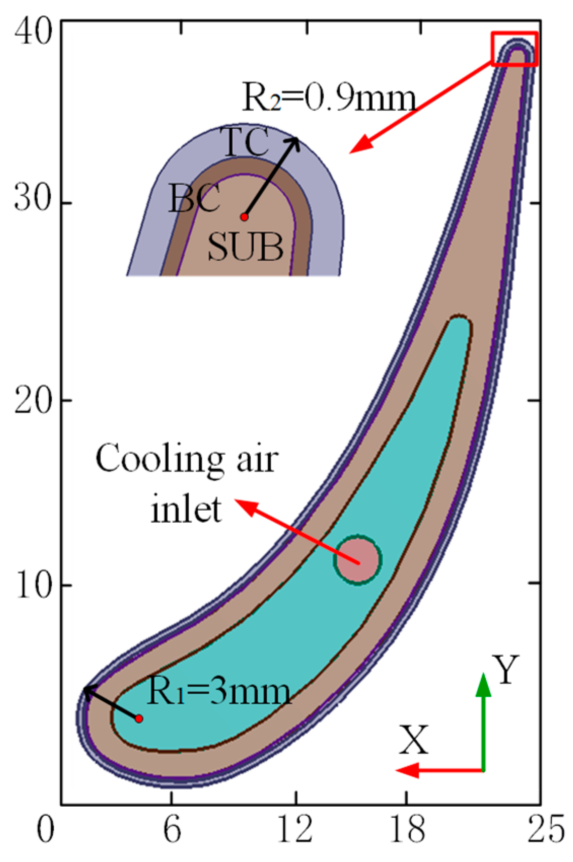
TBC life is seriously induced by four components as shown in Figure 1 [5]: (i) Top coat (TC) layer: providing thermal insulation; (ii) Thermally grown oxide (TGO) layer: providing the bonding of TBC with bond coat (BC) to slow subsequent oxidation; (iii) BC layer: containing the source of elements to create TGO in oxidizing environment and provide oxidation protection; and (iv) superalloy substrate: carrying mechanical loads. Through the oxidation of high-temperature gas, the aluminum in the BC is oxidized to produce an alumina layer (also called the TGO). With the increase in the TGO thickness, the material properties between the TC and BC are destroyed. The mixed layer TC/TGO is liable to crack and peel off under the combined effect of thermal stress and deformation in different layers, which eventually leads to the failure of the NGV [6]. Therefore, it is of some urgency to study the mechanical properties of a mixed layer TC/TGO with regard to a thermal shock environment. Robert [7] presented a Thermo-Calc/Dictra-based approach for the life prediction of isothermally oxidized atmospheric plasma sprayed TBCs. The beta-phase depletion of the coating was predicted and compared to the life prediction criteria based on the TGO thickness and aluminum content in the coating. Based on the BC test results, the life of the TBC was predicted by Song [8], according to degradation and thermal fatigue. Many experiments indicated that the failure of the TBC systems under thermomechanical loading was complicated due to the influences of many factors such as thermal mismatch, oxidation, interface roughness, creep, sintering, and so forth [9,10,11].

Among the failure factors, the effect of TGO growth is particularly prominent, because volume expansion and compressive stress increase are correlative with the growth of TGO. When the NGV gets to the cooling state, the induced unbalanced temperature at the mixed layer TC/TGO leads to a high residual compressive stress, which varies directly with the strain energy. When the strain energy reaches the limit value, cracks occur. Yang et al. [12,13] tested an oxidation weight gain of the TBC at 1323 K and obtained the dynamic test curves for characterizing the TGO thickness. Based on this work, Wei et al. [14] established a TFL model of a TBC regarding the phenomenological approach and low cycle fatigue theory. However, the working environment and micro-strain characteristics of the NGV were not discussed in detail. In the process of the thermal shock cycle, the flow, heat transfer, and structure interact with each other, thus it is difficult to separate the temperature field from thermal stress in the calculation of flow characteristics. Therefore, the TFL of a NGV is a typical fluid-thermo-structure (FTS) coupling problem.

With the development of numerical simulation approaches, it is possible to calculate the thermal shock cyclic loads of a NGV by combining computational fluid dynamics (CFD) and finite element (FE) methods. Kim et al. [15] studied the heat transfer coefficients and stresses on blade surfaces using the finite volume (FV) and FE methods and obtained the maximum material temperature and thermal stress at the trailing edge near mid-span. Meanwhile, he also discussed the life prediction methods of turbine components by coupling aero-thermal simulation with a nonlinear thermal-structural FE model and a slip-based constitutive model [16]. Chung et al. [17] predicted the cracks on the vane of a power generation gas turbine by the FTS method and Guan et al. [18] carried out a simulation investigation of temperature variation, and obtained the stress and vibration characteristics of a NGV by the FTS method.

Although the FTS technology can reveal the physical characteristics of a NGV in the thermal cycle under macroscopic scales, the thermal fatigue problems of TBC gradually emerge from micro-cracks [19]. Up to now, it is possible to establish a mathematical grid model with respect to both the macro and micro scales. However, the solution of the grid model requires huge computing resources and time consumption, which seriously restricts the development of new thermal barrier coated NGVs [20]. Therefore, to provide an effective TFL model of the TBC, it is necessary to integrate flow, heat transfer, and structure with the micro- and macro-scale to perform an integrity design. The concept of high-integrity was proposed by the United States Air Force in 2012 for the numerical simulation of a NGV with a TBC [21]. High-integrity requires the consistency of the numerical simulation with a real structure. Due to the costly computation, however, we have not found related works to highly-integrated TBC simulation so far.

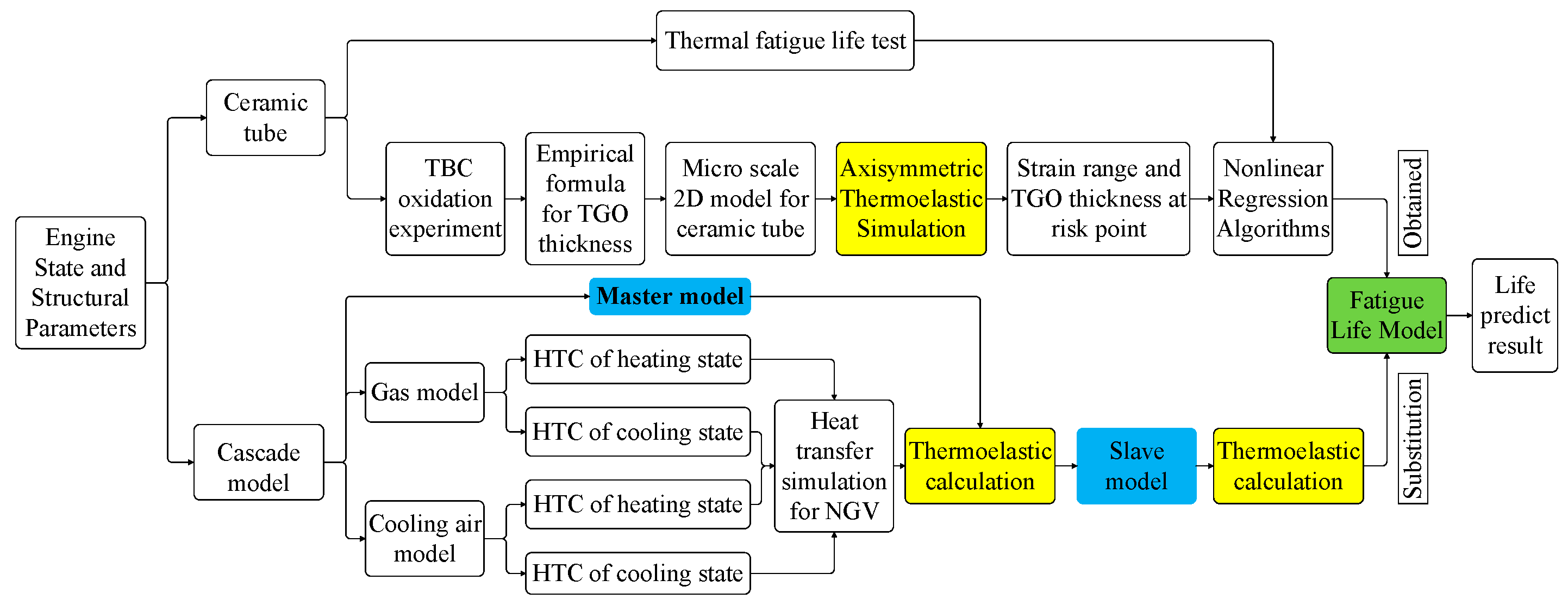
Along with the heuristic thought, it is unsatisfactory for a highly-integrated analysis of the life prediction of a NGV with a TBC to only consider heat shock performance in the macro- or micro-scale. This paper attempts to develop a high-integrity approach, in other words, the master–slave model involving the FTS coupling technology, phenomenological life prediction method, and volume mesh mapping algorithm for TBC thermal fatigue life prediction and the improvement in prediction precision and efficiency. Here, the master–slave model was used to establish the relationship between the macro-scale and micro-scale in the thermal fatigue life prediction of a TBC.

The remainder of this paper is organized as follows. Section 2 introduces the modeling and simulation approaches including the physical model, material parameters, boundary conditions, meshing, and simulation procedure. The verification strategy and establishment of thermal fatigue life are discussed in Section 3. In Section 4, the results and discussion involving the heat transfer analysis, temperature filed analysis, thermo-structural analysis, and thermal fatigue life prediction of the TBC on a NGV are investigated. Section 5 gives the conclusions and findings of this paper.

2. Modeling and Simulation Methods

2.1. Thermal Fatigue Life Theory of Thermal Barrier Coat

To establish the TFL prediction model of the TBC, the classical phenomenological life prediction method proposed by Meier et al. [22] was referred to in this paper. According to the theory, the TFL of the TBC is related to the TGO thickness and strain range in the thermal cycle. The experimental correlation of the TGO layer thickness is described as:

$$\delta ={\left\{\exp \left[Q\left(\frac{1}{T_0}-\frac{1}{T}\right)\right]\cdot t\right\}}^n$$

(1)

where δ, t, and T indicate the TGO thickness, oxidation time, and oxidation temperature, respectively; Q, T₀, and n are the active energy of oxygen atom diffusion in metals, undetermined temperature, and undetermined coefficient, which are 28,230, 1572, and 0.313 at 1320 K, respectively, as determined by the experimental investigation of a plasma sprayed TBC material [13].

The phenomenological TFL model is

$$N={\left[\left(\frac{\mathsf{\Delta }{\epsilon }_{f_o}}{\mathsf{\Delta }{\gamma }_i}+a\mathsf{\Delta }{\epsilon }_i\right)\left(1-\frac{\delta }{{\delta }_c}\right)+\left(\frac{\delta }{{\delta }_c}\right)\right]}^b$$

(2)

where N indicates the number of cycles; Δγ_i and Δε_i are the shear strain range and axial strain range at risk point in the ith thermal cycle, respectively; $\mathsf{\Delta }{\epsilon }_{f_0}$ is the critical tensile strain range; δ_c is the critical TGO thickness; and a and b are unknown parameters in Equation (2).

Regarding $\mathsf{\Delta }{\epsilon }_{f_0}$ = 0.087 and δ_c = 0.058 mm for the plasma sprayed TBC material [14], Equation (2) is considered as a time-dependent oxidation-induced cracking process accompanied by oxidation failure at the mixed TC/TGO layer with respect to the peel off process of the TBC. Miner’s linear cumulative damage model [22] was used to compute cyclic life in this paper.

In cumulative theory, the damage caused by one cycle is assumed to be D_m = 1/N_m. The total damage D caused by multiple cycles is

$$D={\displaystyle \sum _{m=1}^k{D}_m}={\displaystyle \sum _{m=1}^k\frac{1}{N_m}}$$

(3)

where m denotes the number of cycles; N_m is the life under m cycles; and k indicates the maximum number of cycles. When the damage D is larger than 1, the TBC is considered to have failed.

2.2. Simulation Procedure

The high-integrity life prediction approach for the TBC on a NGV with the master–slave model is shown in Figure 2.

To find the coefficients (a and b) in Equation (2), we need the TFL test data of the NGV. Due to the insufficient TFL measurement data of the NGV in an open database [23], the TFL of a typical ceramic metal tube, a similar plasma sprayed TBC material, and the working environment of the model described in this paper, was selected to calculate the value of parameters a and b in Equation (2). The ceramic tube test has been proven to be an effective alternative test method [13]. The prediction procedure of the TFL for the TBC is described as follows:

Step 1: Based on the geometry parameters and test conditions of a ceramic metal tube, a 2D axisymmetric FE model was established and solved by the thermo-elastic method. Both shear strain ranges and axial strain ranges (i.e., strain ranges in the Z direction) at the risk point in one cycle were simulated with different TGO thicknesses, and the relationship of the strain and thickness was obtained by fitting polynomials. The relationship was inputted into Equation (2). According to the cyclic life test of the ceramic metal tube, the parameters a and b were obtained by nonlinear regression analysis.

Step 2: The typical thermal shock test of the NGV was divided into two states (i.e., heating stage and cooling stage). The convection heat transfer coefficient of each stage was solved by the CFD method, and then imported into the master model (i.e., macro NGV with TBC) as the boundary conditions. Then, the temperature and node deformations were solved by the thermo-elastic coupling method. The results at each time were inputted into the slave model (i.e., micro TBC) by the volume element intersection mapping algorithm [24]. The master–slave model was based on two assumptions: (a) The TGO hardly affects the temperature field in the TBC, and (b) the grid node deformation mainly depends on the temperature field at the macro scale [25].

Step 3: The strain ranges at the risk points of the slave model were imported into the TFL model to predict the cyclic life of TBC.

2.3. Physical Model and Meshing Method

The focus of this paper was on the first stage NGV of an axial flow turbojet engine [26]. The flow cascade was comprised of 24 vanes. The internal and external radii of the link rings were 95 mm and 135 mm, respectively. In this study, the fan-shaped cascade was simplified to the square cascade with a vane space of 38 mm, while both cooling holes and link rings were ignored. The geometrical size of the NGV is shown in Figure 3. As illustrated in Figure 3, the geometry of the master model consisted of three layers (i.e., TC (material mode no. 8YSZ with thickness 0.25 mm), BC (material mode no. NiCrAlY with thickness 0.125 mm), and Ni-based alloy substrate (material mode no. GH3030)). The TGO layer only existed in the slave model to calculate the strain range for different thicknesses. The master–slave model is shown in Figure 4a.

Based on the morphological characteristics of the TGO layer [27], a sinusoidal interface, as indicated in Figure 4b, was adopted to approximate the TGO and mixed layer with the wavelength of 0.04 mm and amplitude of 0.01 mm. Three kinds of slave models were established, as seen in Figure 4b, for the TBC with a flat surface, TBC with a sinusoidal interface, and TBC with a TGO layer. As high-temperature regions are usually at the center of the leading edge and trailing edge, two pieces of the TBC layer were defined as the subdomain of the master model in the positions. To prevent a large volume ratio of grid elements in the master model, the subdomain was slightly larger than the slave model.

According to the structure of the master model, the gas and cooling air models were meshed. The thickness of the first layer near the wall grids was 1 μm and the expansion ratio was 1:2. The grids of gas, cooling air, and master model were selected by mesh independence tests with respect to the sizes of the cell of 520,000, 40,000, and 330,000, respectively, and the grid numbers of the subdomain and slave model were 10,000 and 580,000, respectively. All grid models are shown in Figure 4. A fully coupling element, ANSYS-Solid 226 (Provided by workbench 18.0 software, ANSYS, Pittsburgh, PA, USA), was adopted in the master model. The fully coupling technology can improve the accuracy of thermo-elastic coupling by 2% to 3% with regard to temperature displacement coupling theory [28]. As the temperature was already solved in the master model, a weak coupling element, ANSYS-Solid 186, was adopted in the slave model. As for the master–slave model, it is unnecessary to repeatedly build and simulate the FE model with the increase in the TGO thickness. Thus, it is necessary to improve the work efficiency of the TFL prediction.

2.4. Material Parameters and Boundary Conditions

In the above FE model, each layer of the NGV and TBC is considered as an isotropic and homogeneous material. The TC is modeled as an elastic body, whereas the BC, TGO, and substrate are regarded as elastic–perfectly plastic materials [29,30]. The temperature-dependent material properties are listed in

Table 1. Temperature dependent material parameters for different layers [30].

Parameters	SUB	BC	TGO	TC
Temperature, K	20–1100	20–1100	20–1100	20–1100
Thermal expansion coefficient, 10−5/K	1.48–1.80	1.36–1.76	0.80–0.96	0.90–1.22
Young modulus E, GPa	220–120	200–110	400–320	48–22
Poisson ratio v	0.31–0.35	0.30–0.33	0.23–0.25	0.10–0.12
Shear modulus, ×1011 Pa	0.84–0.44	0.77–0.41	1.66–1.28	0.21–0.01
Heat transfer coefficient, W/m·K	88–69	5.8–17	10–4.1	2–1.7
Density, kg/m3	8500	7380	3984	3610
Specific heat, J/kg K	440	450	755	505

and

Table 2. The variations of yield strength with temperature for different layers [31].

No.	Temperature	SUB	BC	TGO
1	300 K	800 MPa	426 MPa	10,000 MPa
2	473 K	800 MPa	412 MPa	10,000 MPa
3	673 K	800 MPa	396 MPa	10,000 MPa
4	873 K	800 MPa	362 MPa	10,000 MPa
5	1073 K	800 MPa	284 MPa	10,000 MPa
6	1273 K	800 MPa	202 MPa	1000 MPa
7	1373 K	800 MPa	114 MPa	1000 MPa

. It should be noted that to limit stress to the experimental level [31,32], the TGO is allowed to undergo stress relaxation at high temperatures, which is realized by introducing the yield strength of TGO at peak temperatures [31]. The multilinear kinematic hardening model was selected to simulate the elastic–plastic behaviors. The back-stress tensor for multilinear kinematic hardening evolves such that the effective stress versus effective strain curve is multilinear with linear segments defined by the stress–strain–temperature points [33]. The yield stress σ_yi (i = 1, 2, …, 7) for the ith temperature point in Table 2 is

$${\sigma }_{yi}=\frac{1}{2\left(1+\nu \right)}\left(3E{\epsilon }_i-\left(1-2\nu \right){\sigma }_i\right)$$

(4)

where (ε_i, σ_i) is stress and strain at the ith temperature point, respectively; E is the Young modulus; and v is the Poisson ratio.

Table 3. Engine performance parameters [26].

Parameters	Value
Inlet average total temperature T*eng, K	290.29 K
Exhaust nozzle total temperature T*ex, K	917.33 K
Inlet static pressure Peng, KPa	95.22 KPa
Compressor outlet total pressure P*com, KPa	538.39 KPa
Inlet air flow of the engine Weng, g/s	3520 g/s
Fuel mass flow Wfu, g/s	54.48 g/s
Mach number of engine inlet Maeng	0.31

reveals the performance parameters of the axial flow turbojet engine, which are employed to derive the simulated boundary conditions of the master model.

In line with the power balance principle of the aeroengine rotor shaft, the relationship between the inlet Mach number Ma_eng and the engine inlet total pressure P^*_eng is

$$P_{\mathrm{eng}}^{*}=P_{\mathrm{eng}}{\left(1+0.2\cdot M{a}_{\mathrm{eng}}{}^2\right)}^{3.5}$$

(5)

where P_eng is the inlet static pressure.

With respect to the efficiency of compressor η_com = 0.89 [34], the outlet temperature of compressor T^*_com is

$$T_{\mathrm{com}}^{*}=T_{\mathrm{eng}}^{*}\left(1+\frac{{\pi }^{0.2857}-1}{{\eta }_{\mathrm{com}}}\right)$$

(6)

where π = P^*_com/P^*_eng is the pressure ratio of the compressor and T^*_eng is the total temperature of engine inlet.

The temperature of the cooling air is determined by the outlet temperature of the compressor because cooling air is sucked up directly from the end of compressor. In light of Equations (4)–(6), the cooling air mass flow W_c, mean temperature T_mean at the cascade inlet, and inlet total pressure P_in^* are computed by

$$W_{\mathrm{c}}=W_{\mathrm{eng}}\left[\left(1-w\right)\left(1+F\right)+w\right]$$

(7)

$$T_{\mathrm{mean}}=\frac{C_{\mathrm{g}}{W}_{\mathrm{eng}}{T}_{\mathrm{com}}^{*}}{C_{\mathrm{pg}}{W}_{\mathrm{c}}{\eta }_{\mathrm{sh}}}+T_{\mathrm{ex}}^{*}$$

(8)

$$P_{\mathrm{in}}^{*}=P_{\mathrm{com}}^{*}\cdot {\eta }_{\mathrm{rs}}$$

(9)

where w = 1.88% is the percentage of coolant flow; F = W_fu/W_eng is the gas–oil ratio, where W_fu is the oil mass and W_eng is the gas mass flow; C_g is the specific heat capacity of air; C_pg is the specific heat capacity of hot gas; η_sh = 99% is the mechanical efficiency of aeroengine shaft; η_rs = 0.97 is the total pressure recovery coefficient of combustor [34]; T*_ex indicates exhaust temperature; and P*_com expresses the inlet total pressure of compressor.

In terms of Equations (5)–(9), the conditions of the NGV simulation are shown in

Table 4. Simulation conditions of the NGV.

Variable	Value
Inlet total pressure, Pin*	522 KPa
Inlet average temperature, Tmean	1310 K
Outlet mass flow, Wout	148.9 g/s
Cooling air mass flow, Wca	2.8 g/s
Cooling air inlet total temperature, T*com	491 K

.

All boundaries were set as no-slip walls, and the periodic boundary method was used to predict periodic flow. The influence of gas kinetic energy on heat transfer is considered by the total energy model. The selected turbulence model SST γ-θ, which is usually used in the simulation of cascades, has a high prediction accuracy [35]. The solution scheme of the model is the second-order backward Euler method [36]. When the residue error of mass flow is less than 10⁻⁶, the calculation is considered to be convergent. The bottom surface of the NGV was restrained in the z direction and the top surface was constrained in the x and y directions.

3. Life Modeling Process

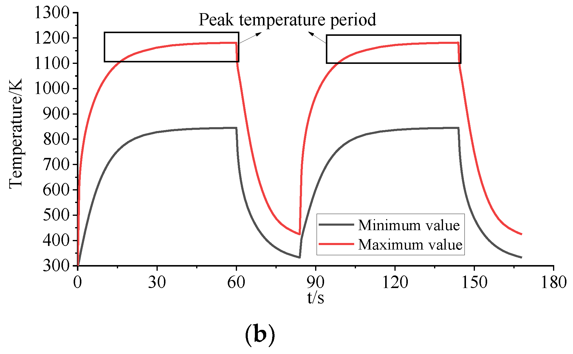
The TFL test data of the ceramic metal tube were adopted to build the phenomenological TFL model (Equation (2)) by finding parameters a and b. The inner diameter, outer diameter, and length of the ceramic metal tube were 11 mm, 15 mm, and 85 mm, respectively. In the TFL test experiment, the central region of the tube with the length of 50 mm was heated for 160 s by an electromagnetic induction coil. After heating, the inner surface was cooled for 260 s by high pressure air [13]. The measured interface temperature of the TBC in a single cycle are shown in Figure 5. The TFL of a typical NGV was tested under six operating conditions (case 1, case 2, …, case 6). The results of the tests are shown in

Table 5. Test results of the thermal fatigue experiment under a preheating temperature of 1323 K [14].

Number	Test Condition		Cycle
	Preheating Time, H	Heat Preservation Time, S
Case 1	0	0	298
Case 2	0	670 s	505
Case 3	50 h	0	480
Case 4	100 h	0	441
Case 5	200 h	0	400
Case 6	300 h	0	206

.

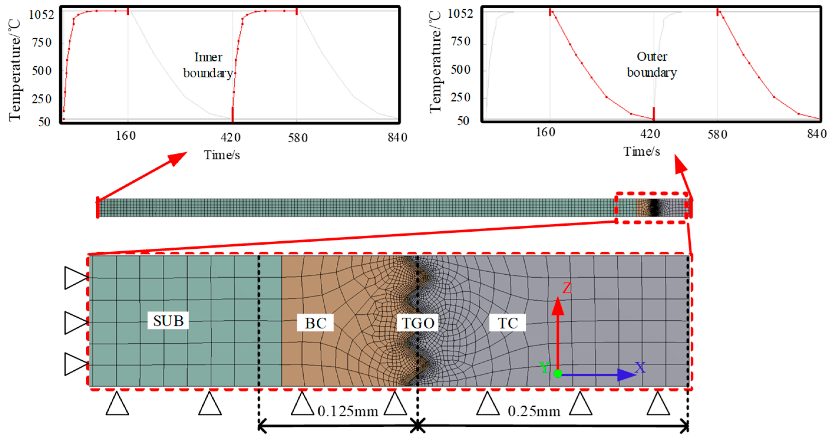
The 2D axisymmetric FE model was established by adopting a micro-segment with the length of 0.125 mm in the center of the heating part, as shown in Figure 6. In the 2D FE model, the size, structure, and material of the TBC layers were consistent with the slave model, and the thermal cyclic load and heating/cooling period were also the same as those in the test. We separated the measured temperature to the cooling temperature curve and heating temperature curve, which were assigned to the inner boundary and outer boundary of the 2D axisymmetric finite element model, respectively. Displacement constraints in the z direction and x direction were applied to the lower edge and inner edge, respectively. A fully coupling element, ANSYS-Plane 223, was used to simulate the transient temperature and thermal stress based on the thermoelastic damping matrix, i.e.,

$$\left[\begin{array}{cc}\left[M\right]& \left[0\right]\\ \left[0\right]& \left[0\right]\end{array}\right]\left\{\begin{array}{c}\left\{\ddot{u}\right\}\\ \left\{\ddot{T}\right\}\end{array}\right\}+\left[\begin{array}{cc}\left[C\right]& \left[0\right]\\ \left[C^{tu}\right]& \left[C^t\right]\end{array}\right]\left\{\begin{array}{c}\left\{\dot{u}\right\}\\ \left\{\dot{T}\right\}\end{array}\right\}+\left[\begin{array}{cc}\left[K\right]& \left[K^{ut}\right]\\ \left[0\right]& \left[K^t\right]\end{array}\right]\left\{\begin{array}{c}\left\{u\right\}\\ \left\{T\right\}\end{array}\right\}=\left\{\begin{array}{c}\left\{F\right\}\\ \left\{Q\right\}\end{array}\right\}$$

(10)

where [M], [C], and [K] are the matric of element mass, element structural damping, and element stiffness, respectively; {u} and {T} are the vector of displacement and temperature, respectively; {F} indicates the um of the element nodal force; [C^t] and [K^t] are the matric of element specific heat, element thermal conductivity, respectively; {Q}, [K^ut], and [C^tu] denote the sum of the element heat generation load and element convection surface heat flow, the matrix of element thermoelastic stiffness, and the matrix of element thermoelastic damping, respectively.

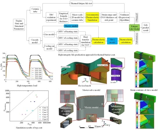
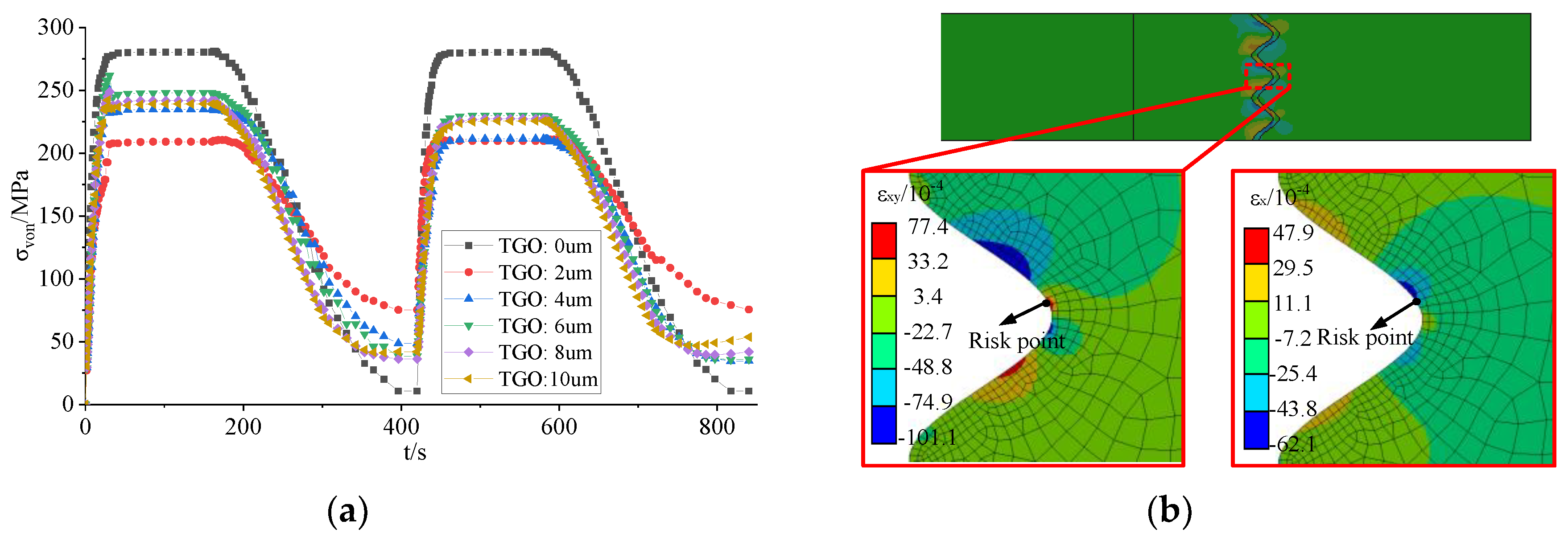
Six typical TGO thicknesses (0, 2 μm, 4 μm, 6 μm, 8 μm, and 10 μm) were selected in the simulation. To find the risk time and point in the thermal cycle, the von-Mises stress was selected, i.e.,

$${\sigma }_{\mathrm{von}}={\left[\frac{{\left({\sigma }_{\mathrm{x}}-{\sigma }_{\mathrm{y}}\right)}^2+{\left({\sigma }_{\mathrm{x}}-{\sigma }_{\mathrm{z}}\right)}^2+{\left({\sigma }_{\mathrm{y}}-{\sigma }_{\mathrm{z}}\right)}^2}{2}\right]}^{\frac{1}{2}}$$

(11)

The maximum thermal stress of the TC layer is shown in Figure 7a. As seen in Figure 7a, the change in thermal stress basically agrees with the temperature curve in Figure 5, and the thermal stress increased with the increasing TGO thickness. The maximum thermal stress occurred in 50 s to 160 s in the first cycle. For the strain contour at the thickness of 2 μm, the shear strain and axial strain are shown in Figure 7b. The results in Figure 7b show that the maximum shear strain and axial strain are near by the bottom of the valley (i.e., point I and II, respectively). The cracks caused by shear strain were perpendicular to the mixed layer of the TGO, while the cracks induced by axial strain were tangent to the valley center (z direction in Figure 6). The value of the shear strain was higher than that of the axial strain, thus the grid node of shear strain was regarded as the risk point for the simulation. The axial and shear strain ranges at the risk point in one thermal shock cycle were imported into Equation (2), and the relationship equations of TBC thickness and strain under the ith operation condition were fitted as

$$\{\begin{array}{l}\mathsf{\Delta }{\gamma }_i=0.00856-4.649\cdot \delta +1613\cdot {\delta }^2-183023\cdot {\delta }^3+7.58\times {10}^6\cdot {\delta }^4\\ \mathsf{\Delta }{\epsilon }_i=0.0058-4.213\cdot \delta +1308\cdot {\delta }^2-160674\cdot {\delta }^3+6.71\times {10}^6\cdot {\delta }^4\end{array}$$

(12)

According to Equation (11), Equation (1) and the cyclic data in Table 5, the coefficients of Equation (2) can be obtained (i.e., a = 54, b = 3.45). In the same condition, more thermal fatigue test data are provided by Geng [37], and applied to verify the accuracy of the TFL model. The verification results are illustrated in Figure 8. As revealed in Figure 8, all of the TFL points were almost distributed in triple dispersion zone, which supports the validity and feasibility of the fitted phenomenological life prediction model.

4. Thermal Cycle Analysis and Life Prediction of NGV.

4.1. Temperature Field Analysis

In general, the temperature curve of the thermal shock test is a series of trapezoidal waves, thus it is difficult to simulate the heat transfer process considering the time-varying momentum and temperature. As the heat transfer rate of gas is much larger than that of metals [18], the heating process of hot gas was neglected in the numerical simulation. With respect to the simulation study, a typical gas cycle profile is shown in Figure 9.

According to the heating cycle, the inlet temperatures of the heating stage and cooling stage were 1310 K and 300 K, respectively. Based on the steady state conjugate heat transfer simulation, the heat transfer boundary conditions were obtained. The convection heat transfer coefficient is:

$$h=\frac{q}{T_{\mathrm{sp}}-T_{\mathrm{aw}}}$$

(13)

where q is the wall heat flux; T_aw is the wall temperature; and T_sp is the mean temperature at the inlet.

Through different combinations of wall temperature and mean temperature as listed in

Table 6. Temperature parameters.

Domain	Fatigue Test Cycle	Taw	Tsp
Hot gas	Heating stage	300 K	1310 K
	Cooling stage	1000 K	300 K
Cooling air	Heating stage	300 K	500 K
	Cooling stage	1000 K	500 K

, the convection heat transfer coefficients of different domains and stages were calculated. The convective heat transfer coefficient of the heating and cooling stages are shown in Figure 10.

As revealed in Figure 10, the high-speed heat transfer regions were located on the leading edge, trailing edge, and the center of the inner surface of the master model, respectively. The convection heat transfer coefficient at the leading edge was larger because the leading edge was directed against the flow direction of the hot gas, and the kinetic energy and internal energy were directly converted to surface temperature. At the trailing edge, the high-temperature gas flowed along the surfaces of both the suction side (SS) and pressure side (PS), then mixed to form a strong turbulence intensity. The increase in the turbulent energy increased the heat transfer rate. In addition, the convective heat transfer coefficient of the heating stage was larger than that of the cooling stage due to the high gas speed in a high-temperature environment.

Based on the acquired convective heat transfer coefficient of the heating and cooling stages, the master model was applied to the thermo-elastic coupling calculation of the NGV for 168 s under the thermal cycle, where the heat fluxes at the upper and lower surface were 10,000 w/m², referring to the solid rim [39]. The variation trend of the surface temperature field is shown in Figure 11.

As shown in Figure 11, the surfaces of the leading edge and trailing edge were heated first, and then reached the maximum temperature quickly. The two areas corresponded to regions A and B in the master model in Figure 4a. In the heat transfer process in Figure 11b, the surface temperature of the NGV rose rapidly toward a stable value after 15 s.

4.2. Temperature Test

To verify the thermal-elastic simulation of the NGV, temperature-sensitive paint (TSP) technology was adopted to measure the surface temperatures of the NGV under the maximum operation conditions of a turbojet engine. The surface temperature tests for the NGV were performed inside an indoor aero-engine test rig at the China Gas Turbine Establishment, the structure of which is shown in Figure 12. The technical parameters of the engine are listed in Table 3.

As each TSP material has one dedicated temperature sensitive range, only temperatures can be recorded in this range in the TSP test. Two typical TSP were selected to show the temperature distributions in the NGV. Isothermal lines (also called discoloration lines) were drawn to calibrate and explain the TSPs instead of the colors after heating. The calibrated temperatures of the thermal-indicate standard models under the constant peak temperature for 180 s are shown in Figure 13. In the coming work, the colors of the TSP-M02 and TSP-M05 were referred to determine the temperature distributions gained in the thermal-elastic simulation of the NGV in Section 4.

For the high-integrity approach with the master–slave model, the accuracy of the TFL depends highly on the prediction precision of the temperature field. According to the simulation, we found that the temperature distribution of the NGV was stable after 60 s, at which the temperature fields were compared with the result of the TSP test as shown in Figure 14.

As revealed in Figure 14, the temperature range of the leading edge and trailing edge were 1021 K to 1126 K and larger than 1070 K, respectively. The maximum temperature of the TSP test was a bit higher than the simulation. The film cooling technology was used to reduce the surface temperature. Therefore, the simulation temperature was reasonable. Compared with traditional methods, the prediction accuracy of the temperature field was improved by using the fully coupled technology in the heat transfer simulation [18]. Furthermore, the temperatures at the center of the leading edge and the trailing edge were 1177 K and 1205 K, respectively, which were similar to that of the ceramic metal tube test and indicate that the parameters in the oxidation weight gain model are also applicable to the NGV.

4.3. Matching of Master Model and Slave Model

To transfer the boundary displacement and body temperature data from the master model (i.e., source) to the slave model (i.e., target), we reasonably adopted the volume element intersection mapping algorithm [24]. The first step in the process of the volume element intersection mapping algorithm is to divide the mapping source mesh into an imaginary structured grid, with each grid section called a “bucket.” Next, each node on the data transfer regions of the target mesh is initially associated with a bucket. For the master–slave model discussed in this paper, the subdomain of master model was large enough to hold the mesh element of slave model as shown in Figure 4a. Therefore, the volume element intersection mapping algorithm was used to match each of the target nodes to one source element in the bucket. This was done by looping through all the source elements in that bucket and checking to see whether the target node was within their domain or not. The transferring results are displayed in Figure 15. Obviously, the imported data in the slave model still retained the distribution of temperature and deformation in the master model, although the mesh number of the master model and slave model was different.

To validate the validity of the volume element intersection mapping algorithm, we performed a high-integrity thermal fatigue life analysis with the transferred slave model without both TGO and sinusoidal interface. The thermal stress comparison on the TC layer of master model and slave model is shown in Figure 16. The results in Figure 16 show that in the same thermal cycle, the stress variations of the slave model agreed well with the master model, because the maximum error was less than 1%. Furthermore, the trailing edge endured a large thermal shock load, especially at the beginning of the heating and cooling stage. Compared to Figure 11, the heat transfer rate at the trailing edge was much larger than that of the leading edge, so that under a high thermal load, a large temperature gradient was produced to induce a high thermal stress level. Therefore, compared with the traditional simulation method, the high-integrity analysis approach is more likely to find out the essential reasons that lead to thermal fatigue failure.

4.4. Thermal Fatigue Life Analysis of Nozzle Guide Vane with TBC

When the TGO thickness was 2 μm, the thermal stress simulation results in the TC layer based on the slave model with sinusoidal interface are as shown in Figure 17. Compared to Figure 16, the thermal stress in Figure 17 changed smoothly on the sinusoidal interface, because the shape of the mixed TC/TGO layer was a buffer. Furthermore, we found that the risk moment was at the beginning of the cooling stage. The strain contours of the slave model at 60.6 s are drawn in Figure 18.

As shown in Figure 18, the peaks of the shear strain and axial strain occurred near the mixed TC/TGO layer, and the maximum strain point was in the valley region. The distributions of the shear and axial strain were basically consistent with those of the ceramic tube in Figure 7b. The reason for this is that the thermal stress level of the mixed TC/TGO layer at the trailing edge was affected by the total deformation of the master model. The leading edge and trailing edge can be considered as a series of ceramic tubes with different radii, which is also the reason for why the distribution of the thermal strain was similar to the slave model and ceramic tube model. The stress and strain at the risk point in the mixed TC/TGO layer were almost independent with the radius of the ceramic tube [14]. As a result, the TFL model of ceramic tubes previously established is also applicable to the high-integrity life prediction of a NGV. The grid node at the shear strain concentration points highlighted in Figure 18 was regarded as the crack initiation point (i.e., risk point) as the shear strain was much higher than the axial strain. The stress–strain curves at the risk point are shown in Figure 19.

As revealed in Figure 19, the integral area (red and black region) and strain range of the stress–strain curve of the trailing edge were larger than that of the leading edge (black region), indicating that the thermal shock attacking at the leading edge has a stronger failure energy under the same thermal cycle. On the other side, the fatigue hysteresis loops at the risk point basically reached a stable state, indicating that the thermal stress of the TC layer reached the plastic stability stage after two thermal cycles (i.e., the axis and shear strain range do not vary by repeating the thermal cycle simulation). Thus, the thermal strain range at the second thermal cycle was inputted into the TFL model.

By repeatedly producing the high-integrity TFL analysis of the NGV, the thermal strain ranges of six TGO thicknesses (i.e., 0, 2 μm, 4 μm, 6 μm, 8 μm, and 10 μm) were obtained as shown in Figure 20.

As shown in Figure 20, the strain levels at the sinusoidal interface regions were correlated with TGO thickness. The axial strain ranges were basically smaller than the shear strain range, and the changing trends of the axial strain ranges at both the leading edge and trailing edge were opposite the shear strain ranges. The strain ranges of the TC layer did not change much at the beginning of the thermal cycles, but the shear strain ranged increased obviously with the increase in the TGO thickness, which indicates that shear strain is a key factor inducing the thermal fatigue of the TBC material. The varying trends of strain range at the leading and trailing edge were similar, proving that the corner radius slightly influences the micro-strain. The fitted equations of the TGO thickness and strain range at the risk points are as follows.

Strain range of leading edge:

$$\{\begin{array}{l}\mathsf{\Delta }{\gamma }_i=0.00369+1.139\cdot \delta +172\cdot {\delta }^2-49908\cdot {\delta }^3+2.91\times {10}^6\cdot {\delta }^4\\ \mathsf{\Delta }{\epsilon }_i=0.00364-1.508\cdot \delta +283\cdot {\delta }^2-1933\cdot {\delta }^3+3.49\times {10}^5\cdot {\delta }^4\end{array}$$

(14)

Strain range of trailing edge:

$$\{\begin{array}{l}\mathsf{\Delta }{\gamma }_i=0.0025+2.64\cdot \delta -380\cdot {\delta }^2+38204\cdot {\delta }^3-1.69\times {10}^6\cdot {\delta }^4\\ \mathsf{\Delta }{\epsilon }_i=0.00198+2.1\cdot \delta -753\cdot {\delta }^2+84741\cdot {\delta }^3-3.04\times {10}^6\cdot {\delta }^4\end{array}$$

(15)

Importing Equations (13) and (14) into the TFL model, the cumulative damage is calculated to gain the number of the TBC cyclic life as shown in

Table 7. Thermal fatigue life of the TBC on the NGV.

Number	Life Cycle		Thermal Fatigue Life
	Leading Edge, N	Trailing Edge, N	Leading Edge, H	Trailing Edge, H
Case 1	1892	1558	40	33
Case 2	1345	870	279	180
Case 3	1419	916	30	20
Case 4	1310	704	28	15
Case 5	1126	558	24	12
Case 6	895	536	19	11

.

As demonstrated in Table 7, the service life of the NGV was reduced with the increase in the TGO thickness. The thermal life of the TBC at the trailing edge was shorter than that at the leading edge. Darolia [5] found that the peel off life cycle of the TBC on a NGV with a NiAl composition at 1448 K was about 1500 times. The thermal cyclic test in [40] clarified that 5–10% spallation of the BC layer happened during 1500–2000 cycles under the temperature of 1323 K. Therefore, the developed master–slave model was validated to be sufficiently accurate for the high-integrity life prediction.

5. Conclusions

The target of this paper was to propose an efficient master–slave model for the thermal fatigue life (TFL) prediction method of a nozzle guide vane (NGV) with a thermal barrier coat (TBC), with respect to flow-thermo-structural coupling, oxidation damage, and thermal fatigue damage. The modeling and simulation methods and life molding processes were first investigated and validated. Then, the TFL prediction method of the NGV with the TBC was performed with respect to the proposed master–slave model in the foundation of the temperature filed analysis, temperature test, and matching of the master and slave models. Through these studies, some conclusions and findings can be summarized as follows:

(1) The adopted SST γ-θ turbulence model effectively predicted the convective heat transfer coefficient by thermal-elastic simulation, and the temperature field solved by the fully coupled solid 226 element agreed well with the test data of the aircraft engine. This revealed that the fully coupling solid 226 element is promising to improve the accuracy of the temperature field calculation. Compared with the traditional method, the accuracy of the temperature field calculation was improved by over 5%.

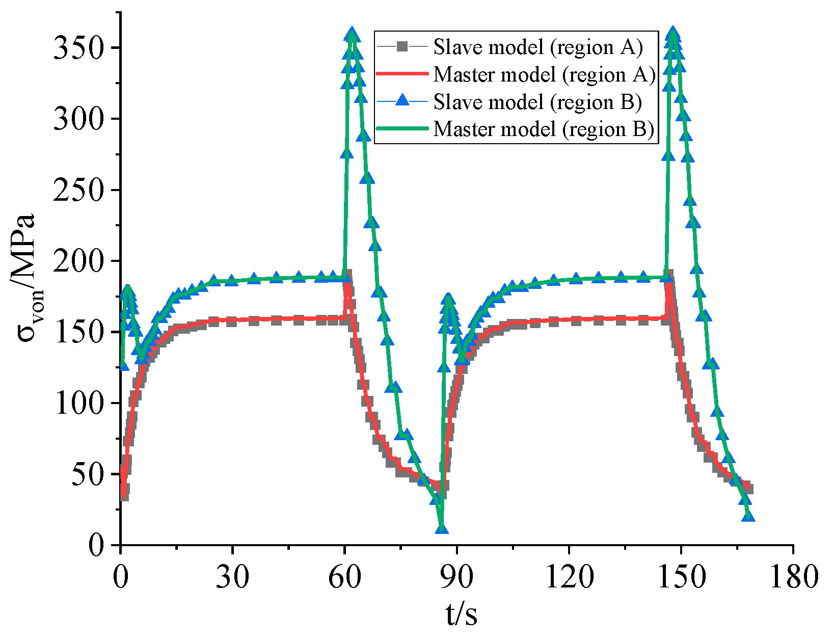
(2) Based on the volume element intersection mapping algorithm, the boundary conditions of the temperature and displacement were successfully transferred from the master model into the slave model with high precision. The simulation results of the master model and slave model showed good agreement, indicating that it is possible to link macro- and micro-scales with the master–slave model presented in this paper.

(3) The ranges of the axial and shear strains in the TC layer were affected by the thickness of the TGO layer, but the trends of the two kind strains were almost the opposite. With the increase in the thermal cyclic number, shear strain plays a dominant role in the life model because it seriously effects the TFL prediction of the TBC on a NGV for an aero engine.

(4) Based on the developed master–slave model, the TFL of a typical NGV was precisely predicted with minor errors when compared to the test data, and the life variation also met the actual usage of the NGV. The proposed method comprehensively considers the physical characteristics of heat transfer boundaries, macro-scale and micro-scale to reflect the coupling failure of oxidation damage and thermal fatigue.

In short, the developed master–slave model was validated to be highly-computationally precise and efficient with regard to TFL prediction for a NGV with a TBC by comparing the temperature and the life cycle of the key points at the leading edge and trailing edge with the experiments. The efforts of the study provide a promising modeling strategy (master–slave model) for the integrated TFL prediction design of thermal structures other than NGV in engineering.

References

1. Ebrahimi, H.; Nakhodchi, S. Thermal fatigue testing and simulation of an APS TBC system in presence of a constant bending load. Int. J. Fatigue 2017, 96, 1–9. [Google Scholar] [CrossRef]
2. Zhang, C.Y.; Wei, J.S.; Jing, H.Z.; Fei, C.W.; Tang, W.Z. Reliability-Based Low Fatigue Life Analysis of Turbine Blisk with Generalized Regression Extreme Neural Network Method. Materials 2019, 12, 1545. [Google Scholar] [CrossRef] [PubMed]
3. Zhang, C.Y.; Yuan, Z.S.; Wang, Z.; Fei, C.W.; Lu, C. Probabilistic Fatigue/Creep Optimization of Turbine Bladed Disk with Fuzzy Multi-Extremum Response Surface Method. Materials 2019, 12, 3367. [Google Scholar] [Green Version]
4. Sheffler, K.D.; Gupta, D.K. Current status and future trends in turbine application of thermal barrier. ASME J. Eng. Gas Turbine Power 1988, 110, 605–609. [Google Scholar] [CrossRef]
5. Darolia, R. Thermal barrier coatings technology: Critical review, progress update, remaining challenges and prospects. Int. Mater. Rev. 2013, 58, 315–348. [Google Scholar] [CrossRef]
6. Ranjbar-Far, M.; Absi, J.; Mariaux, G.; Dubois, F. Simulation of the effect of material properties and interface roughness on the stress distribution in thermal barrier coatings using finite element method. Mater. Des. 2010, 31, 772–781. [Google Scholar] [CrossRef]
7. Robert, E.; Kang, Y.; Sten, J.; Ru, L.P. Microstructure-Based Life Prediction of Thermal Barrier Coatings. Key Eng. Mater. 2013, 592–593, 413–416. [Google Scholar]
8. Song, H.; Lee, J.M.; Kim, Y.; Oh, C.S. Evaluation of Effect on Thermal Fatigue Life Considering TGO Growth. J. Korean Soc. Prec. Eng. 2014, 31, 1155–1159. [Google Scholar] [CrossRef]
9. Guan, P.; Ai, Y.T.; Fei, C.W. An enhanced flow-thermo-structural modeling and validation for the integrated analysis of film cooling nozzle guide vane. Energies 2019, 12, 2775. [Google Scholar] [CrossRef]
10. Xie, W.G.; Eric, J.; Maurice, G. Stress and cracking behavior of plasma sprayed thermal barrier coatings using an advanced constitutive model. Mater. Sci. Eng. A 2006, 419, 50–58. [Google Scholar] [CrossRef]
11. Song, L.K.; Bai, G.C.; Fei, C.W.; Tang, W.Z. Multi-failure probabilistic design for turbine bladed disks using neural network regression with distributed collaborative strategy. Aerosp. Sci. Technol. 2019, 92, 464–477. [Google Scholar] [CrossRef]
12. Yang, X.G.; Geng, Y.; Zhou, H.P. An Experimental Study of Oxidation and Thermal Fatigue of TBC. J. Aerosp. Power 2003, 18, 195–200. [Google Scholar]
13. Yang, X.G.; Geng, Y.; Zhou, H.P. A Study of Thermal Fatigue Life Prediction of TBC. J. Aerosp. Power 2003, 18, 201–205. [Google Scholar]
14. Wei, H.L.; Yang, X.G.; Qi, H.Y. Study on thermal fatigue life prediction for plasma sprayed thermal barrier coatings on the surface of turbine vane. J. Aerosp. Power 2008, 23, 1–8. [Google Scholar]
15. Kim, K.M.; Park, J.S.; Dong, H.L.; Lee, T.W.; Cho, H.H. Analysis of conjugated heat transfer, stress and failure in a gas turbine blade with circular cooling passages. Eng. Fail. Anal. 2011, 18, 1212–1222. [Google Scholar] [CrossRef]
16. Kim, K.M.; Yun, H.J.; Yun, N.; Dong, H.L.; Cho, H.H. Thermo-mechanical life prediction for material lifetime improvement of an internal cooling system in a combustion liner. Energy 2011, 36, 942–949. [Google Scholar] [CrossRef]
17. Chung, H.; Sohn, H.S.; Park, J.S.; Kim, K.M.; Cho, H.H. Thermo-structural analysis of cracks on gas turbine vane segment having multiple airfoils. Energy 2017, 118, 1275–1285. [Google Scholar] [CrossRef]
18. Guan, P.; Ai, Y.T.; Wang, Z.; Wang, F. Numerical Simulation of Nozzle Guide Vane Subjected to Thermal Shock Load. J. Propuls. Technol. 2016, 37, 1938–1945. [Google Scholar]
19. Zhu, W.; Wang, J.W.; Yanga, L.; Zhoua, Y.C.; Wei, Y.G.; Wu, R.T. Modeling and simulation of the temperature and stress fields in a 3D turbine blade coated with thermal barrier coatings. Surf. Coat. Technol. 2017, 315, 443–453. [Google Scholar] [CrossRef]
20. Staroselsky, A.; Martin, T.J.; Cassenti, B. Transient thermal analysis and viscoplastic damage model for life prediction of turbine components. J. Eng. Gas Turbines Power 2015, 137, 042501. [Google Scholar] [CrossRef]
21. Johnson, J.J.; King, P.I.; Clark, J.P.; Koch, P.J. Exploring conjugate CFD heat transfer characteristics for a film-cooled flat plate and 3-D turbine inlet vane. In Proceedings of the ASME Turbo Expo, Copenhagen, Denmark, 11–15 June 2012. [Google Scholar]
22. Meier, S.M.; Nissley, D.M.; Sheffler, K.D. Thermal Barrier Coating Life Prediction Model Development, Phase II Final Report; NASA-CR-189111; Pratt and Whitney Aircraft: East Hartford, CT, USA, 1991. [Google Scholar]
23. China Aviation Materials Manual Commission. China Aeronautical Materials Handbook; Standards Press of China: Beijing, China, 2002; Volume 9, pp. 117–128. [Google Scholar]
24. Barnett, R.M.; Murphy, M.; Deutsch, C.V. A grid mapping algorithm for modeling with geometric transforms. Comp. Geosci. 2019, 126, 9–20. [Google Scholar] [CrossRef]
25. Nowinski, J.L. Theory of Thermoelasticity with Applications; Martinus Nijhoff Publishers: Hague, The Netherlands, 1978. [Google Scholar]
26. Xiong, Q.R.; Shi, X.J.; Xu, F.; Zhong, M. Surface temperature measurement of turbine nozzle based on temperature-sensitive paint. Gas Turbine Exp. Res. 2014, 27, 45–48. [Google Scholar]
27. Zhu, W.; Cai, M.; Yanga, L.; Guod, J.W.; Zhoua, Y.C.; Lue, C. The effect of morphology of thermally grown oxide on the stress field in a turbine blade with thermal barrier coatings. Surf. Coat. Technol. 2015, 276, 160–167. [Google Scholar] [CrossRef]
28. Bao, T.N. Numerical Study on Thermal Shock of Turbine Guide Vane Considering Thermoelasticity Coupling Effect. Ph.D. Thesis, Shenyang Aerospace University, Shenyang, China, 2018; pp. 18–26. [Google Scholar]
29. Kim, G.M.; Yanar, N.M.; Hewitt, E.N.; Pettit, F.S.; Meier, G.H. The effect of the type of thermal exposure on the durability of thermal barrier coatings. Scr. Mater. 2002, 46, 489–495. [Google Scholar] [CrossRef]
30. Rösler, J.; Bäker, M.; Aufzug, K. A parametric study of the stress state of thermal barrier coatings: Part I: Creep relaxation. Acta Mater. 2004, 52, 4809–4817. [Google Scholar]
31. Veal, B.W.; Paulikas, A.P.; Hou, P.Y. Tensile stress and creep in thermally grown oxide. Nat. Mater. 2006, 5, 349–351. [Google Scholar] [CrossRef]
32. Wang, X.; Xiao, P. Residual stresses and constrained sintering of YSZ/Al2O3 composite coatings. Acta Mater. 2004, 52, 2591–2603. [Google Scholar] [CrossRef]
33. Fei, C.W.; Lu, C.; Liem, P.R. Decomposed-coordinated surrogate modeling strategy for compound function approximation in a turbine-blisk reliability evaluation. Aerosp. Sci. Technol. 2019, 105466. [Google Scholar] [CrossRef]
34. Lian, X.C.; Wu, H. Principles of Aeroengine; Northwest Polytechnic University Press: Xi’an, China, 2005; pp. 152–161. [Google Scholar]
35. Wang, Z.; Wang, D.; Liu, Z.; Feng, Z. Numerical analysis on effects of inlet pressure and temperature non-uniformities on aero-thermal performance of a HP turbine. Int. J. Heat Mass Transf. 2017, 104, 83–97. [Google Scholar] [CrossRef]
36. Wang, Z.D.; Liu, Z.F.; Feng, Z.P. Influence of mainstream turbulence intensity on heat transfer characteristics of a high pressure turbine stage with inlet hot streak. ASME J. Turbomach. 2015, 138, 041005. [Google Scholar] [CrossRef]
37. Geng, D. Strength Analysis and Life Prediction Study on Thermal Barrier Coatings. Ph.D. Thesis, Beijing University of Aeronautics and Astronautics, Beijing, China, 1990. [Google Scholar]
38. Peng, Z.Y.; Lu, W.L. A comparative test approach for thermal fatigue life of high-heat blade under thermal shock. J. Aerosp. Power 1997, 12, 33–36. [Google Scholar]
39. Guan, P.; Ai, Y.T.; Wang, Z.; Bao, T.N. Structure strength simulation of film cooling vane after heat shock by thermal/flow/structure coupling. J. Aerosp. Power 2018, 33, 1811–1820. [Google Scholar]
40. Jonnalagadda, K.P.; Eriksson, R.; Lib, X.H.; Peng, R.L. Thermal barrier coatings: Life model development and validation. Surf. Coat. Technol. 2019, 362, 293–301. [Google Scholar] [CrossRef]
Figure 1. Thermal barrier coating and its four components. TC: Top coat; TGO: Thermally grown oxide.
Applsci 09 04357 g001
Figure 2. High-integrity life predication approach for the thermal barrier coat (TBC) on NGV.
Applsci 09 04357 g002
Figure 3. Section view (mm).
Applsci 09 04357 g003
Figure 4. Meshing of the NGV and master–slave models. (a) Master–slave model; (b) Typical slave models; (c) Flow domain.
Applsci 09 04357 g004
Figure 5. Interface temperature of the TBC in a single cycle [13].
Applsci 09 04357 g005
Figure 6. Finite element (FE) model and boundary conditions of the ceramic metal tube.
Applsci 09 04357 g006
Figure 7. Simulation results of the top coat (TC) layer in ceramic metal tube. (a) Maximum von-Mises stress in TC layer; (b) Strain contour of 2 μm.
Applsci 09 04357 g007
Figure 8. Thermal fatigue test and simulated data [14,37].
Applsci 09 04357 g008
Figure 9. Typical gas cycle profile of the thermal fatigue test [38].
Applsci 09 04357 g009
Figure 10. Convection heat transfer coefficient of the heating and cooling stages. (a) Heating stage; (b) Cooling stage.
Applsci 09 04357 g010
Figure 11. Variation trend and temperature curves with heating time. (a) Change of temperature contour with heating time; (b) Changing curves of maximum and minimum temperature.
Applsci 09 04357 g011aApplsci 09 04357 g011b
Figure 12. Indoor aeroengine test rig [26].
Applsci 09 04357 g012
Figure 13. Temperature test of the standard temperature-sensitive paint (TSP) model.
Applsci 09 04357 g013
Figure 14. Comparison of the predicted temperature contour with the TSP test.
Applsci 09 04357 g014
Figure 15. Comparison of parameters before and after importation. (a) Temperature in region A; (b) Temperature in region B; (c) Total deformation in region A; (d) Total deformation in region B.
Applsci 09 04357 g015
Figure 16. Comparison of maximum thermal stress in the TC layer by different models in regions A and B.
Applsci 09 04357 g016
Figure 17. Stress curves in the slave model. (a) TC layer at the leading edge; (b) TC layer at the trailing edge.
Applsci 09 04357 g017
Figure 18. Strain contours of the slave model. (a) Leading edge; (b) Trailing edge.
Applsci 09 04357 g018
Figure 19. Stress–strain curve at the risk point of the slave model. (a) Leading edge; (b) Trailing edge.
Applsci 09 04357 g019
Figure 20. Strain ranges and fitted curves. (a) Region A; (b) Region B.
Applsci 09 04357 g020