Article

Predicting Heating Load in Energy-Efficient Buildings Through Machine Learning Techniques

1
Department for Management of Science and Technology Development, Ton Duc Thang University, Ho Chi Minh City 758307, Vietnam
2
Faculty of Civil Engineering, Ton Duc Thang University, Ho Chi Minh City 758307, Vietnam
3
Institute of Research and Development, Duy Tan University, Da Nang 550000, Vietnam
4
Geographic Information System Group, Department of Business and IT, University of South-Eastern Norway, N-3800 Bø i Telemark, Norway
5
University of West Attica, Dept. of Industrial Design and Production Engineering, Campus 2, 250 Thivon & P. Ralli, 12244 Egaleo, Greece
6
State Key Laboratory of Eco-hydraulics in Northwest Arid Region of China, Xi’an University of Technology, Xi’an 710048, China
7
School of Civil Engineering, Faculty of Engineering, Universiti Teknologi Malaysia, Johor Bahru 81310, Johor, Malaysia
*
Authors to whom correspondence should be addressed.
Appl. Sci. 2019, 9(20), 4338; https://doi.org/10.3390/app9204338
Submission received: 5 September 2019 / Revised: 5 October 2019 / Accepted: 11 October 2019 / Published: 15 October 2019
(This article belongs to the Special Issue Artificial Intelligence in Smart Buildings)

Abstract

:
The heating load calculation is the first step of the iterative heating, ventilation, and air conditioning (HVAC) design procedure. In this study, we employed six machine learning techniques, namely multi-layer perceptron regressor (MLPr), lazy locally weighted learning (LLWL), alternating model tree (AMT), random forest (RF), ElasticNet (ENet), and radial basis function regression (RBFr) for the problem of designing energy-efficient buildings. After that, these approaches were used to specify a relationship among the parameters of input and output in terms of the energy performance of buildings. The calculated outcomes for datasets from each of the above-mentioned models were analyzed based on various known statistical indexes like root relative squared error (RRSE), root mean squared error (RMSE), mean absolute error (MAE), correlation coefficient (R2), and relative absolute error (RAE). It was found that between the discussed machine learning-based solutions of MLPr, LLWL, AMT, RF, ENet, and RBFr, the RF was nominated as the most appropriate predictive network. The RF network outcomes determined the R2, MAE, RMSE, RAE, and RRSE for the training dataset to be 0.9997, 0.19, 0.2399, 2.078, and 2.3795, respectively. The RF network outcomes determined the R2, MAE, RMSE, RAE, and RRSE for the testing dataset to be 0.9989, 0.3385, 0.4649, 3.6813, and 4.5995, respectively. These results show the superiority of the presented RF model in estimation of early heating load in energy-efficient buildings.

1. Introduction

In recent decades, artificial intelligence-based methods have been dramatically applied by scientists in different fields of study, particularly in energy systems engineering (such as in Nguyen et al. [1] and Najafi et al. [2]). In this regard, scientific applications of machine learning-based techniques were considered to be a proper alternative in order to forecast the quantity of energy in constructions. Consequently, an appropriate inspection of the particular energy performance for buildings and optimal contriving of the heating, ventilation, and air-conditioning (HVAC) system will help in pushing further sustainable consumption related to energy. The world’s energy consumption is still maintained at a high value and even though many countries have taken some reasonable measures it is expected that energy consumption will increase in future. Many believe that this is because of the rapid expansion of economy and the improvement of living requirements. Currently, energy required for buildings accounts for almost 40% of all energy use in Europe [3]. Some reports have indicated that in countries such as United States and China, this value accounts for about 39% of the whole energy demand along with 27.5% of nationally consumed energy. As a novel idea, most recently, intelligent predictive tools have been utilized for the field of energy consumption calculation. In fact, the problem of heating load calculation in energy-efficient buildings is an established concern. For realizing the best artificial intelligence (AI) model to meet this goal, this study provides and compares five well-known models that are widely used by researchers [4,5,6,7,8]. Similar to other research in the fields of science and technology, AI techniques have widespread application in order to put forward reasonable evaluation in many engineering problems [9,10,11,12,13,14,15,16,17] of the energy consumption in buildings. In numerous types of artificial intelligence-based solutions, artificial neural network (ANN) is known as a recognized method that is largely employed for many prediction-based examples [18,19,20,21,22]. Similar studies are performed in regard to hybrid metaheuristic optimization approaches [23,24,25,26,27,28,29]. Also, in the field of energy management, neural networks have emerged as one of the effective prediction tools [30,31,32,33].
Zemella et al. [34] investigated the design optimization of energy efficient buildings by employing several evolutionary neural networks. The methods were applied to drive the design of a typical facade module (i.e., play a key role in the definition of the energy performance of buildings) for an office building. Chou and Bui [35] employed various data mining-based solutions in order to predict the energy performance of buildings and to facilitate early designs of energy conserving buildings. These techniques include support vector regression (SVR), ANN, regression and classification tree, ensemble inference model, general linear regression, and chi-squared automatic interaction detector. Yu et al. [22] studied the challenges and advances in data mining applications for communities concerning energy-efficient buildings. Hidayat et al. [36] employed a neural network model in an energy-efficient building to achieve proper smart lighting control. Kheiri [20] reviewed different techniques of optimization applied to the energy-efficient building. Malik and Kim [37] investigated smart buildings and their efficient energy consumption. In this regard, various prediction-learning algorithms including particle-based hybrid optimization algorithm were employed and their performances were evaluated. Ngo [18] explored the excellent capacity of machine learning to assess early predicting cooling loads. The main objective of such prediction was prediction of cooling loads in the office buildings through machine learning-based solutions. His study successfully achieved the objective by providing some neural network-based equations. Mejías et al. [38] employed both of the linear regression and neural network to predict three conceptions associated with energy consumption, cooling, and heating energy demands. The results of their studies proved that the neural network was superior to other models. Deb et al. [39] explored the potential of neural network-based solutions in forecasting the diurnal cooling energy load; this study used recorded data of the five days before the day of the experiment to estimate the energy consumption; the outcomes demonstrated that the ANN approach is very effective. Moreover, Li et al. [40] performed a comparative analysis between different machine learning techniques such as radial basis function neural network (RBFNN), general regression neural network (GRNN), traditional backpropagation neural network (BPNN), and support vector machine (SVM) in predicting the hourly cooling load of a normal residential building.
There are few studies (e.g., Kolokotroni et al. [41] and Nguyen et al. [42]) on the machine learning-based modeling application on the prediction of heating load. Nevertheless, using machine learning paradigms for optimizing the answers determined by the best artificial intelligence-based models is the chief aim of the actual study. To help engineers obtain an optimized design of energy-efficient buildings without any further experiments, this knowledge gap should be addressed. Hence, the basic purpose of this work is to estimate the amount of heating load in energy-efficient buildings by various new machine learning-based approaches. In the following, several machine learning techniques such as multi-layer perceptron regressor (MLPr), lazy locally weighted learning (LLWL), alternating model tree (AMT), random forest (RF), ElasticNet (ENet), and radial basis function regression (RBFr) are employed to estimate the amount of heating load (HL) in energy-efficient buildings.

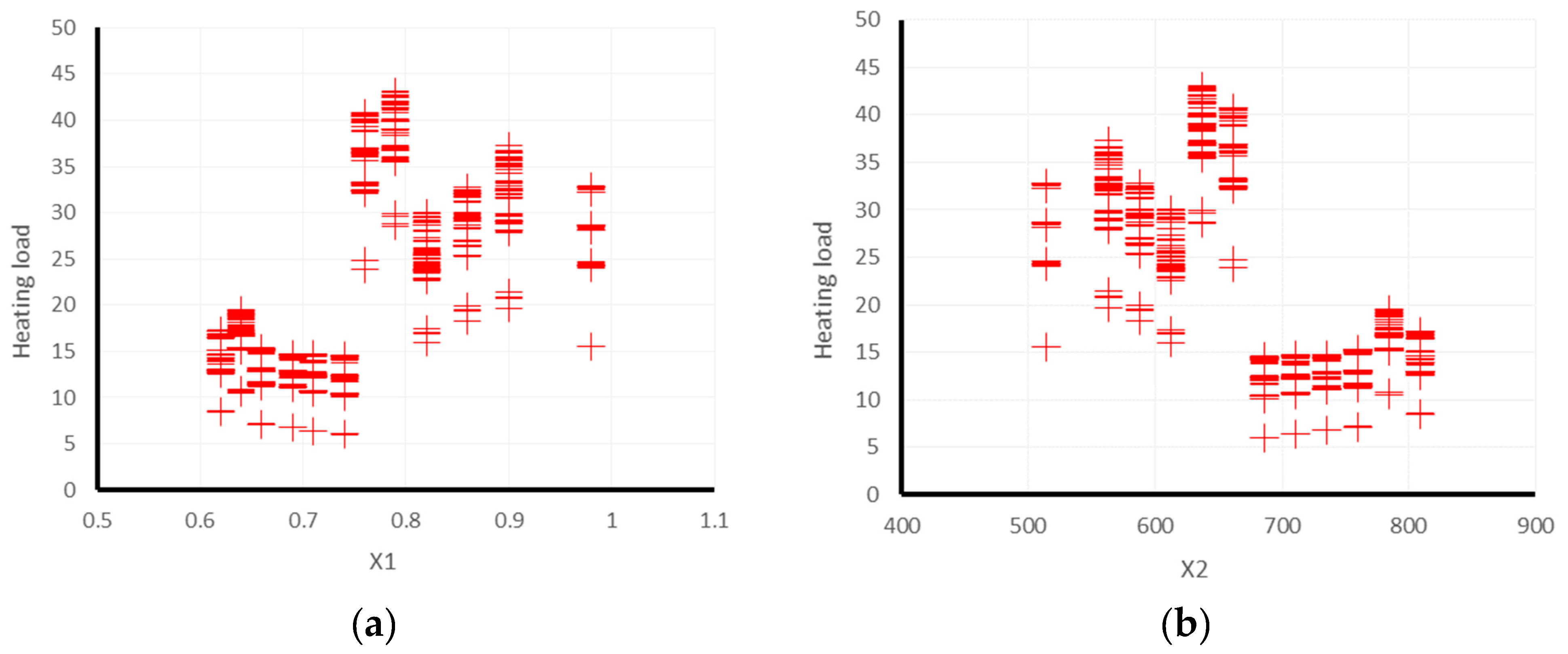
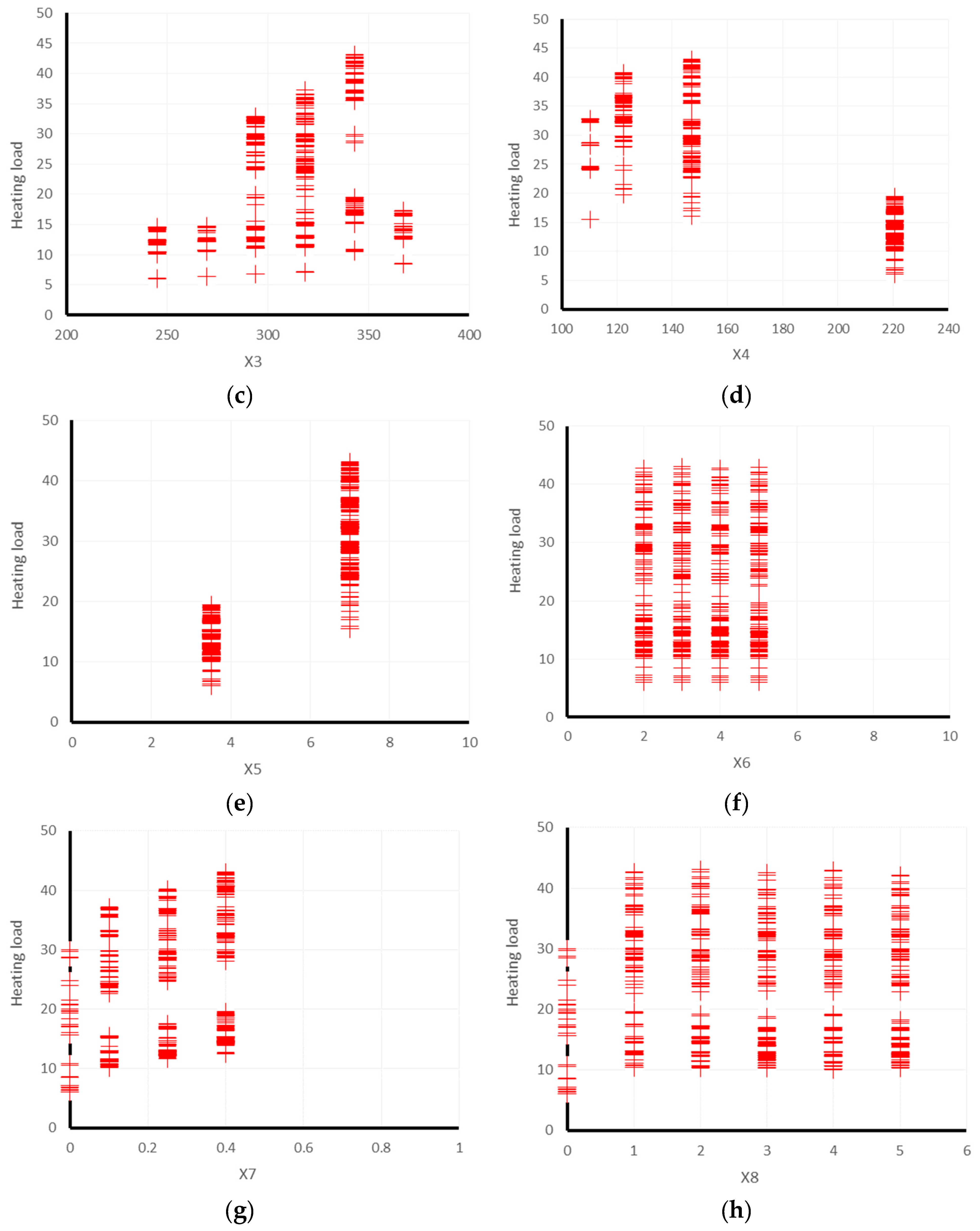
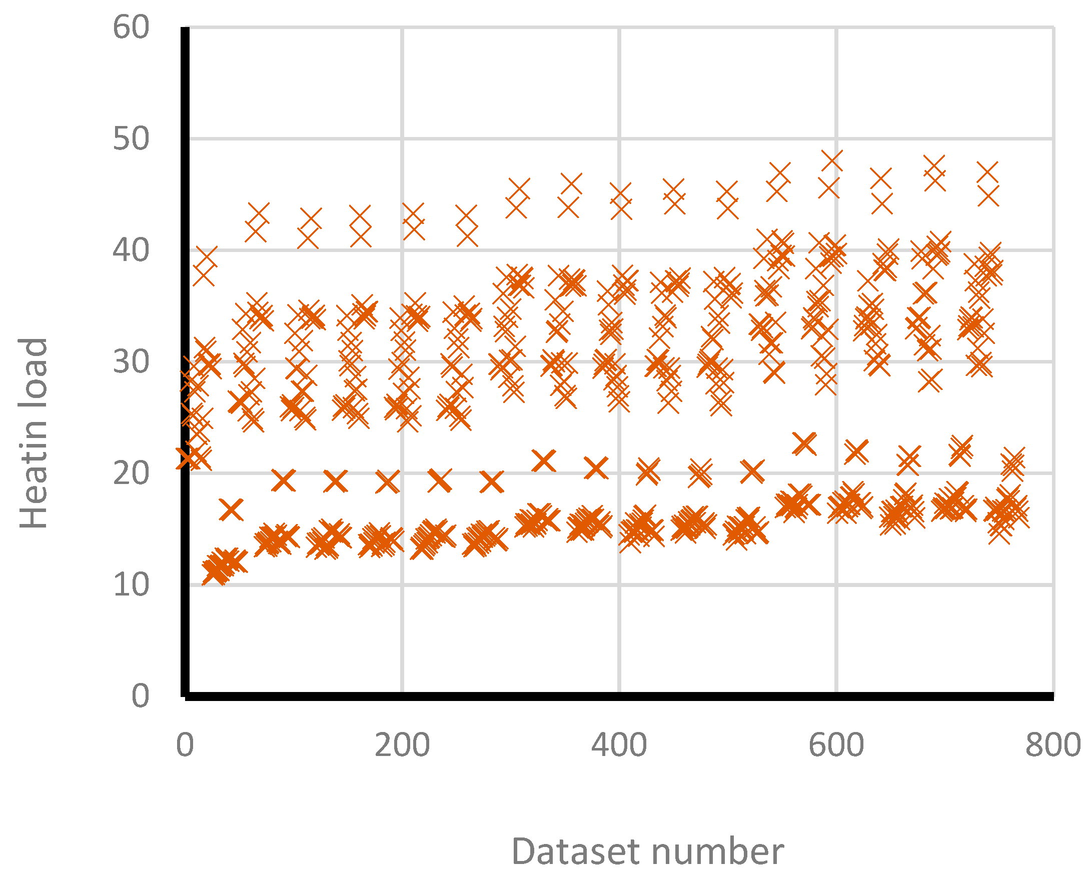
2. Database Collection

The required initial dataset was obtained from Tsanas and Xifara [43]. The obtained records include eight inputs (i.e., conditional factors) and a separate output of heating load (i.e., response factors or dependent outputs). Based on a residential building main conditional design factors, the inputs were X1 (Relative Compactness), X2 (Surface Area), X3 (Wall Area), X4 (Roof Area), X5 (Overall Height), X6 (Orientation), X7 (Glazing Area), and finally, X8 (Glazing Area Distribution). Likewise, parameters of the heating load of the suggested building were presented to be forecasted by the inputs. In addition, in this study the heating loads, as the main outputs, were simplified as heating load. The characteristics of the analyzed building and fundamental assumptions are properly detailed in the [43]. A total of 768 buildings were modelled considering twelve distinct buildings, five distribution scenarios, four orientations, and four glazing areas. The obtained data is analyzed through Ecotect computer software. A graphical view of this process is illustrated in Figure 1.

Statistical Details of the Dataset

As stated earlier, the amount of the heating load was applied as the main target of the energy-efficient buildings, while the main influential parameters were roof area, wall area, relative compactness, surface area, overall height, glazing area, glazing area distribution, and orientation. The statistical explanation of energy-efficient residential buildings including conditional variables is tabulated in Table 1. In addition, Figure 2 shows the variables of relative compactness, wall area, surface area, overall height, roof area, glazing area, orientation (i.e., north, northeast, east, southeast, south, southwest, west, northwest), heating load, and glazing area distribution on the x-axis, against a heating load (Figure 3) on the y-axis.

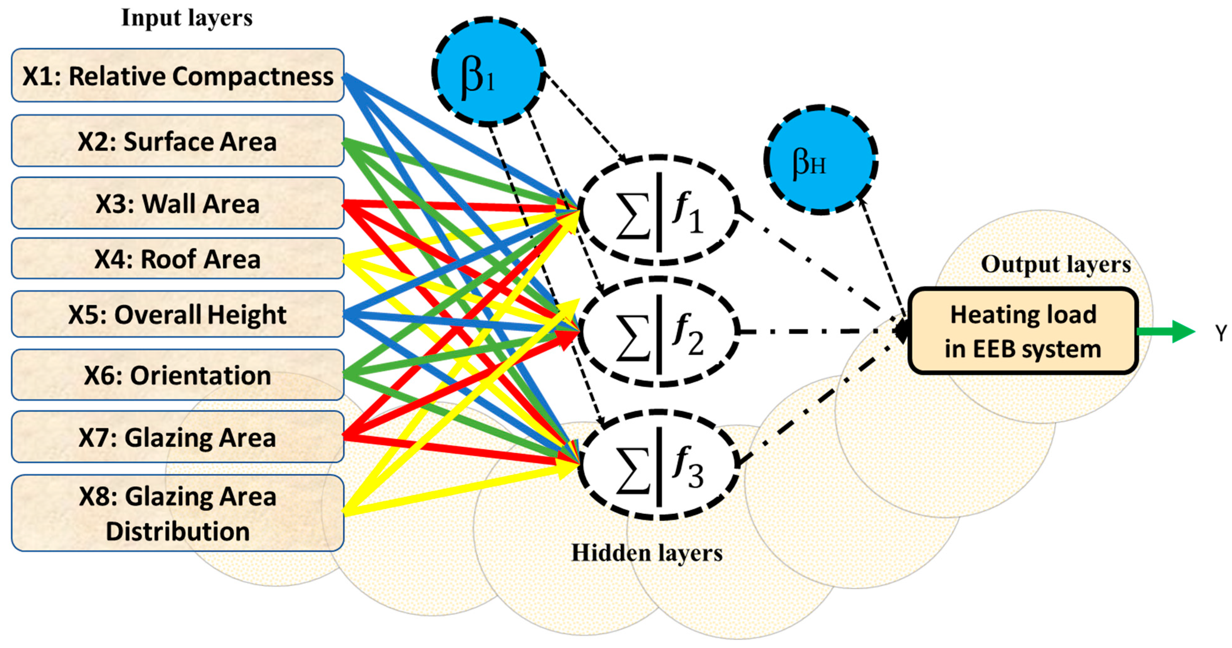
3. Model Development

An acceptable predict approach that is utilized with different artificial intelligence-based systems like MLPr, LLWL, AMT, RF, ENet, and RBFr models to predict heating load in energy-efficient buildings requires several steps. After that, the best fit model is then selected. Firstly, the initial database should be separated to the datasets of training (80% of the whole dataset) and testing (20% of the whole dataset). In the current study and because of the size of the testing dataset, the predictability of generated networks is considered to be as a proof of their validations. Therefore, a greater percentage of the dataset is considered for the testing dataset to be reliable for testing the trained network. Secondly, in order to obtain the best predictive network, appropriate machine learning-based solutions have to be introduced. Lastly, the outcome of the trained network should be validated and verified for selected testing datasets, randomly. The dataset utilized in this work is generated by some of the most influential input layers, such as surface area, roof area, relative compactness, wall area, glazing area, glazing area distribution, overall height, and orientation, which are the effective parameters influencing the heating load value in energy-efficient buildings. Note that the employed dataset was obtained from a recent study conducted by Tsanas and Xifara [43].
All six machine learning analyses provided in the current study were performed using Waikato Environment for Knowledge Analysis (WEKA). WEKA is a java-based open-source machine learning analyzer software that was developed in University of Waikato, New Zealand. Each of the proposed techniques were performed in optimized settings as explained in this section.

3.1. Multi-Layer Perceptron Regressor (MLPr)

The MLP is a widely-used and well-known predictive network. Accordingly, MLPr aims to coordinate the best potential of regression between a set of data samples (shown here in terms of S). The MLPr divides the S into both of the set training and testing databases. An MLP involves several layers of computational nodes. Similar to many previous MLPr-based studies, a single hidden layer was used. This is because even with a single hidden layer and increasing the number of nodes in the hidden layer an excellent rate of prediction can be achieved. Figure 4 shows a common MLP structure. The optimum number of neurons in each of the hidden layer are obtained after a series of trial and error processes (i.e., sensitivity analysis) as shown in Figure 5. Noteworthily, only one hidden layer was selected since the accuracy of a single hidden layer was found to be high enough to not make the MLP structure more complicated.
Each node generates a local output. In addition, it sets the local output to the subsequent layer (the next nodes in a further hidden layer) until reaching the nodes of output, i.e., the nodes placed in the layer of output. Equation (1) shows the normal operation carried out considering a dataset of N groups of records by the jth neuron to compute the predicted output:
O j = F   ( n = 1 N I n W n j + b j ) ,
where I symbolizes the input, b denotes the bias of the node, W is the weighting factor, and F signifies the activation function. Tansig (i.e., the tangent sigmoid activation function) is employed (Equation (2)). Note that we can have several types of activation functions (e.g., (i) sigmoid or logistic; (ii) Tanh—Hyperbolic tangent; (iii) Relu—rectified linear units) and that their performances are best suitable for different purposes. In the specific case of the sigmoid, this function (i) is real-valued and differentiable (i.e., to find gradients); (ii) has analytic tractability for the differentiation operation; and (iii) is an acceptable mathematical representation biological neuronal behavior.
T a n s i g ( x ) = 2 1 + e 2 x 1

3.2. Lazy Locally Weighted Learning (LLWL)

Similar to the K-star technique (i.e., an instance-based classifier), locally-weighted learning (LWL) [44] is one of the common types of lazy learning-based solutions. Lazy learning approaches provide valuable training algorithms and representations for learning about complex phenomena during autonomous adaptive control of complex systems. Commonly, there are disadvantages in employing such methods. Lazy learners create a considerable delay during the network simulation. More explanations about this model are provided by Atkeso, et al. [44].
The key options we have in LLWL include number of decimal places (numDecimalPlaces), batch size (batchSize), KNN (following the k-nearest neighbors algorithm), nearest neighbor search algorithm (nearestNeighborSearchAlgorithm), and weighting Kernel (weightingKernel). More explanations are provided below for each of the above influential parameters.
numDecimalPlaces—The number of decimal places. This number will be implemented for the output of numbers in the model.
batchSize—The chosen number of cases to process if batch estimation is being completed. A normal value of the batch size is 100. In this example we also consider it to be constant as it did not have significant impact on the outputs.
KNN—The number of neighbors that are employed to set the width of the weighting function (noting that KNN ≤ 0 means all neighbors are considered).
nearestNeighborSearchAlgorithm—The potential nearest neighbor search algorithm to be applied (the default algorithm that was also selected in our study was LinearNN).
weightingKernel—The number that determines the weighting function. (0 = Linear; 1 = Epnechnikov; 2 = Tricube; 3 = Inverse; 4 = Gaussian; and 5 = Constant. (default 0 = Linear)).
A good example of k-nearest neighbors algorithm is shown in Figure 6. The test sample (red dot) should be classified either as blue squares or as green triangles. If k = 3 (i.e., depicted in solid line circle) it is depicted by the green triangles as there are two triangles (reversed in shape) and only one rectangle through the inner (i.e., continuous line) circle. If k = 5 (dashed line circle) it is assigned to the blue rectangles (three blue rectangles vs. two green triangles inside the outer circle). Variation of the correlation coefficient (R2) versus number of used KNN neighbors is shown in Figure 7. It can be seen that changing the KNN could significantly enhance the correlation coefficient. For the cases of KNN = −1, KNN = 2, KNN = 4, KNN = 6, KNN = 8, and KNN =10, the training correlation coefficients were 0.9025, 0.9579, 0.9861, 0.9916, 0.9937, and 0.9943, respectively. In the case of our study we proposed the KNN = −1 as it considers all neighbors.

3.3. Alternating Model Tree (AMT)

Alternating model tree (AMT) [45] is supported by ensemble learning. In this technique, a single tree will form the structure of AMT. Therefore, it can be compared with the M5P tree algorithm (i.e., a reconstruction of Quinlan’s M5 algorithm for developing trees of regression models). It is well known that the M5P combines a conventional decision tree with the possibility of linear regression functions at the nodes. This model has been successfully employed in different subjects [46,47]. As the most similar technique with the AMT, alternating decision trees (ADT) provide the predictive power of decision tree ensembles in a single tree structure. Existing approaches for growing alternating decision trees focus on classification problems. In this paper, to find a relationship between the inputs and output layer we have proposed the AMT for regression, inspired by work on model trees for regression. As in most machine learning-based solutions, there are different parameters that can directly influence the accuracy of the prediction; we have run sensitivity analysis for different influential parameters. Since the highest variations in the results obtained stemmed from the term‘number of iterations’ we ran the analysis with different iteration numbers. To have a different data validation system, a new system of 10 k-fold selection was used here. It can be seen that the R2 reduces when the number of iterations increases. Therefore, the number of iterations equal to 10 was used as the default in the Weka software.
Some of the influential terms that can influence the accuracy of the regression are number of iterations (numberOfIterations), batch size (batchSize), and number of decimal places (numDecimalPlaces).
NumberOfIterations—Sets the number of iterations to perform. A sensitivity analysis is provided to select a proper number of iterations for the proposed AMT structure (as shown in Table 2 and Figure 8).
NumDecimalPlaces—Is as described in LLWL. Based on the required accuracy, up to two decimals are considered for final outputs.
BatchSize—The preferred number of instances to process. In the current study the default batch size of 100 is considered.

3.4. Random Forest (RF)

The random forest (RF) technique [48] is well known as an ensemble-learning solution that can be applied to regression as well as classification trees [49]. To improve the performance of classification trees, RF randomly alters the relations dealing with predictions. For providing the forest, some parameters (for example, the number of variables that split the nodes (g) and the number of trees (t)) need to be determined by the user. In this regard, the settings that were chosen for performing the RF techniques were as follows: seed = 1; number of execution slots = 1; number of decimal places = 2; the batch size = 100; the number of iterations = 100; the maximum depth = 0; should RF compute attribute importance = False; the number of features = 0. This technique has been employed and recommended as a good solution in numerous studies (Ho [50], Svetnik et al. [51], Diaz-Uriarte and de Andres [52], and Cutler et al. [53]).

3.5. ElasticNet (ENet)

To understand how ENet finds a solution, we need to make some assumptions. Consider a set of samples {(xi, yi), i = 1, 2, … N}, where each xiRp and yiR. Also, consider y = (y1, y2, …, yn)T and XRn×p as denoting the vector that is called “response vector” and the set design matrix, respectively. During the model analyzing, ENet (as described in Zou and Hastie [54]) establishes a linear program of two parameters (K1 and K2) to estimate the target. To do this, ENet should minimize the squared loss with K2-regularization and K1-norm constraint,
m i n β R p X β y 2 2 + μ 2 β 2 2   s u c h   t h a t   | β | 1 g ,
where β = [β1, β2, …, βZ]TRp denotes the weight vector, μ20 is the P2-regularization factor, and g > 0 represents by P1-norm budget. The K1 constraint encourages the method to be sparse. The presence of the K2 regularization factor causes the acquisition of a unique solution by making the problem severely convex, and if P N the optimization continues as stable for noticeable values of g. Furthermore, it helps the solution to be more stable when there is a high correlation between the features. For the number of the models (i.e., the set length of the lambda sequence to be generated), the value of 100 was used. For the number of decimal places (i.e., the number of decimal places to be used for the output of numbers in the model), as usual, the value of 2 was selected. The batch size was considered to be 100. The values of alpha and epsilon were set to be 0.001 and 0.0001, respectively. Along with the above-mentioned structure, a unique linear regression equation can also be found from the ENet as shown in Equation (4):
HL = −0.049 × X2 + 0.100 × X3 + −0.075 × X4 + 0.144 × X5 + −0.003 × X6 + 0.051 × X7 +
0.161 × X8 + 35.597.

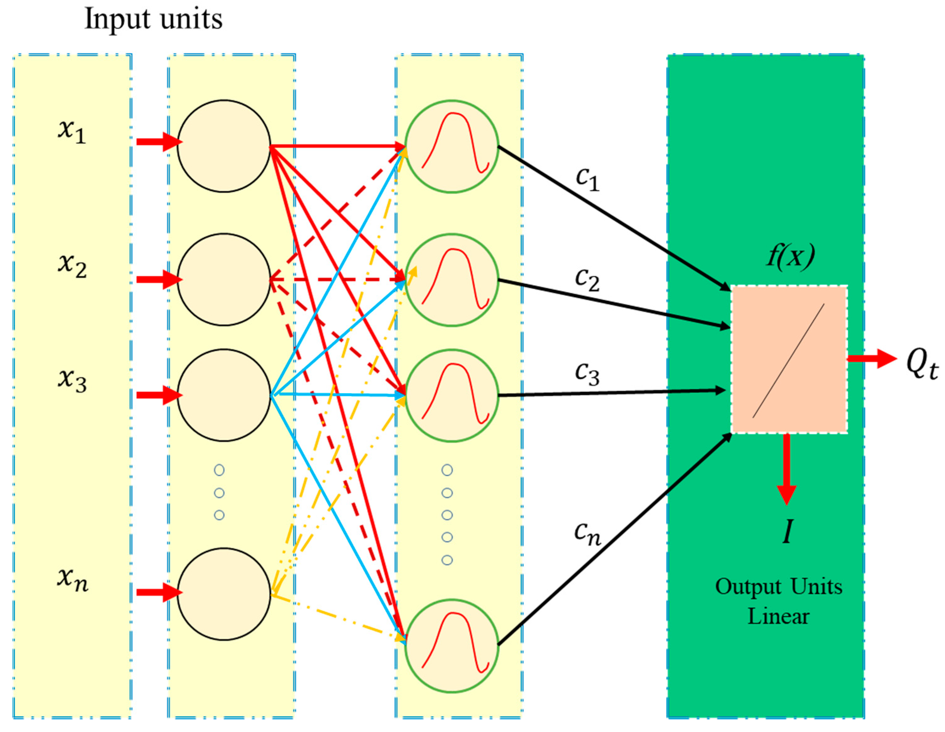
3.6. Radial Basis Function Regression (RBFr)

Radial basis function network (RBFr) has a unique structure, as explained in Figure 9. Equation (5) illustrates the basis function of this network [55]. For solving the issue, radial basis function regression can be used by fitting a collection of kernels for the dataset. In addition, this method attends the position of noisy samples.
O i = K ( x x i τ i 2 )
Oi stands for the output of the neuron, and xi shows the center of kernel K. in addition, the term τ i stands for the width of the ith RBF unit.
The model of RBFr utilizes a bath algorithm for predicting the number of developed kernels. This prediction is performed by bath algorithms. The specific function of expectation that is utilized in RBFR model is as below:
F ( x ) = i = 1 z k ( x x i )   φ i .
x stands to symbolize the Euclidean norm on x . { k ( x x i ) |   i = 1 , 2 , , z } stands as a group of z non-linear along with constant RBFr. In addition, the term φ i shows the coefficient of regression.

3.7. Model Assessment Approaches

To evaluate the reliability of early estimated heating load in energy-efficient residential buildings, five well-known (as used mostly in academic studies) statistical indices including root mean square error (RMSE, relative absolute error (RAE in %, mean absolute error (MAE), root relative squared error (RRSE in %) and coefficient of determination (R2) are used to help to rank the network performances. The outputs of these statistical indexes are also used for color intensity ranking. Equations (7)–(11) designate the equations of R2, MAE, RMSE, RAE, and RRSE, respectively.
R 2 = 1 i = 1 s ( Y i p r e d i c t e d Y i o b s e r v e d ) 2 i = 1 s ( Y i o b s e r v e d Y ¯ o b s e r v e d ) 2 ,
M A E = 1 N I = 1 s | Y i o b s e r v e d Y i p r e d i c t e d | ,
R M S E = 1 N i = 1 s [ ( Y i o b s e r v e d Y i p r e d i c t e d ) ] 2 ,
R A E = i = 1 s | Y i p r e d i c t e d Y i o b s e r v e d | i = 1 s | Y i o b s e r v e d Y ¯ o b s e r v e d | ,
R R S E = i = 1 s ( Y i p r e d i c t e d Y i o b s e r v e d ) 2 i = 1 s ( Y i o b s e r v e d Y ¯ o b s e r v e d ) 2 ,
where, Y i o b s e r v e d and Y i p r e d i c t e d , represented in Equations (6) to (10), are the actual and estimated values of heating load in energy-efficient buildings, respectively. The term S in the above equations stands for the number of instances and Y ¯ observed denotes the mean of the real amounts of the heating load. Weka software environment was employed to perform the machine learning models.

4. Results and Discussion

The present research aimed to provide a reliable early estimation of the heating load in energy-efficient building systems through several machine learning solutions, namely MLPr, LLWL, AMT, RF, ENet, and RBFr models. These approaches are well known. After running all these machine learning techniques, the best outputs can be selected as the most trustworthy solutions in the early estimation of heating load in energy-efficient residential buildings. Therefore, to find the most appropriate predictive networks, the proposed AI models (e.g., MLPr, LLWL, AMT, RF, ENet, and RBFr models) are evaluated and compared. The results of employed machine learning-based solutions proposed here, and their performances are evaluated through Table 3 and Table 4. The overall scoring for the performances of the proposed technique is provided further in Table 5.
As is illustrated Figure 10 and Figure 11, AMT, RF, and MLPr models provided significant accuracy in predicting heating load in energy-efficient buildings, however, the RF-based model can be nominated as more reliable than other developed estimations of machine learning-based techniques. The values 10, 25, 30, 5, 20, and 15 were calculated as the total scores for the LLWL, ATM, RF, ENet, MLPr, and RBFr techniques, respectively. These scores prove the superiority of the RF when compared with other nominated models. The amounts of R2, MAE, RMSE, RAE (%), and RRSE (%) in the RF model for the training dataset were 0.9997, 0.19, 0.2399, 2.078, and 2.3795, respectively. The amounts of R2, MAE, RMSE, RAE (%), and RRSE (%) in the RF model for the testing dataset were 0.9989, 0.3385, 0.4649, 3.6813, and 4.5995, respectively. This indicates the higher reliability of the generated RF method compared to other techniques. The weakest estimation model results were from ENet solution where the R2, MAE, RMSE, RAE (%), and RRSE (%) were 0.8915, 3.2332, 4.5678, 35.3566, and 45.2993 in the training dataset, respectively, and the R2, MAE, RMSE, RAE (%), and RRSE (%) were 0.896, 3.2585, 4.4683, 35.4392, and 44.2052 for the testing dataset, respectively. According to the total scoring, the best performance from Table 4 was found to be RF. Right after RF model, the next best estimation network was obtained for the AMT technique. The R2, MAE, RMSE, RAE (%), and RRSE (%) for the AMT training dataset were 0.9985, 0.4096, 0.5449, 4.4788, and 5.4036, respectively. The R2, MAE, RMSE, RAE (%), and RRSE (%) for the AMT testing dataset were 0.9981, 0.4869, 0.6236, 5.2956, and 6.1693, respectively.
The results of network reliability based on the R2 performance of all proposed models, for both training and testing, are provided in Figure 10 and Figure 11. As stated earlier, both of the RF models could provide a more reliable predictive network with higher accuracy when compared to other proposed techniques. The results of network output for the proposed RF are illustrated in Figure 10d and Figure 11d. Having the provided information, the predictive network of RF proved to be slightly better than other proposed techniques and was superior in making a better regression relationship among the estimated and actual values.

5. Conclusions

In the current study, several predictive networks were introduced and evaluated. The study aimed to assess and compare several of the most well-known machine learning-based techniques in order to introduce the most reliable predictive method in early estimation of heating load in energy-efficient residential building systems. Machine learning-based solutions, namely, MLPr, LLWL, AMT, RF, ENet, and RBFr models were employed to estimate the heating load. The results of the best model from the proposed techniques were presented. Based on the presented outcomes, it may be said that, except for the ENet model, almost all models (i.e., MLPr, LLWL, AMT, RF, and RBFr) have good prediction output results in estimating heating load in energy-efficient building systems. In this regard, the RF machine learning technique could be suggested as the most reliable and accurate among other predictive techniques provided in the present work. The learning approach is good in RF predictive models when compared to other models concerning both the training and validation models. The values of R2, MAE, RMSE, RAE (%), and RRSE (%) in the RF model training dataset, were 0.9997, 0.19, 0.2399, 2.078, and 2.3795, respectively. The values of R2, MAE, RMSE, RAE (%), and RRSE (%) in the AMT model training dataset were 0.9985, 0.4096, 0.5449, 4.4788, and 5.4036, respectively. Validated testing datasets from the selected techniques also showed appropriate accuracy as R2, MAE, RMSE, RAE (%), and RRSE (%) in the testing output of the RF model were found to be 0.9989, 0.3385, 0.4649, 3.6813, and 4.5995, respectively; R2, MAE, RMSE, RAE (%), and RRSE (%) in the testing output of the AMT model were found to be 0.9981, 0.4869, 0.6236, 5.2956, and 6.1693, respectively. The worst validation was found for the ENet technique with R2, MAE, RMSE, RAE (%), and RRSE (%) equal to 0.896, 3.2585, 4.4683, 35.4392, and 44.2052, respectively.

Author Contributions

H.M., D.T.B., A.D. wrote the manuscript, discussion and analyzed the data. H.M. and A.D., Z.L., and L.K.F. edited, restructured, and professionally optimized the manuscript.

Funding

This study was funded by the Ton Duc Thang University and University of South-Eastern Norway.

Conflicts of Interest

The authors declare no conflict of interest.

References

  1. Nguyen, T.N.; Tran, T.P.; Hung, H.D.; Voznak, M.; Tran, P.T.; Minh, T.; Thanh-Long, N. Hybrid TSR-PSR alternate energy harvesting relay network over Rician fading channels: Outage probability and SER analysis. Sensors 2018, 18, 3839. [Google Scholar] [CrossRef]
  2. Najafi, B.; Ardabili, S.F.; Mosavi, A.; Shamshirband, S.; Rabczuk, T. An intelligent artificial neural network-response surface methodology method for accessing the optimum biodiesel and diesel fuel blending conditions in a diesel engine from the viewpoint of exergy and energy analysis. Energies 2018, 11, 860. [Google Scholar] [CrossRef]
  3. Nazir, R.; Ghareh, S.; Mosallanezhad, M.; Moayedi, H. The influence of rainfall intensity on soil loss mass from cellular confined slopes. Measurement 2016, 81, 13–25. [Google Scholar] [CrossRef]
  4. Mojaddadi, H.; Pradhan, B.; Nampak, H.; Ahmad, N.; Ghazali, A.H.B. Ensemble machine-learning-based geospatial approach for flood risk assessment using multi-sensor remote-sensing data and GIS. Geomat. Nat. Hazards Risk 2017, 8, 1080–1102. [Google Scholar] [CrossRef] [Green Version]
  5. Rizeei, H.M.; Pradhan, B.; Saharkhiz, M.A. Allocation of emergency response centres in response to pluvial flooding-prone demand points using integrated multiple layer perceptron and maximum coverage location problem models. Int. J. Disaster Risk Reduct. 2019, 101205. [Google Scholar] [CrossRef]
  6. Rizeei, H.M.; Pradhan, B.; Saharkhiz, M.A. Urban object extraction using Dempster Shafer feature-based image analysis from worldview-3 satellite imagery. Int. J. Remote Sens. 2019, 40, 1092–1119. [Google Scholar] [CrossRef]
  7. Mezaal, M.; Pradhan, B.; Rizeei, H. Improving landslide detection from airborne laser scanning data using optimized Dempster–Shafer. Remote Sens. 2018, 10, 1029. [Google Scholar] [CrossRef]
  8. Aal-shamkhi, A.D.S.; Mojaddadi, H.; Pradhan, B.; Abdullahi, S. Extraction and modeling of urban sprawl development in Karbala City using VHR satellite imagery. In Spatial Modeling and Assessment of Urban Form; Springer: Cham, Switzerland, 2017; pp. 281–296. [Google Scholar]
  9. Gao, W.; Wang, W.; Dimitrov, D.; Wang, Y. Nano properties analysis via fourth multiplicative ABC indicator calculating. Arab. J. Chem. 2018, 11, 793–801. [Google Scholar] [CrossRef]
  10. Aksoy, H.S.; Gör, M.; İnal, E. A new design chart for estimating friction angle between soil and pile materials. Geomech. Eng. 2016, 10, 315–324. [Google Scholar] [CrossRef]
  11. Gao, W.; Dimitrov, D.; Abdo, H. Tight independent set neighborhood union condition for fractional critical deleted graphs and ID deleted graphs. Discret. Contin. Dyn. Syst. S 2018, 12, 711–721. [Google Scholar] [CrossRef]
  12. Bui, D.T.; Moayedi, H.; Gör, M.; Jaafari, A.; Foong, L.K. Predicting slope stability failure through machine learning paradigms. ISPRS Int. Geo-Inf. 2019, 8, 395. [Google Scholar] [CrossRef]
  13. Gao, W.; Guirao, J.L.G.; Abdel-Aty, M.; Xi, W. An independent set degree condition for fractional critical deleted graphs. Discret. Contin. Dyn. Syst. S 2019, 12, 877–886. [Google Scholar] [CrossRef] [Green Version]
  14. Moayedi, H.; Bui, D.T.; Gör, M.; Pradhan, B.; Jaafari, A. The feasibility of three prediction techniques of the artificial neural network, adaptive neuro-fuzzy inference system, and hybrid particle swarm optimization for assessing the safety factor of cohesive slopes. ISPRS Int. Geo-Inf. 2019, 8, 391. [Google Scholar] [CrossRef]
  15. Gao, W.; Guirao, J.L.G.; Basavanagoud, B.; Wu, J. Partial multi-dividing ontology learning algorithm. Inf. Sci. 2018, 467, 35–58. [Google Scholar] [CrossRef]
  16. Ince, R.; Gör, M.; Alyamaç, K.E.; Eren, M.E. Multi-fractal scaling law for split strength of concrete cubes. Mag. Concr. Res. 2016, 68, 141–150. [Google Scholar] [CrossRef]
  17. Gao, W.; Wu, H.; Siddiqui, M.K.; Baig, A.Q. Study of biological networks using graph theory. Saudi J. Biol. Sci. 2018, 25, 1212–1219. [Google Scholar] [CrossRef]
  18. Ngo, N.T. Early predicting cooling loads for energy-efficient design in office buildings by machine learning. Energy Build. 2019, 182, 264–273. [Google Scholar] [CrossRef]
  19. Jafarinejad, T.; Erfani, A.; Fathi, A.; Shafii, M.B. Bi-level energy-efficient occupancy profile optimization integrated with demand-driven control strategy: University building energy saving. Sustain. Cities Soc. 2019, 48, 101539. [Google Scholar] [CrossRef]
  20. Kheiri, F. A review on optimization methods applied in energy-efficient building geometry and envelope design. Renew. Sustain. Energy Rev. 2018, 92, 897–920. [Google Scholar] [CrossRef]
  21. Wang, W.; Chen, J.Y.; Huang, G.S.; Lu, Y.J. Energy efficient HVAC control for an IPS-enabled large space in commercial buildings through dynamic spatial occupancy distribution. Appl. Energy 2017, 207, 305–323. [Google Scholar] [CrossRef]
  22. Yu, Z.; Haghighat, F.; Fung, B.C.M. Advances and challenges in building engineering and data mining applications for energy-efficient communities. Sustain. Cities Soc. 2016, 25, 33–38. [Google Scholar] [CrossRef] [Green Version]
  23. Zhang, H.; Yuan, C.; Yang, G.; Wu, L.; Peng, C.; Ye, W.; Shen, Y.; Moayedi, H. A novel constitutive modelling approach measured under simulated freeze–thaw cycles for the rock failure. Eng. Comput. 2019. [Google Scholar] [CrossRef]
  24. Bui, D.T.; Moayedi, H.; Anastasios, D.; Foong, L.K. Predicting heating and cooling loads in energy-efficient buildings using two hybrid intelligent models. Appl. Sci. 2019, 9, 3543. [Google Scholar]
  25. Moayedi, H.; Nguyen, H.; Rashid, A.S.A. Comparison of dragonfly algorithm and Harris hawks optimization evolutionary data mining techniques for the assessment of bearing capacity of footings over two-layer foundation soils. Eng. Comput. 2019. [Google Scholar] [CrossRef]
  26. Moayedi, H.; Aghel, B.; Abdullahi, M.A.M.; Nguyen, H.; Rashid, A.S.A. Applications of rice husk ash as green and sustainable biomass. J. Clean. Prod. 2019, 237, 117851. [Google Scholar] [CrossRef]
  27. Huang, X.X.; Moayedi, H.; Gong, S.; Gao, W. Application of metaheuristic algorithms for pressure analysis of crude oil pipeline. Energy Sources Part A Recovery Util. Environ. Effects 2019. [Google Scholar] [CrossRef]
  28. Gao, W.; Alsarraf, J.; Moayedi, H.; Shahsavar, A.; Nguyen, H. Comprehensive preference learning and feature validity for designing energy-efficient residential buildings using machine learning paradigms. Appl. Soft Comput. 2019, 84, 105748. [Google Scholar] [CrossRef]
  29. Bui, D.T.; Moayedi, H.; Kalantar, B.; Osouli, A.; Pradhan, B.; Nguyen, H.; Rashid, A.S.A. Harris hawks optimization: A novel swarm intelligence technique for spatial assessment of landslide susceptibility. Sensors 2019, 19, 3590. [Google Scholar] [CrossRef]
  30. Biswas, M.R.; Robinson, M.D.; Fumo, N. Prediction of residential building energy consumption: A neural network approach. Energy 2016, 117, 84–92. [Google Scholar] [CrossRef]
  31. Fan, C.; Wang, J.; Gang, W.; Li, S. Assessment of deep recurrent neural network-based strategies for short-term building energy predictions. Appl. Energy 2019, 236, 700–710. [Google Scholar] [CrossRef]
  32. Ince, R.; Gör, M.; Eren, M.E.; Alyamaç, K.E. The effect of size on the splitting strength of cubic concrete members. Strain 2015, 51, 135–146. [Google Scholar] [CrossRef]
  33. Sayin, E.; Yön, B.; Calayir, Y.; Gör, M. Construction failures of masonry and adobe buildings during the 2011 Van earthquakes in Turkey. Struct. Eng. Mech. 2014, 51, 503–518. [Google Scholar] [CrossRef]
  34. Zemella, G.; de March, D.; Borrotti, M.; Poli, I. Optimised design of energy efficient building facades via evolutionary neural networks. Energy Build. 2011, 43, 3297–3302. [Google Scholar] [CrossRef]
  35. Chou, J.S.; Bui, D.K. Modeling heating and cooling loads by artificial intelligence for energy-efficient building design. Energy Build. 2014, 82, 437–446. [Google Scholar] [CrossRef]
  36. Hidayat, I.; Utami, S.S. Activity based smart lighting control for energy efficient building by neural network model. In Astechnova 2017 International Energy Conference; Sunarno, I., Sasmito, A.P., Hong, L.P., Eds.; EDP Sciences: Les Ulis, France, 2018; Volume 43. [Google Scholar]
  37. Malik, S.; Kim, D. Prediction-learning algorithm for efficient energy consumption in smart buildings based on particle regeneration and velocity boost in particle swarm optimization neural networks. Energies 2018, 11, 1289. [Google Scholar] [CrossRef]
  38. Pino-Mejías, R.; Pérez-Fargallo, A.; Rubio-Bellido, C.; Pulido-Arcas, J.A. Comparison of linear regression and artificial neural networks models to predict heating and cooling energy demand, energy consumption and CO2 emissions. Energy 2017, 118, 24–36. [Google Scholar] [CrossRef]
  39. Deb, C.; Eang, L.S.; Yang, J.; Santamouris, M. Forecasting diurnal cooling energy load for institutional buildings using artificial neural networks. Energy Build. 2016, 121, 284–297. [Google Scholar] [CrossRef]
  40. Li, Q.; Meng, Q.; Cai, J.; Yoshino, H.; Mochida, A. Predicting hourly cooling load in the building: A comparison of support vector machine and different artificial neural networks. Energy Convers. Manag. 2009, 50, 90–96. [Google Scholar] [CrossRef]
  41. Kolokotroni, M.; Davies, M.; Croxford, B.; Bhuiyan, S.; Mavrogianni, A. A validated methodology for the prediction of heating and cooling energy demand for buildings within the Urban Heat Island: Case-study of London. Sol. Energy 2010, 84, 2246–2255. [Google Scholar] [CrossRef] [Green Version]
  42. Nguyen, H.; Moayedi, H.; Foong, L.K.; Al Najjar, H.A.H.; Jusoh, W.A.W.; Rashid, A.S.A.; Jamali, J. Optimizing ANN models with PSO for predicting short building seismic response. Eng. Comput. 2019, 35, 1–15. [Google Scholar] [CrossRef]
  43. Tsanas, A.; Xifara, A. Accurate quantitative estimation of energy performance of residential buildings using statistical machine learning tools. Energy Build. 2012, 49, 560–567. [Google Scholar] [CrossRef]
  44. Atkeson, C.G.; Moore, A.W.; Schaal, S. Locally weighted learning for control. In Lazy Learning; Springer: Dordrecht, The Netherlands, 1997; pp. 75–113. [Google Scholar]
  45. Frank, E.; Mayo, M.; Kramer, S. Alternating model trees. In Proceedings of the 30th Annual ACM Symposium on Applied Computing, Salamanca, Spain, 13–17 April 2015; pp. 871–878. [Google Scholar]
  46. Hamilton, C.R. Hourly Solar Radiation Forecasting through Neural Networks and Model Trees. Ph.D. Thesis, University of Georgia, Athens, GA, USA, 2016. [Google Scholar]
  47. Rodrigues, É.O.; Pinheiro, V.; Liatsis, P.; Conci, A. Machine learning in the prediction of cardiac epicardial and mediastinal fat volumes. Comput. Biol. Med. 2017, 89, 520–529. [Google Scholar] [CrossRef] [PubMed]
  48. Breiman, L. Random forests. Mach. Learn. 2001, 45, 5–32. [Google Scholar] [CrossRef]
  49. Breiman, L.; Friedman, J.H.; Olshen, R.A.; Stone, C.J. Classification and Regression Trees; Wadsworth International Group: Belmont, CA, USA, 1984. [Google Scholar]
  50. Ho, T.K. The random subspace method for constructing decision forests. IEEE Trans. Pattern Anal. Mach. Intell. 1998, 20, 832–844. [Google Scholar]
  51. Svetnik, V.; Liaw, A.; Tong, C.; Culberson, J.C.; Sheridan, R.P.; Feuston, B.P. Random forest: A classification and regression tool for compound classification and QSAR modeling. J. Chem. Inf. Comput. Sci. 2003, 43, 1947–1958. [Google Scholar] [CrossRef] [PubMed]
  52. Diaz-Uriarte, R.; de Andres, S.A. Gene selection and classification of microarray data using random forest. BMC Bioinform. 2006, 7, 3. [Google Scholar] [CrossRef]
  53. Cutler, D.R.; Edwards, T.C.; Beard, K.H.; Cutler, A.; Hess, K.T. Random forests for classification in ecology. Ecology 2007, 88, 2783–2792. [Google Scholar] [CrossRef]
  54. Zou, H.; Hastie, T. Regularization and variable selection via the elastic net. J. R. Stat. Soc. Ser. B (Stat. Methodol.) 2005, 67, 301–320. [Google Scholar] [CrossRef] [Green Version]
  55. Buhmann, M.D. Radial Basis Functions: Theory and Implementations; Cambridge University Press: Cambridge, UK, 2003; Volume 12. [Google Scholar]
Figure 1. Graphical view of data preparation.
Applsci 09 04338 g001
Figure 2. Schematic view of some of the input data layers (X1–X8 as shown in Table 1) in predicting heating load. (a) X1 (Relative Compactness); (b) X2 (Surface Area); (c) X3 (Wall Area); (d) X4 (Roof Area); (e) X5 (Overall Height); (f) X6 (Orientation); (g) X7 (Glazing Area); (h) X8 (Glazing Area Distribution).
Applsci 09 04338 g002aApplsci 09 04338 g002b
Figure 3. Schematic view of some of the output data layers (i.e., heating load).
Applsci 09 04338 g003
Figure 4. Multi-layer perceptron regressor (MLPr) neural network typical architecture.
Applsci 09 04338 g004
Figure 5. Sensitivity analysis based on number of neurons in a single hidden layer.
Applsci 09 04338 g005
Figure 6. Example of k-nearest neighbors (KNN) regression/classification.
Applsci 09 04338 g006
Figure 7. Variation of the correlation coefficient (R2) versus number of used KNN neighbors in lazy locally weighted learning (LLWL) technique.
Applsci 09 04338 g007
Figure 8. Variation of the correlation coefficient (R2) versus number of iterations, in alternating model tree (AMT) technique.
Applsci 09 04338 g008
Figure 9. Typical architecture of radial basis function regression (RBFr) neural network.
Applsci 09 04338 g009
Figure 10. The network outputs for the training dataset. (a) MLPr; (b) LLWL; (c) AMT; (d) RF; (e) ENet; (f) RBFr.
Applsci 09 04338 g010
Figure 11. The network outputs for the testing dataset. (a) MLPr; (b) LLWL; (c) AMT; (d) RF; (e) ENet; (f) RBFr.
Applsci 09 04338 g011
Table 1. The statistical description details in term of energy-efficient design.
Data Layers Used as InputMain Output
Relative Compactness Surface Area (m2)Wall Area (m2)Roof Area (m2)Overall Height (m)Orientation
(-)
Glazing Area (m2)Glazing Area Distribution (m2)Heating Load (kW/h)
Used labelX1X2X3X4X5X6X7X8Y1
No. of data768
Minimum0.6514.5245.0110.33.52.00.00.06.0
Maximum1.0808.5416.5220.57.05.00.45.043.1
Average0.8671.7318.5176.65.33.50.22.822.3
Table 2. Evaluation metrics calculated for the alternating model tree (AMT) method varied based on number of iterations.
Number of Iterations
Evaluation metrics1020304050
Correlation coefficient0.99840.99710.99740.99750.9972
Mean absolute error0.43490.75270.70510.64640.6666
Root mean squared error0.57520.95660.89360.84950.8995
Relative absolute error (%)4.757.947.436.827.0341
Root relative squared error (%)5.698.948.357.938.4062
Table 3. The performance of selected machine learning techniques in the prediction of heating load through several statistical indexes (training dataset).
Proposed ModelsNetwork ResultsRanking the Predicted ModelsTotal Ranking ScoreRank
R2MAERMSERAE (%)RRSE (%)R2MAERMSERAE (%)RRSE (%)
lazy.LWL0.9033.28384.333535.910442.97572121285
Alternating Model Tree0.99850.40960.54494.47885.403655555252
Random Forest0.99970.190.23992.0782.379566666301
ElasticNet0.89153.23324.567835.356645.29931212176
MLP Regressor0.99150.97951.315610.711713.046544444203
RBF Regressor0.96471.82262.655519.930726.334833333154
Table 4. The performance of selected machine learning techniques in the prediction of heating load through several statistical indexes (testing dataset).
Proposed ModelsNetwork ResultsRanking the Predicted ModelsTotal Ranking ScoreRank
R2MAERMSERAE (%)RRSE (%)R2MAERMSERAE (%)RRSE (%)
lazy.LWL0.90493.23454.275235.177842.295322222105
Alternating Model Tree0.99810.48690.62365.29566.169355555252
Random Forest0.99890.33850.46493.68134.599566666301
ElasticNet0.8963.25854.468335.439244.20521111156
MLP Regressor0.98681.121.626712.181116.093444444203
RBF Regressor0.96931.91092.464720.782724.383733333154
Table 5. Total ranking of proposed machine learning solutions.
Proposed ModelsTraining DatasetTesting DatasetTotal Rank
R2MAERMSERAE (%)RRSE (%)R2MAERMSERAERRSE
lazy.LWL212122222210
Alternating Model Tree555555555525
Random Forest666666666630
ElasticNet12121111115
MLP Regressor444444444420
RBF Regressor333333333315
RMSE: root mean squared error; R2: correlation coefficient; RRSE: root relative squared error; MAE: mean absolute error; RAE: relative absolute error.

