Economic Routing of Electric Vehicles using Dynamic Pricing in Consideration of System Voltage

Abstract

There is a growing market for electric vehicles (EVs) in recent years. Due to this, many studies on electric vehicles are in progress and research on charging operations for EVs are especially active. Recent research trends on electric vehicle routes rely on the stochastic modelling of various factors such as convenience of a user’s point of view, charging station (CS), location, destination, and so on. In this paper, a charging control scheme for electric vehicles is proposed from the point of view of the system operators rather than the user. From a user’s point of view, the EV route can be set up directly, but it is difficult for the system operator to directly participate in the route of the EV. In this paper, a method is proposed to indirectly change the route of the EV by changing the charging cost through real-time dynamic pricing, in order to prevent risks in the system operation due to voltage fluctuations in the system. With dynamic pricing, the voltage of the system is kept within a stable range, and the EV user sets the route with an economic benefit. The proposed scheme is verified through Dijkstra’s algorithm and a control strategy via a simulation model using MATLAB.

1. Introduction

Recently, there have been rising global efforts towards reducing greenhouse gas emissions. There are various regulations on carbon dioxide, which is the main cause of greenhouse gas emissions, and there is a lot of interest in technologies with lower carbon dioxide footprints. As a result, environment-friendly technologies and products such as electric vehicles (EVs) and renewable energy are attracting attention as countermeasures against rising global greenhouse gases. So far, most of the research related to EV routes has dealt with the convenience to electric vehicle users. In addition, the main research focus has been on finding a route that enhances a user’s convenience by considering a Markov chain using a probabilistic model [1,2]. Research on route setting mainly consists of a probabilistic model of the user’s pattern that is optimized considering various cost aspects according to the model [3]. Optimal charging of an EV on the user side is an efficient method because it sets the optimal route for a user’s purpose. However, this method has the disadvantage that as the number of EVs increases, various problems can arise in the power system.

As EV infrastructure continues to grow, there are more active data on the operations of charging stations [4,5,6]. In [4], an operating method is introduced that plans to charge in a highway environment and minimize total travel time. In [5], an operation that minimizes costs is suggested, including the cost of a power supply to EVs and the uncertainty of renewable energy. In [6], a charging strategy between charging stations (CSs) is proposed to reduce EV charging waiting time by considering traffic information and the statuses of CSs.

The purpose of this paper is to improve the issue of system voltage without compromising the convenience to the users, which is proposed by setting the route as the minimum charging cost for the EV while necessarily keeping the system stable and meeting the charging demands of electric vehicles. A control strategy for CSs with dynamic pricing is proposed in which the system operator shares information on charging schedules and pricing information between the charging stations and EVs and measures the voltage regulation of the system through the shared information. In response to voltage regulation, a price signal is sent to the charging station as dynamic pricing. Then, the EV resets the route to reflect the charging price information of the CS. In Section 2, the proposed routing algorithm for EVs is presented using Dijkstra’s algorithm. A control scheme for the CS and operator is presented in Section 3, and the simulation results for the control strategy are presented in Section 4. The control method proposed in this paper is verified using MATLAB.

2. EV Routing using Dijkstra’s Algorithm

Dijkstra’s algorithm finds the shortest path in a directed graph without negative weights. Shortest path implies a path that has the smallest sum of weights among the paths that can move from one point to another [7,8]. There are no negative weights, because the path can be reduced by running Dijkstra’s algorithm infinitely over a negative cycle [9]. The path with the minimum cost presented in this paper can be obtained using the weight of Dijkstra’s algorithm. If the weight of Dijkstra’s algorithm is converted to cost, the route with the smallest weight can be considered the route with the minimum cost. In this paper, weight implies the shortest time, the minimum distance, or the minimum cost according to objective function.

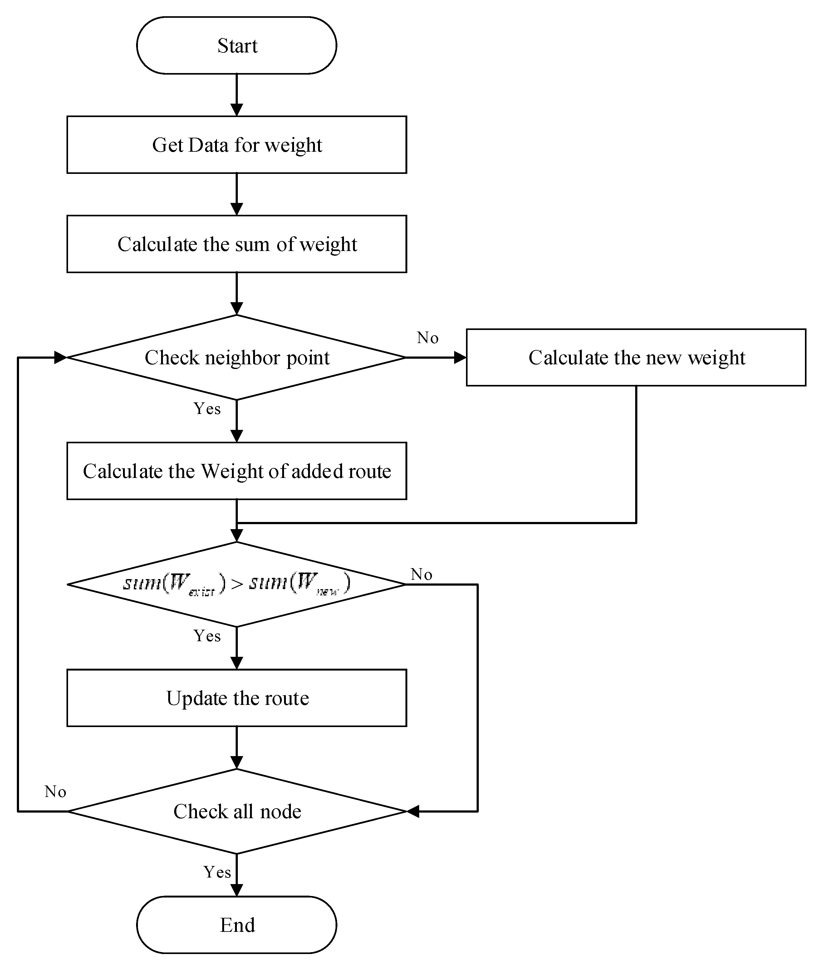
In Figure 1, the points are expressed as nodes and the connected lines between them are assumed to be paths. First, check the weights of each path. Nodes can enter a value; initially it is assumed that all values are infinite. Next, check the weight of the route from the node at the starting point to the neighboring node. Because neighboring nodes currently have infinite values, the identified nodes enter the corresponding weight value. Select the node with the least weight on the neighboring node. Check the weight of the path from the selected node to the neighboring nodes and calculate the weight of the path from neighboring nodes to the value of the neighboring node by adding the weight of the path to the neighboring node with the current node. The value of the current neighboring node and the weight of all paths to the neighboring node are summed and compared with the values of the neighboring nodes. If the value of the neighbor node is smaller, the node with the smallest neighbor value is selected. If the value is smaller than the neighbor node value, the path with the smallest value is selected from the current node. Repeat the process of selecting the node with the smallest weight of the neighboring node, and finally select the path with the smallest weight sum to the destination.

3. Charging Strategy for Charging Stations

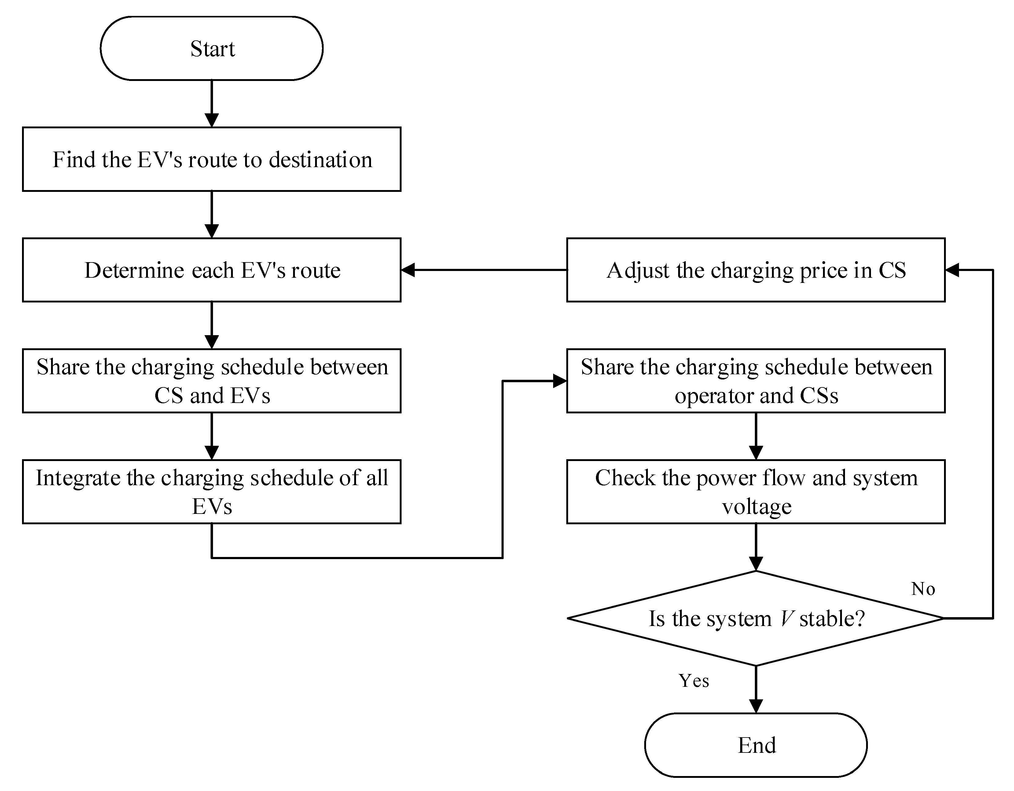
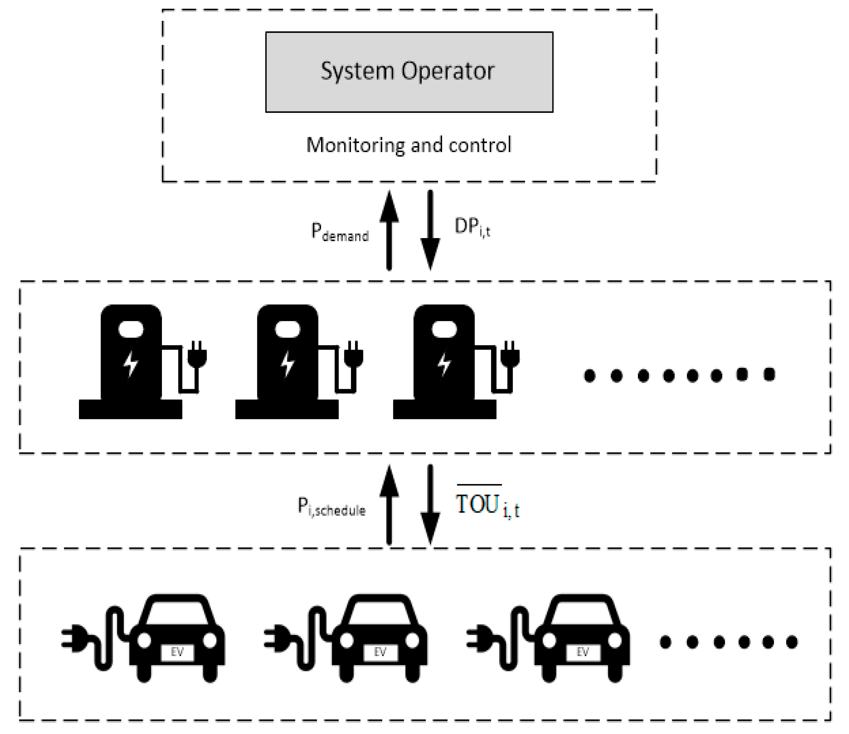
The operator determines the charging price according to the state of the system and sends this information to the CS. The CS then updates the charging price. The inter-layer communication shown in Figure 2 can be described as follows: $P_{demand}$ is the charging schedule of the CS, $D{P}_{i,t}$ is the additional charging price signal of the ith CS at time t, $P_{i,schedule}$ is the charging schedule of the EV, and $\overline{TO{U}_{i,t}}$ is the updated charging price of the ith CS at time t.

The following equations describe the objective function of the EV’s route selection.

$$\arg \min (w_{jk}(i))$$

(1)

$$w_{jk}(i)={\displaystyle \sum _{t=t_{ji}}^{T_{i,t}}(E_{jk}(i)\times \overline{TO{U}_{i,t}})}$$

(2)

$$E_{jk}(i)=S_{jk}(i)/\eta$$

(3)

$$T_{i,t}=\frac{E_{ik}(i)}{P}+t_{ji}$$

(4)

$$\overline{TO{U}_{i,t}}=TO{U}_{i,t}+D{P}_{i,t}$$

(5)

$$0<\overline{TO{U}_{i,t}}$$

(6)

where

• i: charging station;
• j: starting point;
• k: destination point;
• $w_{jk}(i)$: sum of the weights from j to k through charging station i;
• $T_{i,t}$: charging time from t to the charging station i;
• $t_{ji}$: time from j to charging station i;
• $E_{jk}(i)$: amount of energy required to go from j to k through charging station i;
• $E_{ik}(i)$: amount of energy required to go from charging station i to k;
• $S_{jk}(i)$: distance from j to k through charging station i;
• $\eta$: driving power efficiency of EVs (km/kWh); and
• P: rapid charging power.

The EV uses Dijkstra’s algorithm to determine the route with the minimum cost, as shown in Equation (1). Equations (2)–(6) are constraints. Equation (2) is a measure of the weight value of each route calculated by multiplying the energy required for driving by the charge price. Equation (3) is the required energy calculation for the driving distance considering charging station i. Equation (4) is a formula for the time spent charging at charging station i. Since the charging power of the CS is a constant, it was used to check the charging time of the EV arriving at the charging station and apply it to the charging schedule. Equations (5) and (6) are constraints on dynamic prices as the dynamic pricing signal. The dynamic pricing signal should be added or subtracted to the existing TOU (Time-of-Use) price, and the reflected price should be positive.

Figure 3 shows the operating algorithm of the system operator. First, EV driving data is developed as a probability model based on actual highway data. These data are the number of vehicles that pass-through toll gates on inter-hourly highways and are modelled with the probability that vehicles have passed during each time period. The route will be selected considering the price information for charging the battery, driving distance of the vehicle, normal speed for the road on which it is driven, starting time, and destination. The route selection algorithm is shown in Equation (1) and is performed by individual EVs. The cost of charging the battery will act as a weight in the route selection algorithm, and the charging price will determine the route that can be driven at the minimum cost. It is assumed that when an EV user selects a driving route, it passes through a charging station once. Charging stations that receive the time the vehicle arrives at the charging station incorporate the information to schedule the charging demand. The charging station shares the charging schedule with the system operator. The price information of the reflected charging station shares information with the vehicle in real time, and the vehicle that sets the driving route sets the route with the updated price information.

The CS transmits the schedule obtained from the electric vehicle to the system operator. Using the Gauss–Seidel method, the system operator calculates the power flow of the system based on the schedule obtained from the CS [10]. By analyzing power flow with the schedule, the voltage can be predicted in advance. A voltage threshold value is set according to the system conditions. When the voltage exceeds the threshold value, a dynamic pricing signal is sent. The dynamic pricing signal is calculated using Equation (7). When the system operator sends the price signal to the CS, the CS immediately responds to this signal and sends the information to the EVs. The equation guiding the above interaction is as follows:

$$D{P}_{i,t}=(\begin{array}{c}\alpha (V_{DL}-V_{i,t})\times C,V_{i,t}<0.95\\ \alpha (V_{UL}-V_{i,t})\times C,V_{i,t}>1.05\end{array}$$

(7)

where

• $\alpha$: weight for dynamic pricing;
• $V_{DL}$: lower limit voltage value;
• $V_{UL}$: upper limit voltage value;
• $V_{i,t}$: voltage of bus i at time t; and
• $C$: instantaneous voltage drops loss cost.

It is difficult to obtain accurate statistical data of the cost due to instantaneous voltage drops, so they are estimated using statistical data of the cost [11,12]. In a typical power system, the voltage range is from 0.95 to 1.05 p.u., so the maximum and minimum voltages are set to 1.05 and 0.95, respectively. Figure 3 shows a flow chart of the overall system.

4. Simulation Results

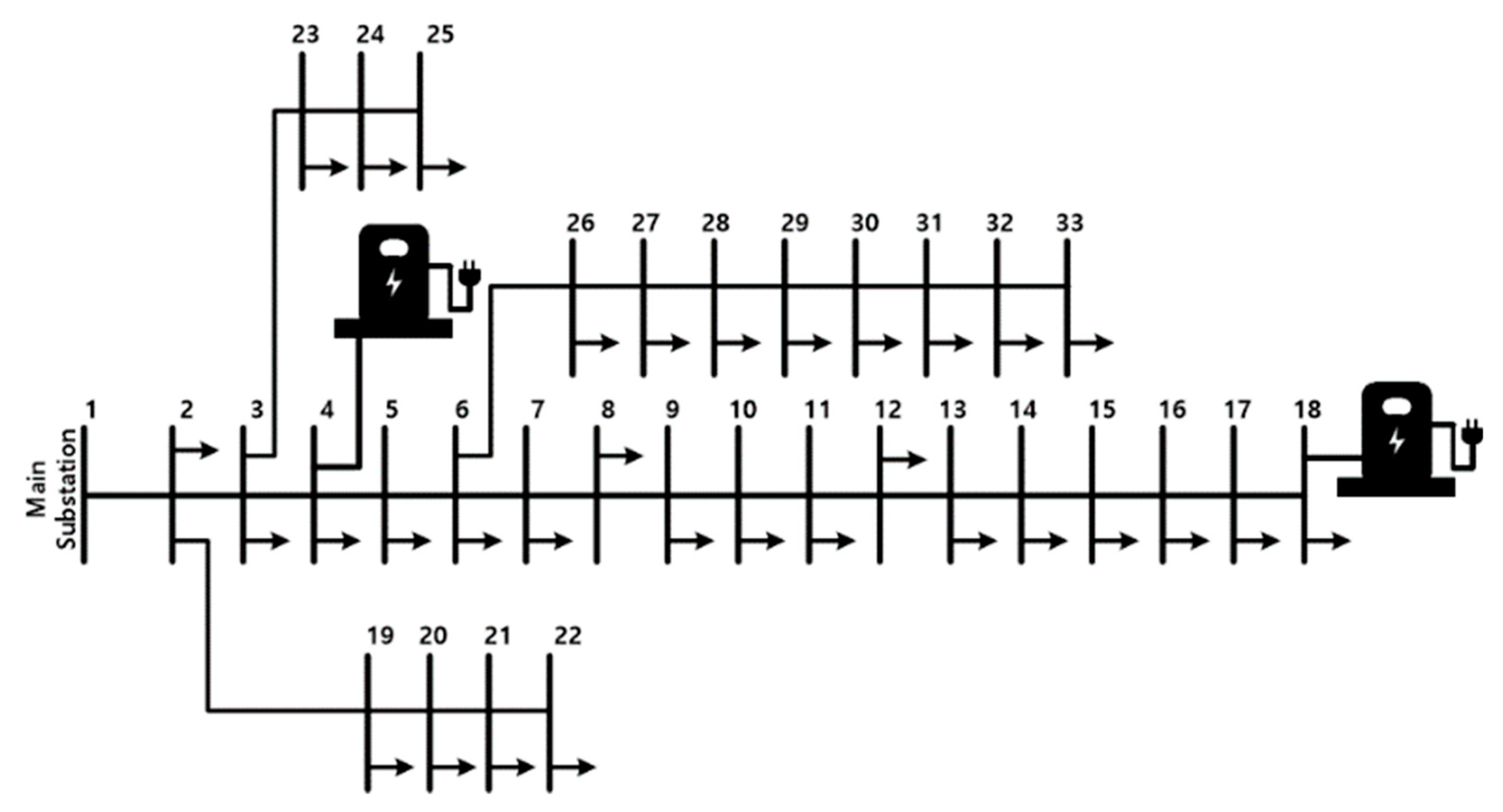
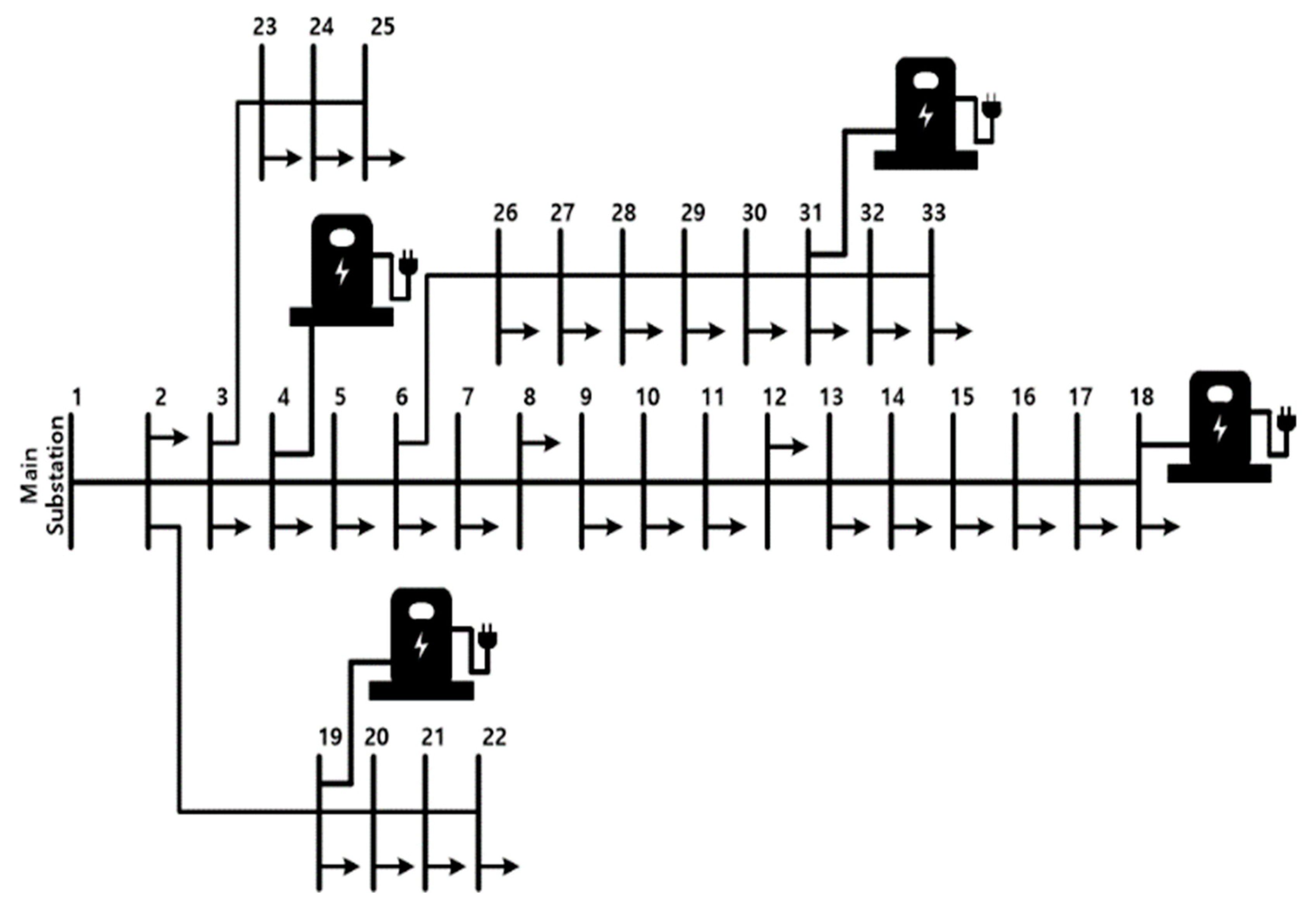
For the simulation, the system was constructed with reference to the IEEE-33 test bus [13]. As shown in Figure 4, the voltage regulation was confirmed using the IEEE-33 test bus, with the CSs arranged according to the scenario in the IEEE 33 bus node. For the EV parameters, the size of the battery was set to 30 kWh, and the energy consumption to 5 km/kWh, following Nissan’s Leaf. The number of vehicles from the departure point to the destination were applied to the simulation. And

Table 1. The simulation scenario with dynamic pricing.

Scenario	Case 1	Case 2	Case 3	Case 4
Dynamic Pricing	X	O	X	O
Number of Charging Stations	2	2	4	4
Number of Starting Points	1	1	2	2

also shows scenarios for simulation analysis.

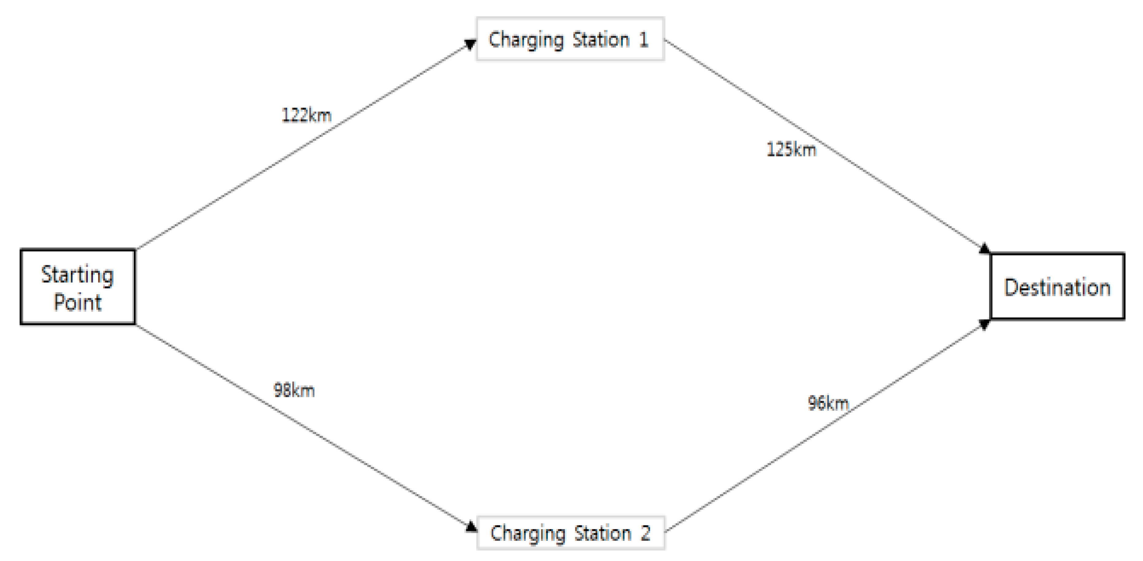
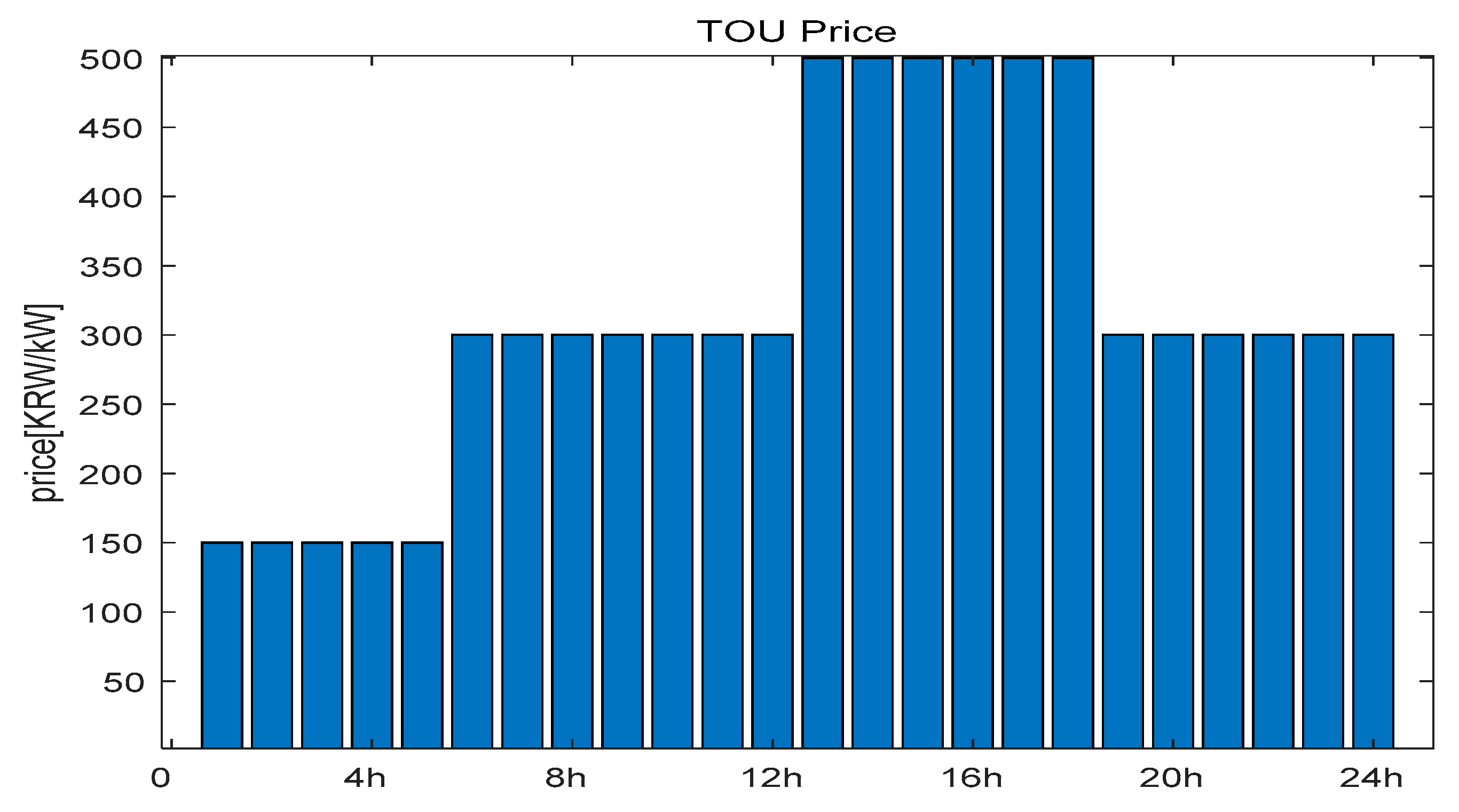
Case 1 is the base scenario for comparing simulation results. Figure 5 represents a route containing two charging stations to a destination. Figure 6 shows the TOU information used in the simulation. The CS is simulated with the TOU price. To verify the proposed control strategy, the basic system consisted of two CSs, one destination point, and one starting point. CS 1 was located at node 4 and CS 2 was located at node 18, as shown in Figure 4. In this paper, the schedule of the CS and the route were confirmed for the EV that was taken when the fixed price plan was applied in the basic system. In addition, when price fluctuations due to dynamic pricing occur, they were compared with the schedule of the CS and its route. The voltage regulation of the vehicle CS changed by price fluctuations through dynamic pricing was confirmed. It was also confirmed that the route changed.

4.1. Case 1

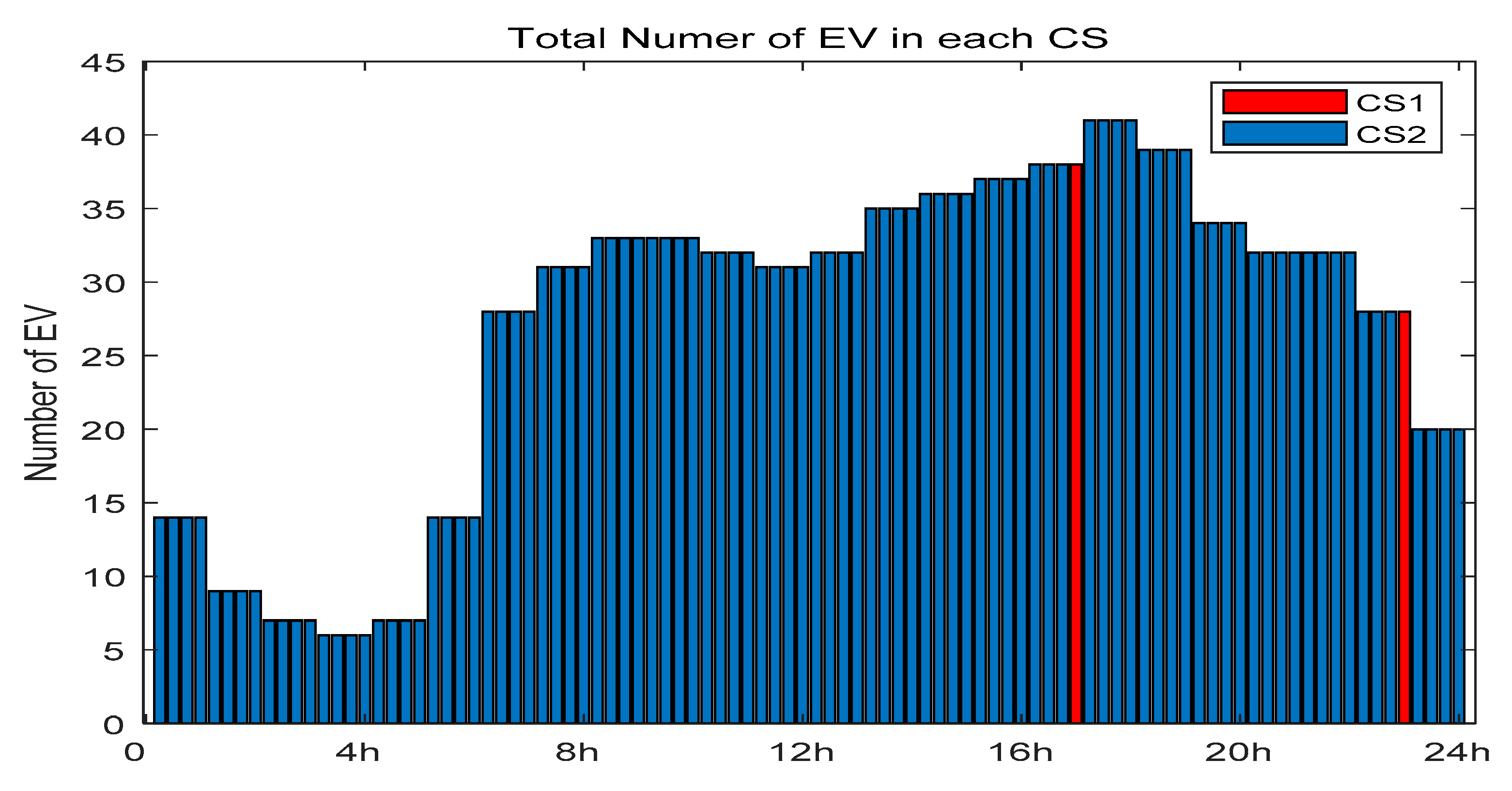
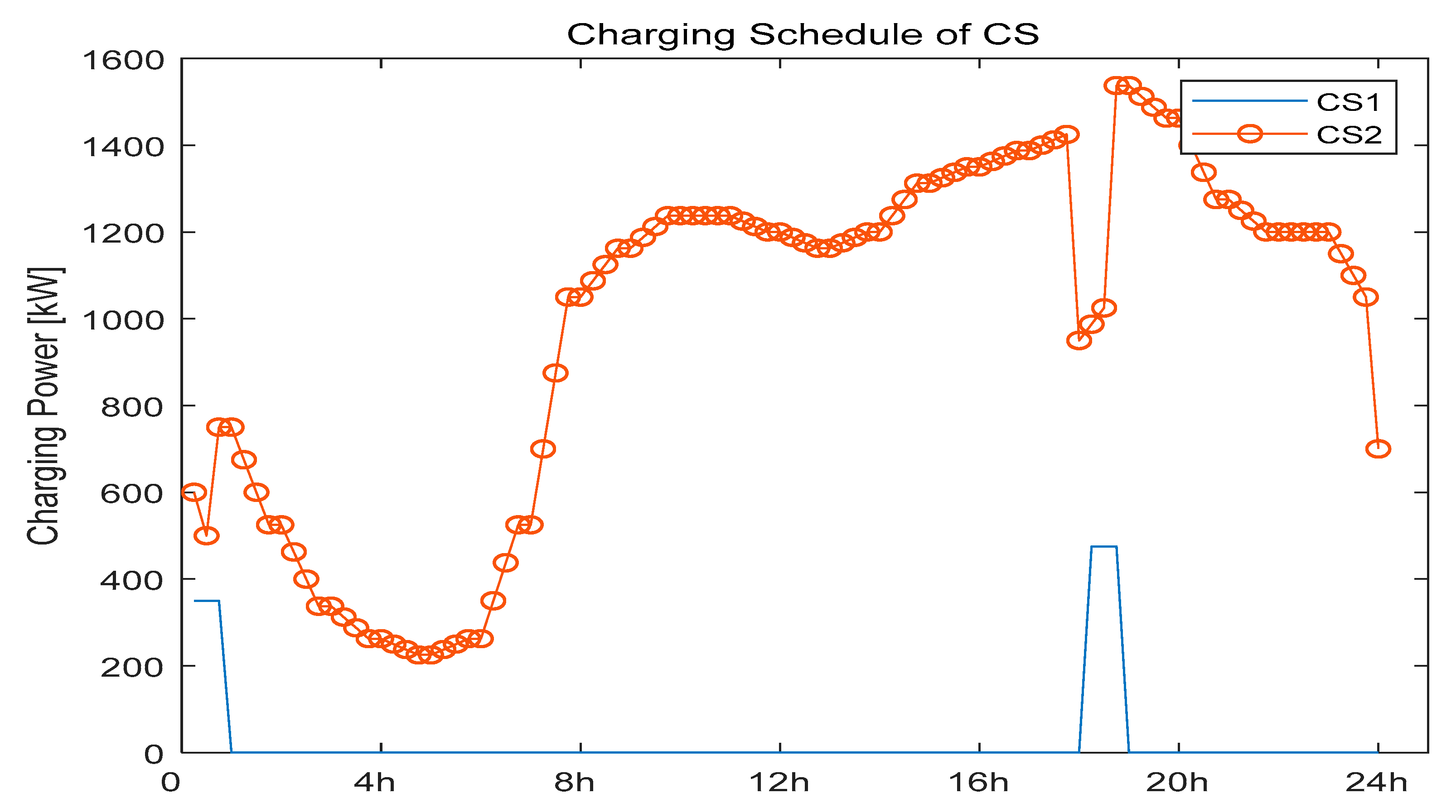
When operating a CS with a fixed pricing system without dynamic pricing, the EV can be confirmed as a route with CS 2, as shown in Figure 7. When calculating the minimum cost route, the EV considers the arrival time, distance, and the TOU price at arrival time. EVs were set up mostly at CS 2, as can be seen in Figure 8. Most EVs were concentrated at CS 2, which consumed up to 1.5 MW per day. The number of EVs was relatively lower during the early hours for CS 2 than during the day, leading to lower power consumption for those hours. The peak power demand occurred from 7:00 to 8:00 p.m. In the afternoon, the power demand for CS 2 decreased and that of the CS 1 increased. This result shows that the TOU price fluctuated when the EV determined the route. If the EV was set to go through CS 2, it was charged when the TOU price was KRW 500 per kW. If the EV was set to go through EV 1, when the TOU charge was KRW 300 per kW, it took the route going through CS 1. For this reason, in the afternoon and at dawn, the EV set CS 1 as its route. In Figure 9, the time of day and afternoon are checked.

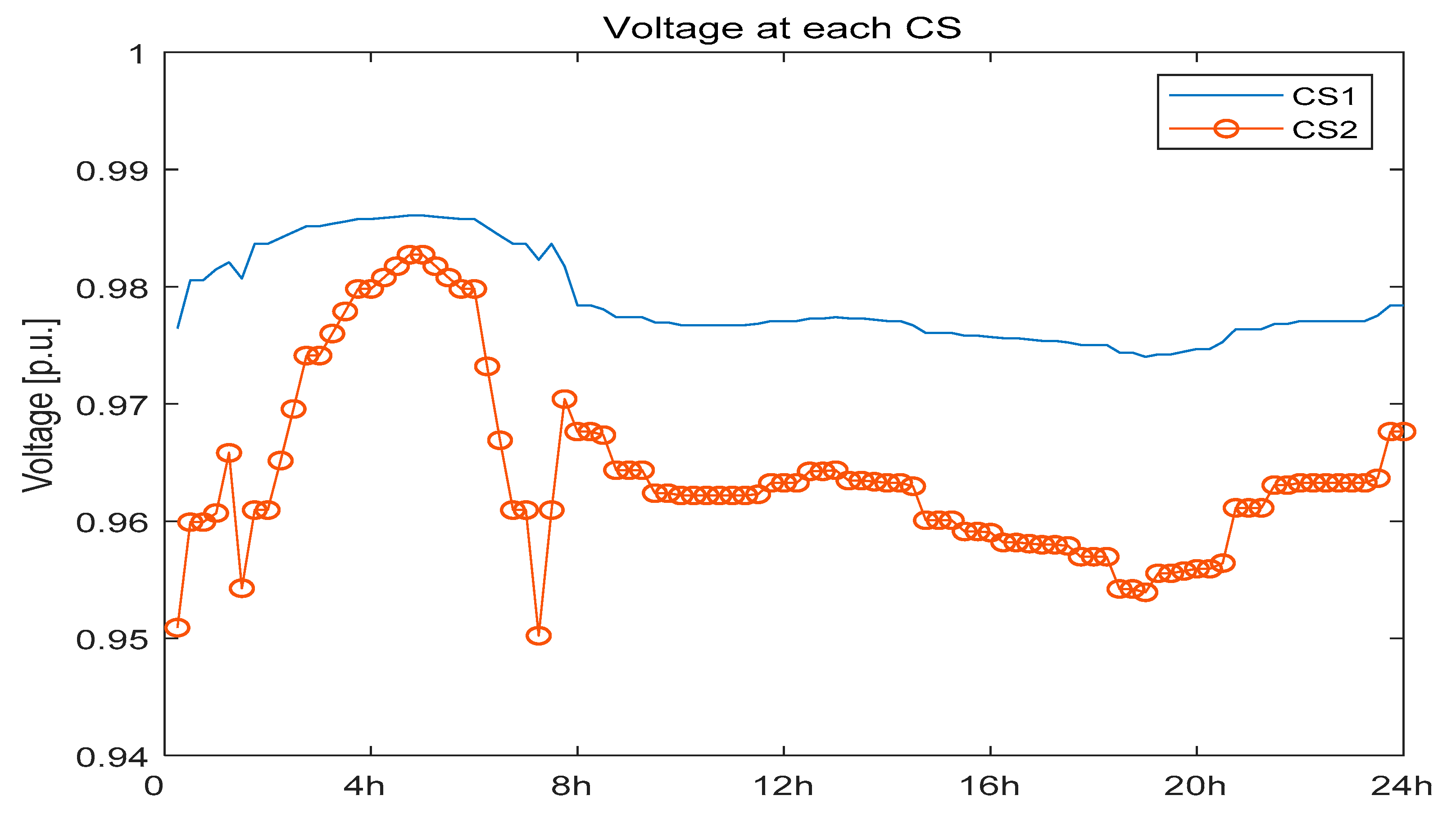
The voltage decreased as the charge energy of the CSs became larger while the vehicle travelled on the determined route of the EV. Figure 9 shows that the voltage changed according to the charging schedule of the CS. The charging schedule of CS 2 confirms that the voltage fell in accordance with the charging schedule (the voltage dropped to a maximum of about 0.93 p.u.). Conversely, when the voltage of CS 1 (that did not include the route of the EV) was checked, the voltage dropped to about 0.97 p.u. In general, the graph of the voltage varies according to the charging schedule of the CS.

Table 2. Summary of simulation results in Case 1.

Charging Station (CS)	CS 1	CS 2
Maximum Charging Power [kW]	457	1537.5
Minimum Charging Power [kW]	0	225
Highest Charging Price [KRW/kW]	500	500
Lowest Charging Price [KRW/kW]	150	150
Lowest Voltage [p.u.]	0.9724	0.9255

shows a summary of the simulation results for each charging station.

4.2. Case 2

In Case 2, the results were obtained when the base system applied price fluctuations rather than fixed price plans. Figure 10 shows the CS selected by the route of the EV when the price was changed by applying dynamic pricing. Compared to Figure 7, there is a clear difference. Most of the consequences of the concentration on CS 2 were alleviated, and the electric vehicle could be charged at CS 1.

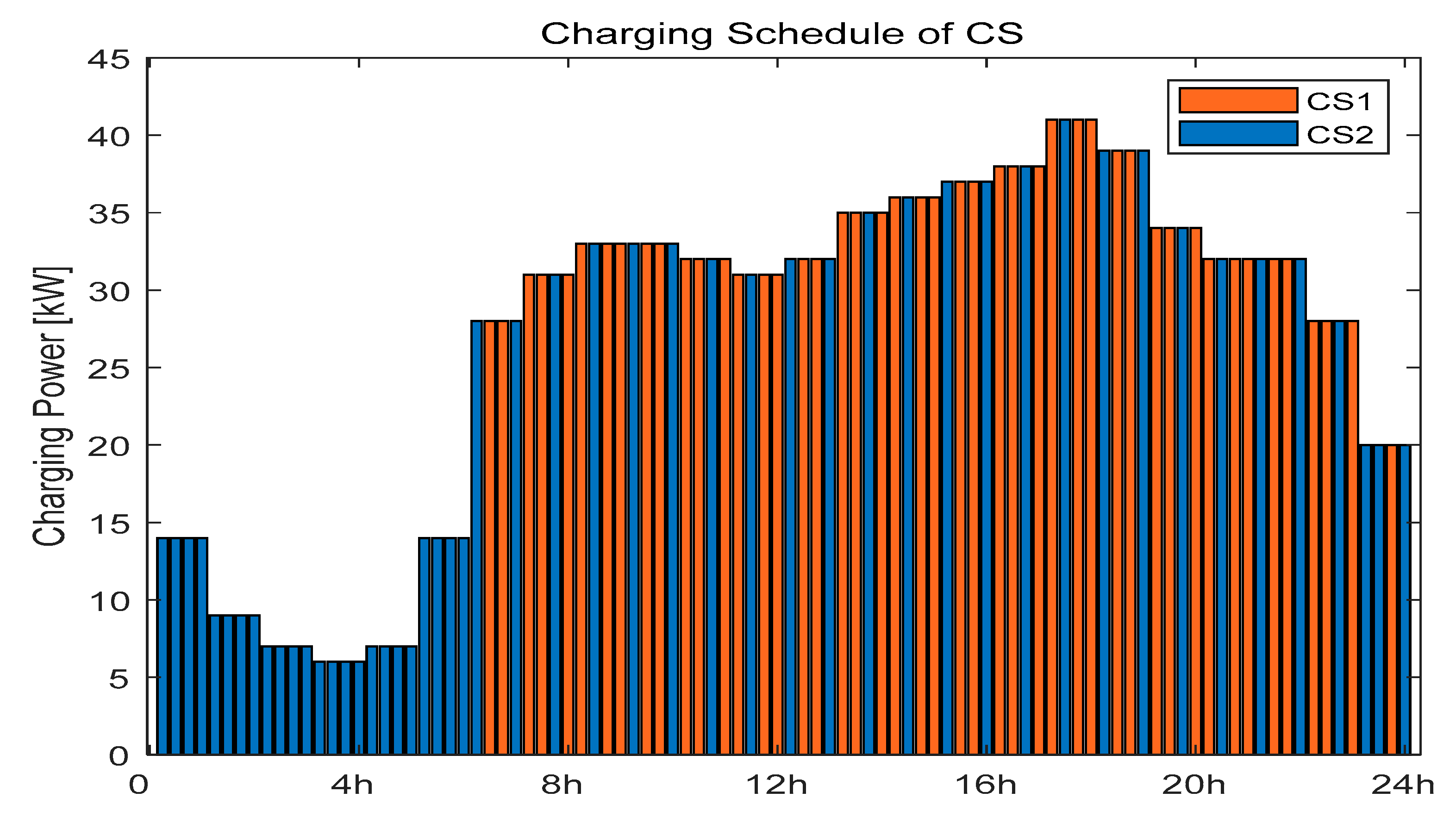
Figure 10 shows the charging schedule for the CS, with different results. Previously, as there was concentration on CS 2, its charging schedule showed a high demand for power. However, as a result of applying the control strategy, the charging energy demand for CS 1 was higher than that for CS 2 in the afternoon. As the price fluctuated due to dynamic pricing, the route of the EV that was about to go to CS 2 changed so that it passed through CS 1. During the dawn hours from 1:00 to 6:00 a.m., the number of EVs was relatively small, so the EV route was designated as EV 2. However, as the number of EVs increased from the afternoon on, the system operator confirmed the charging schedule of the CS and sent the dynamic pricing signal to the CSs according to the voltage. If the voltage of the CS was lowered to 0.95 p.u., the system operator reset each EV’s route with the price signal to the CS according this voltage. Therefore, the EV reset the price of the CS and recalibrated the route. The change in the route of the EV helped to distribute the charging energy between CS 1 and 2 appropriately.

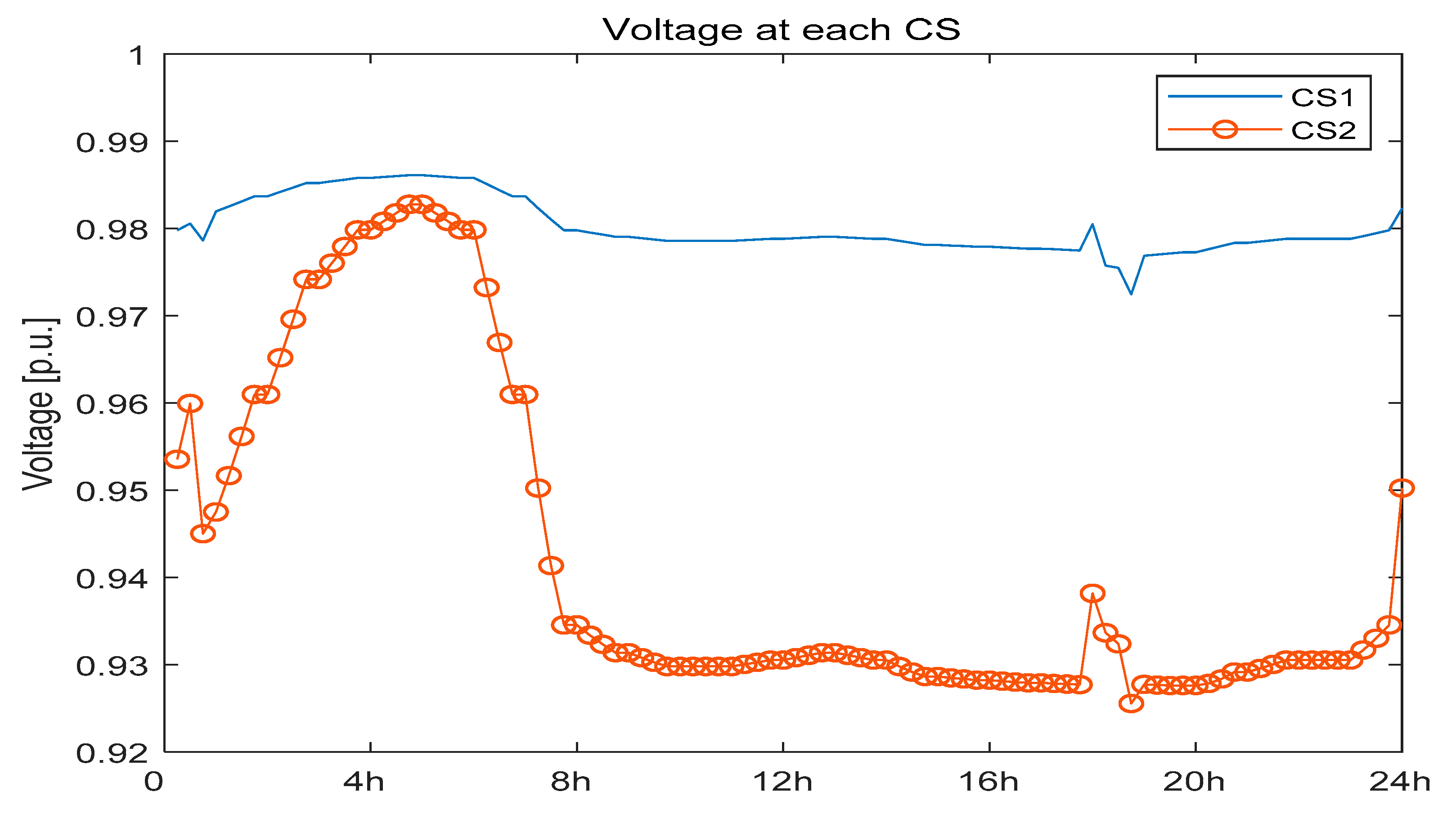
Figure 11 is a graph showing the appropriately distributed voltage of the CSs. As the demand for charging energy was distributed, so was the voltage of the CSs. The voltage for CS 2 did not fall below 0.95 p.u. The voltage of CS 1 was lowered, but it did not drop below 0.95 p.u.

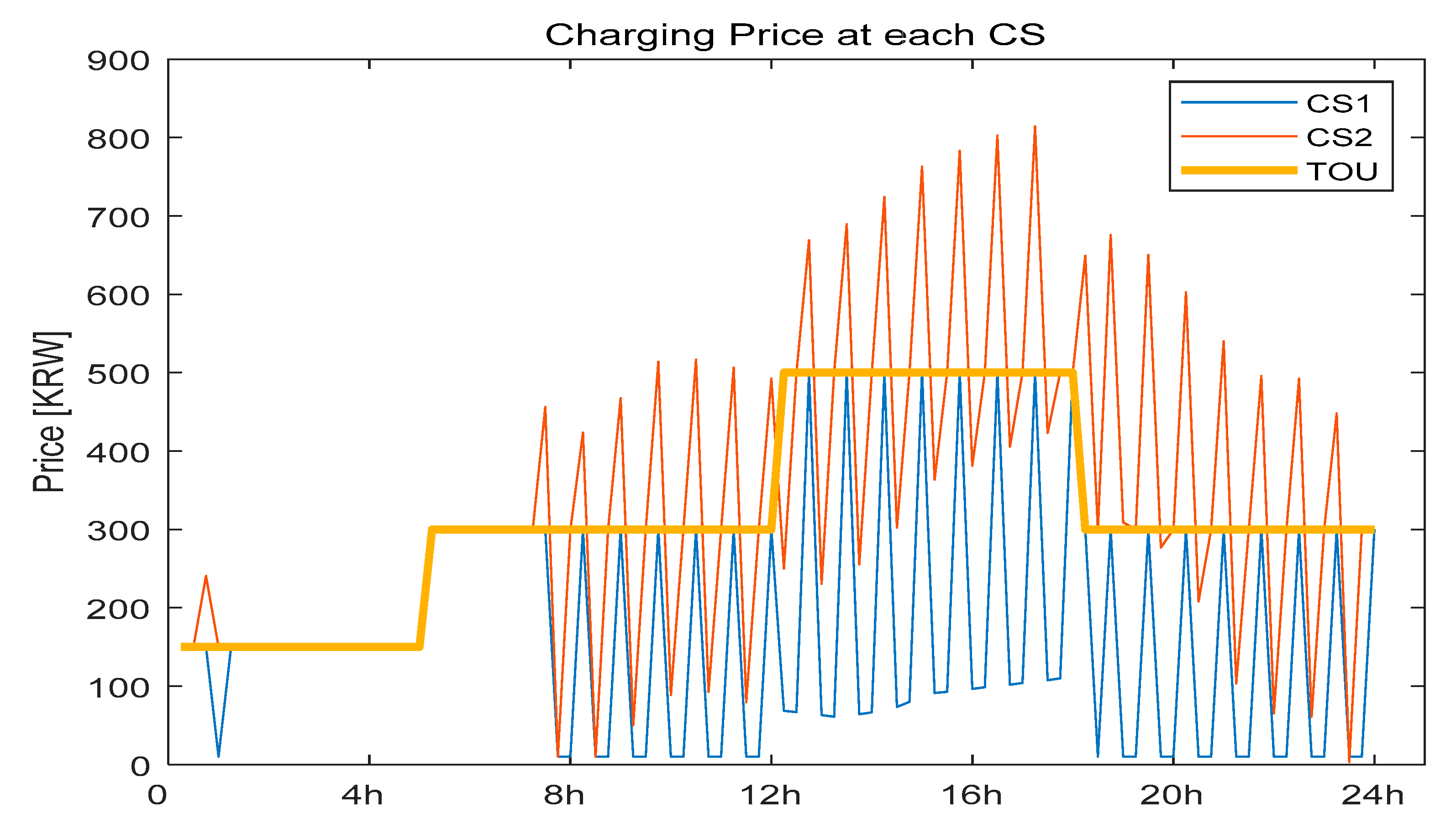
Figure 12 shows the charging price for CS 1 and 2. From the system operator’s point of view, if the voltage became lower than 0.95 p.u., the charging schedule of the CS was checked and It can provide a price change in a dynamic pricing, depending on the control strategy of the CS. Unlike the conventional TOU price, the prices of CS 1 and 2 varied in real time. In general, the price of CS 2 was higher than that of both CS 1 and the TOU price. The reason for this is that the system operator confirmed the voltage and could predict that the voltage of CS 2 would be lower than the set value, so the charging price of CS 2 was set high. The price of CS 1 fluctuated and became less than the TOU price at a time when EVs charge up. This change caused the EV to charge at CS 1 rather than at CS 2, because the EV sets the route according to the charging price at the route setup time. To designate the EV route as CS 1, the charging rate was under about KRW 100, and in the opposite situation, the charging rate of CS 2 was about KRW 800.

Table 3. Summary of simulation results in Case 2.

Charging Station (CS)	CS 1	CS 2
Maximum Charging Power [kW]	1025	700
Minimum Charging Power [kW]	0	225
Highest Charging Price [KRW/kW]	500	814
Lowest Charging Price [KRW/kW]	10	10
Lowest Voltage [p.u.]	0.974	0.9502

shows a summary of the simulation results.

4.3. Case 3

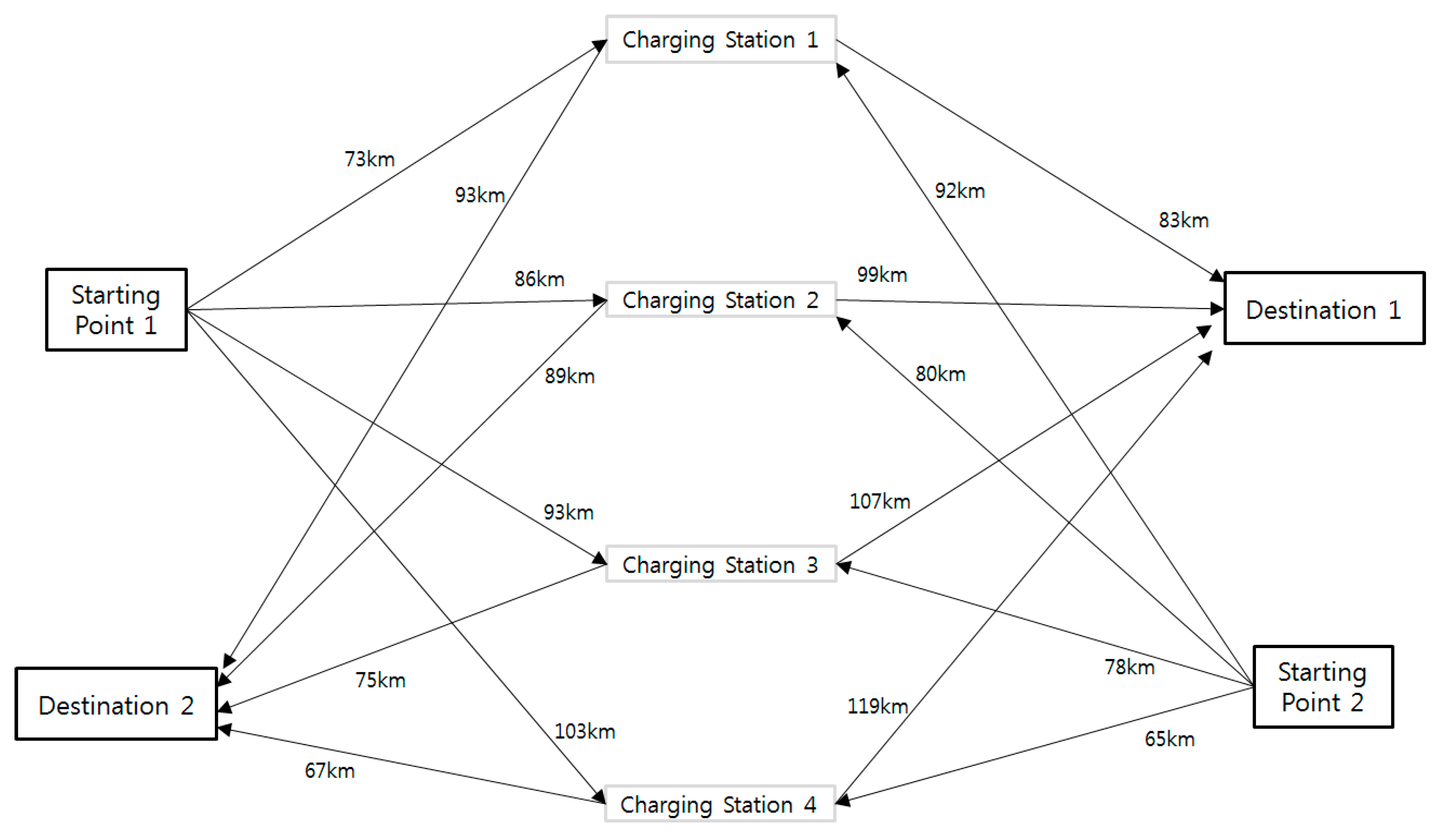
In Case 3, the four CSs constructed in the multiple systems were located, as shown in Figure 13. CS 1 was configured at node 18, CS 2 at node 31, CS 3 at node 4, and CS 4 at node 19.

Figure 13 shows the distance between the starting point and the CSs, and the distance between the CSs to the destination point. The time taken for each point was set to a random value proportional to the distance. When operating an CS with a TOU price without dynamic pricing, it is seen that EVs were driven into two CSs, as shown in Figure 14. Because the distances through CS 1 and CS 4 are short, the EVs gathered into CS 1 and CS 4 and the charging schedule of the CS could be confirmed. When the EV considered the cost when setting the route, starting point 1 determined the route to CS 1, while starting point 2 determined the route to CS 4 in most cases. As a result, the charging schedule for the CS was set as shown in Figure 14. Most EVs were concentrated at CS 1 and CS 4, which consumed up to 1.3 MW per day. During the early hours, the number of vehicles was relatively lower for CS 1 and 4 than during the daytime, implying that they consumed less power during the early hours, while peak power demand occurred around 7:00 to 8:00 p.m.

There was a slight difference in the charging schedule of the CSs for CS 1 and CS 4. This difference was due to the stochastic model. In the afternoon, the power demand at CS 1 and CS 4 decreased, while the demand at CS 2 and CS 3 increased. This is in consideration of the change in the TOU price when the EV arrived at the CS. For example, at first, when the EV sets the route, it goes from starting point 1 through CS 1, and from starting point 2 through CS 4 because of the short travel distance. At this time, the arrival time at the CS changed, so the TOU price was charged at KRW 500/W and KRW 300/kW, according to the arrival time. Considering the TOU price variance, the EV decided on a route that could be changed at a minimum cost, and the power demand for CS 2 and CS 3 increased according to the charging schedule. Figure 15 shows the results from 0:00 to 1:00 a.m. and from 6:00 to 7:00 p.m.

4.4. Case 4

Case 4 shows the results when dynamic price was applied to the CSs. As shown in Figure 14, in Case 3 with no dynamic price, the EV was driven a short distance to CS 1 and CS 4. Therefore, the voltage in CS 1 dropped to 0.9266 p.u., as shown in

Table 4. Summary of simulation results for Case 3.

Charging Station (CS)	CS 1	CS 2	CS 3	CS 4
Maximum Charging Power [kW]	1087.5	625	650	1300
Minimum Charging Power [kW]	0	0	0	150
Highest Charging Price [KRW/kW]	500	500	500	500
Lowest Charging Price [KRW/kW]	150	150	150	150
Lowest Voltage [p.u.]	0.9266	0.9459	0.9678	0.9932

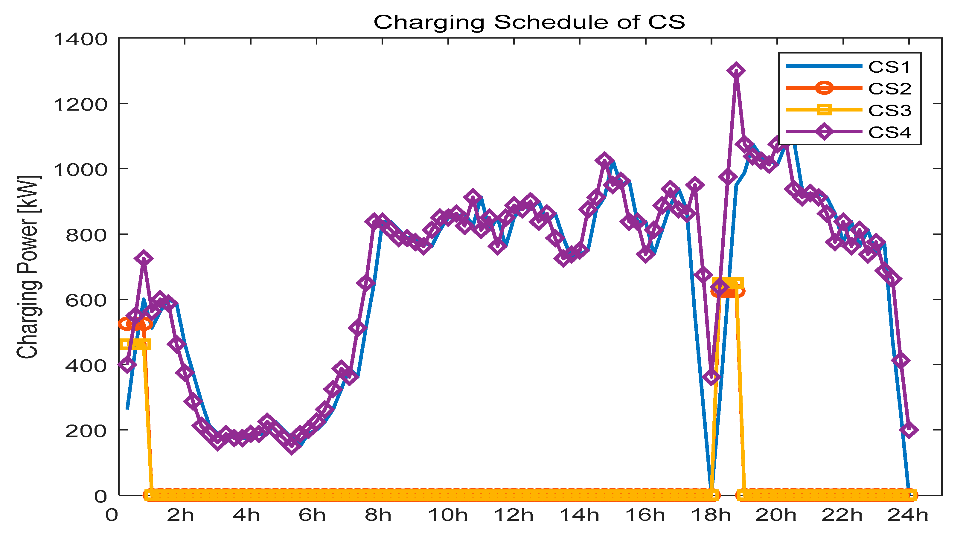
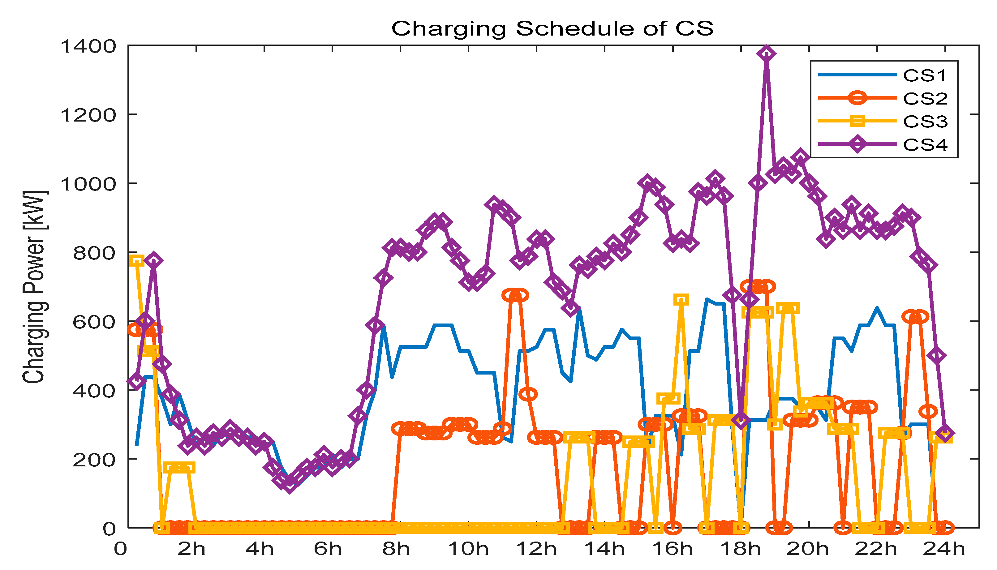
. The graph in Figure 16 shows which CS was selected by the route of the EV when the price was changed by applying dynamic pricing. The concentration at CS 1 and CS 4 was alleviated, and EVs were also charged at CS 2 and CS 3. The graphs in Figure 16 show the charging schedules for CSs. As a result of applying the control strategy, a demand for power was suddenly generated at CS 2 and CS 3 after 8:00 a.m. Due to dynamic pricing, the EV’s route to CS 1 and CS 4 was changed to CS 2 and CS 3. Thus, unlike in Case 3, the voltage adjustment was performed as charging demand was distributed. 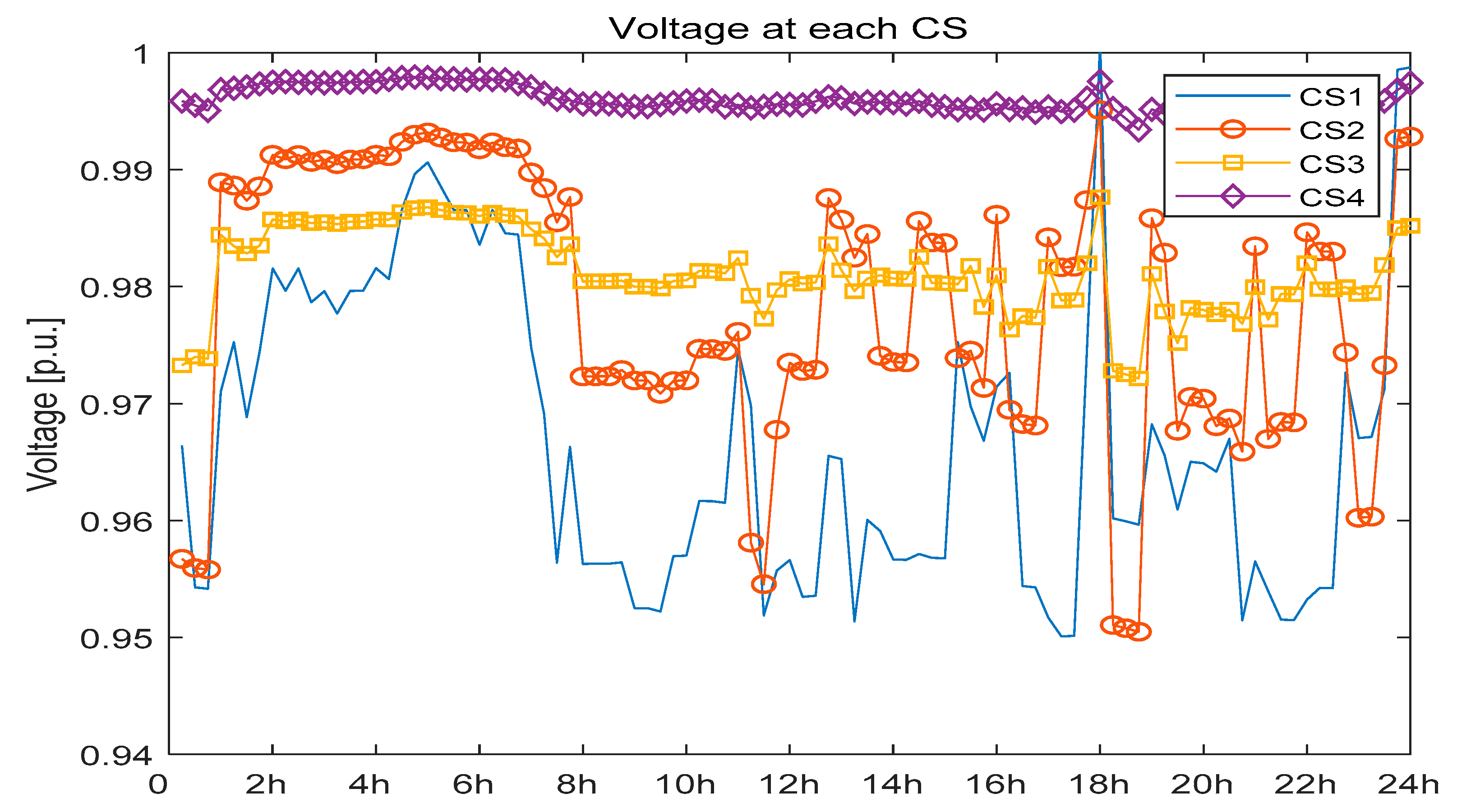In Figure 17 the voltage at CS 1 (blue line) does not drop to less than 0.95. Through dynamic pricing, the system operator ensured that the voltage at the CS did not exceed 0.95 p.u. Change in price led to changes in the route of the EV to properly distribute the energy demand of the CSs.

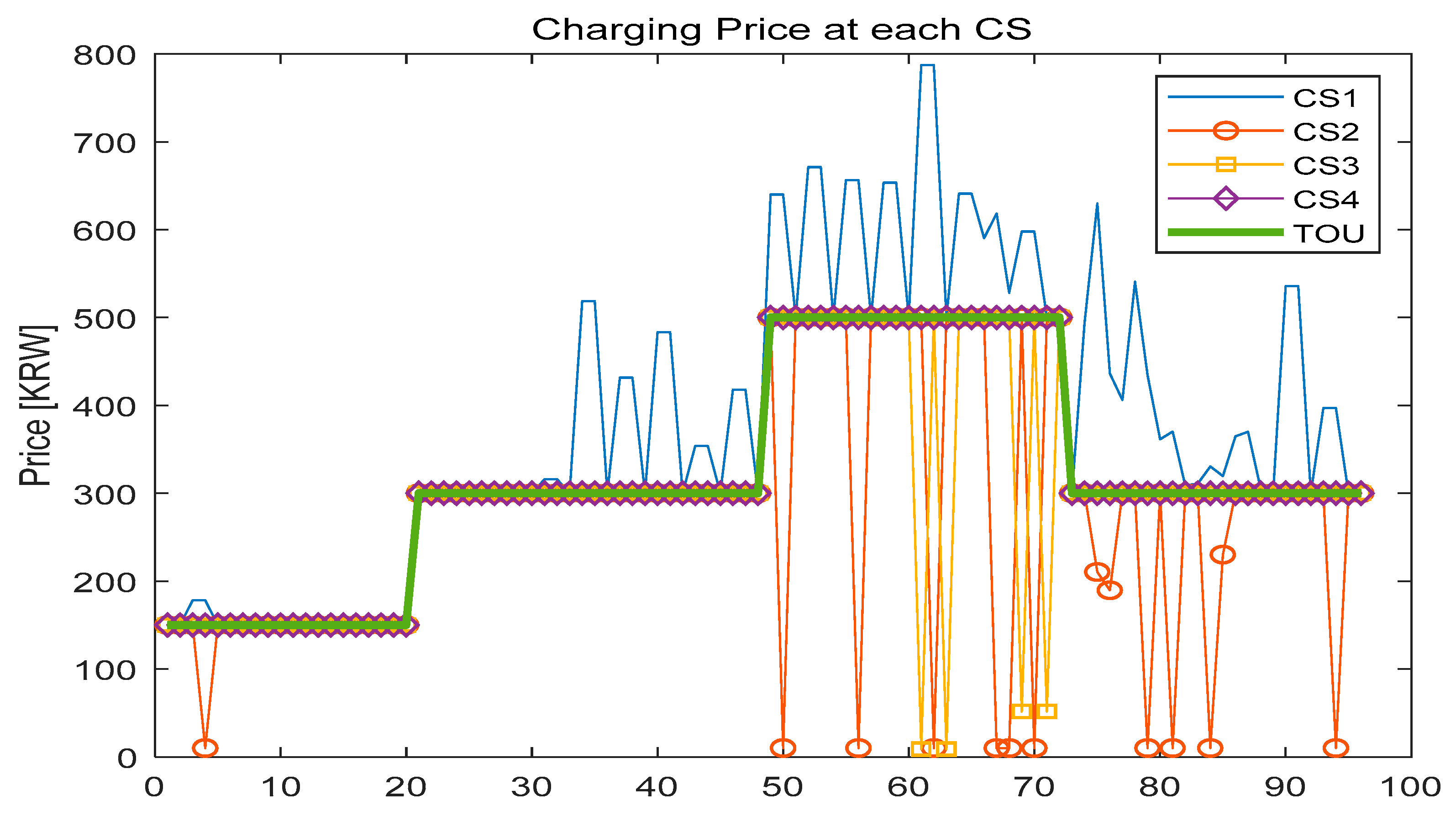
Figure 18 shows a charging price graph for voltage regulation. The system operator checked the charging schedules of all CSs in advance and determined that voltage regulation was necessary. Thus, a dynamic price graph like Figure 18 was derived to distribute the charging demand. To derive the path for EV charging in CS 2 and CS 3, the price charged was lowered to less than KRW 100. In contrast, to suppress charging prices CS 1 rose to around KRW 790. The grid operator first checked the voltage in real time, then adjusted the price to lower the charge demand of the CS. Reflecting the adjusted price, the EV selected a driving route again. Therefore, once the price was changed, the driving route of the EV is changed, and the price stabilized again because the system operator confirmed that the charging demand was distributed. Unlike the earlier case 3, the voltage cannot determine where to fall below 0.95 p.u. This is because CS 2 and CS 3 lowered the charging price to induce charging of electric vehicles, which can be seen in

Table 5. Summary of Simulation Results in Case 4.

Charging Station (CS)	CS 1	CS 2	CS 3	CS 4
Maximum Charging Power [kW]	662.5	700	775	1375
Minimum Charging Power [kW]	0	0	0	125
Highest Charging Price [KRW/kW]	787	500	500	500
Lowest Charging Price [KRW/kW]	150	10	10	150
Lowest Voltage [p.u.]	0.9501	0.9505	0.9721	0.9934

.

5. Conclusions

In this paper, a method was proposed for distributing power demand between CSs to improve the system through route selection for EVs in a grid using Dijkstra’s algorithm and dynamic pricing. The EV considers the distance from the CS using the price information, as well as the time it takes to get to the destination, depending on traffic conditions. The EV uses Dijkstra’s algorithm to find the minimum charging cost route. The EV transmits information on charging time and size of the charging energy to the CS on the route of the EV. At the CS, the charging schedule of the CS is integrated by compiling the information from the EVs. The system operator compiles the charging schedule for the CSs and determines the voltage of the system based on the charging schedule. The operator judges the voltage and detects risk factors in the system in advance, changing the charging price of the CS in real time. The changed price signal is sent to each CS, and is set so that the EV reflects the new price, while information about the route is updated in the charging schedule of the CS. The configuration for the system and verification of the proposed algorithm was performed using MATLAB.

The system operator predicts the unstable factors of the system by using a schedule that considers the path of the EV. Operational costs can be reduced because the risk can be predicted in advance, and EV users can benefit economically from dynamic pricing. In future research it will be necessary to construct a stochastic modelling of vehicles using Big-Data and to conduct studies considering sudden events. The system operator should know the correlation between the price signal and the operating cost. The more EVs and CSs, the more advantages can be obtained from stable operation of the grid through dynamic pricing.

References

- Bilh, A.; Naik, K.; El-Shatshat, R. A Novel Online Charging Algorithm for Electric Vehicles Under Stochastic Net-Load. IEEE Trans. Smart Grid 2018, 9, 1787–1799. [Google Scholar] [CrossRef]
- Hou, K.; Xu, X.; Jia, H.; Yu, X.; Jiang, T.; Zhang, K.; Shu, B. A Reliability Assessment Approach for Integrated Transportation and Electrical Power Systems Incorporating Electric Vehicles. IEEE Trans. Smart Grid 2018, 9, 88–100. [Google Scholar] [CrossRef]
- Tang, D.; Wang, P. Probabilistic Modeling of Nodal Charging Demand Based on Spatial-Temporal Dynamics of Moving Electric Vehicles. IEEE Trans. Smart Grid. 2016, 7, 627–636. [Google Scholar] [CrossRef]
- Del Razo, V.; Jacobsen, H.A. Smart Charging Schedules for Highway Travel with Electric Vehicles. IEEE Trans. Transp. Electrif. 2016, 2, 160–173. [Google Scholar] [CrossRef]
- Zhou, Y.; Yau, D.K.; You, P.; Cheng, P. Optimal-Cost Scheduling of Electrical Vehicle Charging Under Uncertainty. IEEE Trans. Smart Grid 2018, 9, 4547–4554. [Google Scholar] [CrossRef]
- Gusrialdi, A.; Qu, Z.; Simaan, M.A. Distributed Scheduling and Cooperative Control for Charging of Electric Vehicles at Highway Service Stations. IEEE Trans. Intell. Transp. Syst. 2017, 18, 2713–2727. [Google Scholar] [CrossRef]
- Lu, J.; Dong, C. Research of shortest path algorithm based on the data structure. In Proceedings of the 2012 IEEE International Conference on Computer Science and Automation Engineering, Beijing, China, 22–24 June 2012; pp. 108–110. [Google Scholar]
- Mena, F.M.; Ucan, R.H.; Cetina, V.U.; Ramirez, F.M. Web service composition using the bidirectional Dijkstra algorithm. IEEE Lat. Am. Trans. 2016, 14, 2522–2528. [Google Scholar] [CrossRef]
- Swathika, O.G.; Hemamalini, S. Prims-Aided Dijkstra Algorithm for Adaptive Protection in Microgrids. IEEE J. Emerg. Sel. Top. Power Electron. 2016, 4, 1279–1286. [Google Scholar] [CrossRef]
- Saadat, H. Power System Analysis, 2nd ed.; McGraw-Hill Primis Custom Publishing: New York, NY, USA, 2002; pp. 190–219. [Google Scholar]
- Lee, K.; Han, J.H.; Jang, G.; Park, C.H. Method to select optimal device for mitigating voltage sag based on voltage sag assessment. Trans. Korean Inst. Electr. Eng. 2015, 64, 29–34. [Google Scholar] [CrossRef]
- Han, J.H.; Jang, G.; Park, C.H. A Study of Economic Assessment of Voltage Sag Mitigation Devices. In Proceedings of the 43th KIEE Summer Conference, Jeongseon-gun, Korea, 18–22 July 2012; pp. 60–61. [Google Scholar]
- Aman, M.M.; Jasmon, G.B.; Bakar, A.H.A.; Mokhlis, H. Optimum network reconfiguration based on maximization of system loadability using continuation power flow theorem. International Journal of Electr. Power Energy Syst. 2014, 54, 123–133. [Google Scholar] [CrossRef]
Figure 1.
Flowchart of Dijkstra’s algorithm.
Figure 2.
Operation scheme of the system.
Figure 3.
Flowchart of the system operator.
Figure 4.
Modified IEEE 33 test bus system with two CSs.
Figure 5.
Route from starting point to destination.
Figure 7.
EV’s CS selection rate in Case 1.
Figure 8.
Charging schedule of CSs in Case 1.
Figure 9.
Voltage of CSs in Case 1.
Figure 10.
EV’s CS selection rate in Case 2.
Figure 11.
Voltage of CSs in Case 2.
Figure 12.
Charging price of CSs in Case 2.
Figure 13.
Modified IEEE 33 test bus system with four CSs.
Figure 14.
Figure 15.
Charging schedules of CSs in Case 3.
Figure 16.
Charging schedule of CSs in Case 4.
Figure 17.
Voltage of CSs in Case 4.
Figure 18.
Charging price of CSs in Case 4.