Power Transformer’s Electrostatic Ring Optimization Based on ANSYS Parametric Design Language and Response Surface Methodology

Abstract

In this paper, in view of the low efficiency of the traditional finite element method (FEM), which has been widely used in the insulation design of power transformers, the response surface methodology (RSM) is proposed to optimize the insulation structure of a power transformer electrostatic ring. Firstly, the power transformer model was built using the ANSYS parametric design language (APDL) to realize the automatic pre-processing of numerical calculation. Then with the objective of reducing the maximum electric field intensity, the Taguchi method was used to select the parameters that have a greater impact on the maximum electric field intensity, by which the subsequent optimization process could be effectively simplified. The test points were constructed by the central composite design (CCD) and a response surface model was established by the mutual calls of MATLAB and ANSYS. Finally, the variance analysis, diagnostic analysis, and significance test of regression were carried out to obtain the final response surface model. By comparing the result of RSM with that of FEM, we can find that the results obtained by the two methods are consistent and the maximum electric field strength is obviously reduced. The RSM is more systematic and convincing, which improves the optimization efficiency and provides a reliable and fast way for the optimization of power transformers.

1. Introduction

As the main device of power systems, the power transformer is essential to the safe and reliable operation of the whole electrical network [1].The insulation structure determines the electric field distribution; thus, the optimization of the main insulation structure is of great importance to ensure the safe and stable operation of the power transformer [2,3].With the increase of voltage levels, more and more attention has been paid to the electrical insulation problem of the power transformer. However, the insulation structure of a transformer is particularly complex, which makes the electric field distribution non-uniform. Therefore, to confirm the rationality and reliability of the main insulation structure of the transformer, it is necessary to test, calculate, and analyze the electric field distribution [4].

In engineering applications, electric field analysis methods can be divided into two types, the analytical methods and the numerical methods. A few simple problems may be solved by the analytic method; but in the majority of cases, an analytical method simply does not exist or it is extremely difficult to obtain.As a numerical method, the FEM (finite element method) has been applied in theelectric field calculation [5,6,7]. In the electrostatic ring structure optimization [8], the traditional finite element method (FEM was used to analyze the influence of each variable on the electric field intensity and summarize its changing rule through several specific points. The FEM generally adopted the inference method [8,9], and the optimal values of the parameters were obtained by summarizing the changing law of each variable. Although it is possible to get the result, it cannot prove that the final result is the optimal solution, and it needs to constantly modify the model parameters for modeling analysis, which increases the calculation time.

In addition to the FEM, the structure optimization methods roughly fall into two types. One is to establish the function expression between the optimization objective and the variables by using sensitivity analysis methods [10].Sometimes the selection of step length is involved in the sensitivity analysis methods and the accuracy cannot be guaranteed. Moreover, the sensitivity formulas are difficult to derive, and the process is rather complicated [11]. When the analytical expression for the relationship between the optimization variables and optimization objectives cannot be found, the other type of methods, the global optimization methods, or the response surface methodology(RSM)combined with FEM can be used for the optimization design. Global optimization methods such as the genetic algorithm [12,13,14,15,16] and the particle swarm optimization algorithm [8,17,18,19] need to call a large number of modeling and optimization programs repeatedly, which significantly affect the efficiency of optimization. Most importantly, without appropriate fitness functions the local search ability may become worse and the search efficiency may be reduced.

The RSM constructs an approximate function expression between the objective function and variables, and visualizes the objective function that is originally implicit. The repeated modeling and simulation can be avoided; thereby, the efficiency of the optimization can be significantly improved [20]. As a mathematical and statistical optimization method [21,22], the RSM has been applied in many aspects. References [23] and [24] combined the RSM with the genetic algorithm and indicated that this method could reduce the number of experiments and solve the problem of fitness function selection. Reference [25] used the RSM to optimize the armature structure, and proved that this method had high feasibility, which provided an effective method for armature structure improvement. References [26,27,28] posed the methods for the optimization of an oil-immersed transformer cooling system and improved the design of the permanent magnet motor using RSM. In Reference [29], the RSM was employed to optimize the structure of the motor and the experiment on the prototype was carried out to verify the efficiency and reliability of the RSM. Reference [30] proposed a method by combining the RSM with the geometric feature charge simulated method to get the electric field; by using this method, the workload could be reduced and the computing time could be shortened as well. In addition, the RSM has been successfully applied in the mechanism of brake squeal [31], biochemistry [32], medicine [33], ships [34], machine design [35], and other fields.

According to the research above, the RSM demonstrates the ability to deal with many optimization problems with good speed and convenience on the premise of ensuring accuracy and efficiency. However, there is no relevant research on its application to the electrostatic ring structure optimization design of the power transformer.

In this paper, the RSM was applied to optimize the electrostatic ring structure of a 500 kV power transformer. The power transformer model was built with ANSYS parametric design language (APDL) [36,37] and the response surface model was constructed according to the optimization parameters selected by the Taguchi method [38,39].Then, the fitting degree and prediction ability of the response surface model were analyzed to get the optimal result. Furthermore, we compared the optimization result with that of traditional FEM, and the accuracy and validity of the RSM were proved.

2. Finite Element Model and Research Method

2.1. Calculation Model

The calculation model of a 500 kV power transformer is shown in Figure 1 and the values of the initial parameters are listed in

Table 1. Initial parameter values.

Parameters	Physical Meanings	Initial Values
R1	Upper arc radius of the electrostatic ring	18 mm
R2	Lower arc radius of the electrostatic ring	8 mm
T	Thickness of the electrostatic ring	26 mm
H	Distance from the upper surface of the electrostatic ring to the iron yoke	274 mm
S	Thickness of the insulating layer	4 mm
W	Starting position of the first arc	48 mm

.

The boundary value problem of the electrostatic field can be expressed by Equation (1).

$$\{\begin{array}{l}-\nabla \cdot \epsilon \nabla \phi =\rho ,\begin{array}{cc}& \phi \in {\Omega };\end{array}\\ {\phi |}_{{{\Gamma }}_1}=5\times {10}^5,\begin{array}{cc}& {\phi |}_{{{\Gamma }}_2}=2\times {10}^5;\end{array}\\ {\phi |}_{{{\Gamma }}_3}=0;\\ {\frac{\partial \phi }{\partial n}|}_{{{\Gamma }}_{4,5}}=0.\end{array}$$

(1)

where ε is the dielectric constant; ϕ is the electric scalar potential of the electrostatic field; Ω is the whole computational domain; Г₁ is the high voltage winding boundary; Г₂ is the low voltage winding boundary; Г₃ is the regulating winding, the upper, and the right boundary; and Г_4,5 are the left and lower boundary, respectively.

The APDL is applied to realize automatic pre-processing as follows: (1) The relative dielectric constants of oil and pressboard were 2.2 and 4.5, respectively; (2) the voltage applied on the high voltage winding was 500 kV (Г₁), the low voltage winding was 200kV (Г₂), and the voltage regulating winding and the upper and the right boundary were 0kV (Г₃). These are the first kind of boundary conditions and (3) the left and lower boundary are the second kind of homogeneous boundary conditions (Г_4,5). In addition, the boundary conditions of Figure 1b were interpolated based on the results of Figure 1a.

The computer processor we used had an Intel(R) Core(TM) i5-7500 with 8.00 GB of memory. After modeling, meshing, applying boundary conditions, and solving by APDL, the electric field intensity nephogram of the initial structure is shown in Figure 2. By analyzing the initial insulation structure of the power transformer, it can be found that the maximum electric field intensity appeared at the upper right corner of the electrostatic ring. Therefore, we try to reduce the maximum electric field intensity by changing the structure parameters related to the electrostatic ring.

2.2. Taguchi Method

In the optimization experiments, the selection of the parameter that has no influence on the optimization result as a variable will not only increase the workload, but will also affect the accuracy of the optimization result. Therefore, the Taguchi method was employed to eliminate the irrelevant variables and select the parameters which have great influence on the maximum electric field intensity [40,41]. Then the response surface experiments were carried out with these filtered parameters, by which the optimization efficiency can be significantly improved.

The Taguchi method designs the horizontal combination of each parameter by establishing an orthogonal table, carries on an orthogonal experiment to calculate the proportion of the influence of each parameter on the optimization target, and filters the parameters according to the proportion. Each parameter that needs to be optimized usually takes three values in the range of change, which is called the impact factor.

2.3. RSM

The response surface model is also called the response surface function and the regression equation [42,43]. A proper function can make the approximation more precise and the design space more suitable for wider use. The quadratic polynomials can describe the real function and ensure that the model is as simple as possible with fewer undetermined coefficients. Its expression can be written as

$$\tilde{y}={\beta }_0+{\displaystyle \sum _{j=1}^n{\beta }_j{x}_j}+{\displaystyle \sum _{j=1}^n{\beta }_{jj}{x}_j^2}+{\displaystyle \sum _{i=1}^n{\displaystyle \sum _{j=i}^n{\beta }_{ij}{x}_i}}{x}_j,$$

(2)

where ỹ is the objective function; β₀, β_j, β_jj, and β_ij are the polynomial coefficients; x_j is the jth experimental variable; and n is the number of experimental variables. Assuming that k times tests are needed to obtain the response surface model, Equation (2) can be expressed in the following matrix form:

$$\begin{array}{l}\left\{\begin{array}{l}{y}_1\\ y_2\\ ⋮\\ y_k\end{array}\right\}=\left[\begin{array}{cccccccccc}1& x_{11}& \cdots & x_{1n}& x_{11}^2& \cdots & x_{1n}^2& x_{11}{x}_{12}& \cdots & x_{1n}{x}_{1n-1}\\ 1& x_{21}& \cdots & x_{2n}& x_{21}^2& \cdots & x_{2n}^2& x_{21}{x}_{22}& \cdots & x_{2n}{x}_{2n-1}\\ ⋮& ⋮& & ⋮& ⋮& & ⋮& ⋮& & ⋮\\ 1& x_{k1}& \cdots & x_{kn}& x_{k1}^2& \cdots & x_{kn}^2& x_{k1}{x}_{k2}& \cdots & x_{kn}{x}_{kn-1}\end{array}\right]·{\left\{\begin{array}{cccccccccc}{\beta }_0& {\beta }_1& \cdots & {\beta }_n& {\beta }_{11}& \cdots & {\beta }_{nn}& {\beta }_{12}& \cdots & {\beta }_{nn-1}\end{array}\right\}}^{\text{T}}\\ +{\left\{\begin{array}{cccc}{\mu }_1& {\mu }_2& \cdots & {\mu }_k\end{array}\right\}}^{\text{T}}\end{array}$$

(3)

or

$$\mathit{y}=\mathit{X}\mathit{\beta }+\mathit{\mu },$$

(4)

where μ is the error of y. The polynomial coefficients are obtained according to Equation (5) by using the least squares principle to minimize the sum of the squares of the errors.

$$\mathit{\beta }={({\mathit{X}}^{\mathrm{T}}\mathit{X})}^{-1}{\mathit{X}}^{\mathrm{T}}\mathit{y}.$$

(5)

2.4. Central Composite Design (CCD)

The fitting accuracy of the RSM depends largely on the distribution of sample points in the design space. The CCD method follows specific rules when selecting the sample points [44,45,46]. According to the traditional method, when three variables and five levels are selected for experiments, at least 125(5³) experiments are needed. The CCD can minimize the number of experiments on the premise of good accuracy.

Figure 3 shows the distribution of sample points, taking three variables as an example [29]. Where α = 2^n/4; (0,0,0) is the center point; (±1,±1,±1) is the cubic point; and (±α,0,0), (0,±α,0), and (0,0,±α) are the axial points.

2.5. Test for Significance of Regression

A test which is usually used to verify the overall applicability of the model and the significance of regression is called null hypothesis [21,47], as follows:

H₀: β₁ = β₂ = … = β_n = 0,

H₁: β_j ≠ 0 for at least one j.

The value H₀ means that the variables have the same effect on the response value, and the error is only caused by the selection of the sample points. The rejection of H₀ indicates that at least one of the variables has a significant contribution to the model, that is, the model is reasonable. In addition, the p-value approach, which reflects the probability of the H₀, can be used to test the null hypothesis. If the p-value is less than 0.05, the null hypothesis is rejected, that is, the H₀ is invalid.

The value R² is the determination coefficient and $R_{adj}^2$ is the adjusted R². The closer their values are to 1, the better is the fitting effect of the model.

3. Experimental Process and Analysis

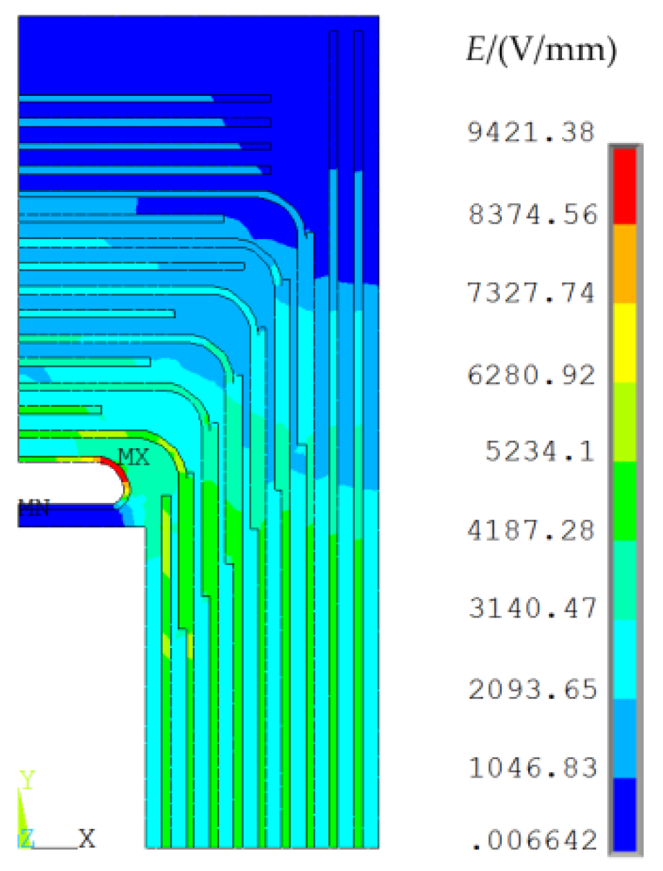
As can be seen in Section 2.1, the maximum electric field intensity emerged at the upper right corner of the electrostatic ring. Therefore, we can select the parameters related to the electrostatic ring as the variables to optimize. The structure and parameters of the electrostatic ring are shown in Figure 4.

Due to the existence of the pressboard, for easy analysis, H is simplified as h, the distance from the top surface of the electrostatic ring (without insulation layer) to the first pressboard above the electrostatic ring. The relationship between the two arcs of the electrostatic ring can be expressed by Equation (6).

$$\{\begin{array}{l}{\theta }_1+{\theta }_2={180}^{°}\\ y_1=T_1-R_1\\ R_2=\frac{(y_1+R_1\ast \cos {\theta }_1-T_2)}{1+\cos {\theta }_1}\\ x_2=x_1+(R_1-R_2)\ast \sin {\theta }_1\\ y_2=y_1+(R_1-R_2)\ast \cos {\theta }_1\end{array}.$$

(6)

Among them, the coordinates of the center of the two arcs are (x₁, y₁) and (x₂, y₂). Values T₁ and T₂ are the ordinate values of the upper and lower surfaces of the electrostatic ring (excluding the insulating layer). As can be seen from the above equation, R₂ and θ₂ can be derived from R₁ and θ₁. Therefore, the four optimization variables R₁, θ₁, R₂, and θ₂ can be simplified into two variables, namely R₁ and θ₁.

The optimization process is demonstrated in Figure 5.

3.1. Taguchi Experiment

Through the above analysis, the Taguchi experiment was carried out with R₁, θ₁, h, s, and w as variables to be optimized. Taking the median values of the variables on both sides and their adjacent values as the impact factors, the impact factors of the optimized parameters are listed in

Table 2. Parameters to be optimized and impact factors.

Parameters	R1/mm	θ1/°	h/mm	s/mm	w/mm
impact factor 1	10	52.5	12.5	2.75	42.5
impact factor 2	14	75	15	3.5	45
impact factor 3	18	97.5	17.5	4.25	47.5

.

The orthogonal table L₉(3⁵) is obtained by the Taguchi method, where L represents an orthogonal matrix; 9 stands for the number of trials; 3 is the number of times each variable is taken, and 5 symbolizes the number of optimization parameters. According to the orthogonal table, the maximum electric field intensity can be achieved by the mutual call between MATLAB and ANSYS, as shown in the

Table 3. Orthogonal matrix and results of L₉(3⁵).

Number of Experiments	R1/mm	θ1/°	h/mm	s/mm	w/mm	Emax/(V/mm)
1	1	1	1	1	2	10385.95
2	1	2	2	2	1	9794.79
3	1	3	3	3	3	9615.61
4	2	1	2	3	1	9170.99
5	2	2	3	1	2	9928.34
6	2	3	1	2	3	9866.17
7	3	1	3	2	3	9681.51
8	3	2	1	3	2	9167.40
9	3	3	2	1	1	9559.65

.

From the results obtained by Table 3, the proportion of each parameter is calculated by Equation (7).

$$EE=3{\displaystyle \sum _{i=1}^3{\left[m_{x_i}(E_i)-m(E)\right]}^2},$$

(7)

where x_i represents R₁, θ₁, h, s, and w; EE is the proportion of each optimization parameter; m_xi(E_i) is the average value of E_max under the ith impact factor of x; and m(E) is the average value of E_max. The proportion of each optimization parameter is listed in

Table 4. Influence proportion of the optimized parameters on E_max.

Parameters	EE	Proportion (%)
R1/mm	325,162.8862	25.0
θ1/mm	20,294.4814	1.6
h/mm	140,533.0000	10.8
s/mm	655,163.7245	50.3
w/mm	160,650.0366	12.3
Total	1,301,804.1290	100

.

It can be seen from

Table 5. Level of test factors by CCD.

Variables	Levels
	−α	−1	0	1	α
R1	5	6	14	22	24
h	5	10	15	20	25
s	0.5	2	3.5	5	6.5
w	35	40	45	50	55

Note: The −α and α levels of R₁ are −1 and 27, respectively, which exceed the range of variation and are appropriately adjusted.

that R₁, h, s, and w have greater influence on the maximum electric field intensity,while θ₁ can be eliminated from the impact variables. The Taguchi method effectively reduced the workload of the numerical analysis of the subsequent response surface. In the following experiment, for the convenience of analysis, the electrostatic ring was divided into two arcs; both of them were 90 degrees. The values R₁, h, s, and w were selected as experimental variables.

3.2. Experimental Data

After determining the experimental variables, the appropriate range of values was selected for the response surface experiment. There are four optimization variables in this experiment, so α=2. The design and combination of the experimental sample points were carried out by the CCD method, as shown in Table 5.

Table 6. Experimental data.

Run	Actual/mm				Coded				Emax	Number of Elements	DOFs
	R1	h	s	w	x1	x2	x3	x4	/(V/mm)
1	6	10	5	40	−1	−1	1	−1	10,909.89	2074	3958
2	24	15	3.5	45	1.571	0	0	0	9154.23	2125	4038
3	13	15	0.5	45	0	0	−2	0	11,831.83	2528	4700
4	20	10	5	40	1	−1	1	−1	8599.39	2081	3967
5	6	20	5	50	−1	1	1	1	11,053.85	2080	3962
6	6	10	2	50	−1	−1	−1	1	12,416.88	2133	4047
7	13	15	3.5	45	0	0	0	0	9664.49	2090	3981
8	13	15	3.5	45	0	0	0	0	9664.49	2090	3981
9	20	20	5	50	1	1	1	1	8870.22	2080	3957
10	13	15	6.5	45	0	0	2	0	9328.45	2087	3983
11	13	5	3.5	45	0	−2	0	0	10,048.23	2131	4060
12	20	20	5	40	1	1	1	−1	8243.91	2082	3963
13	6	20	2	50	−1	1	−1	1	11,789.22	2140	4057
14	6	10	2	40	−1	−1	−1	−1	11,656.15	2128	4044
15	13	15	3.5	45	0	0	0	0	9664.49	2090	3981
16	13	25	3.5	45	0	2	0	0	9151.81	2129	4035
17	17	15	3.5	55	0	0	0	2	10,380.85	2088	3973
18	6	10	5	50	−1	−1	1	1	11,564.39	2076	3959
19	20	20	2	50	1	1	−1	1	10,083.12	2153	4073
20	5	15	3.5	45	−1.413	0	0	0	11,879.20	2102	4004
21	13	15	3.5	45	0	0	0	0	9664.49	2090	3981
22	20	10	2	40	1	−1	−1	−1	9758.90	2137	4053
23	13	15	3.5	45	0	0	0	0	9664.49	2090	3981
24	20	10	2	50	1	−1	−1	1	10,391.28	2147	4006
25	20	10	5	50	1	−1	1	1	9179.16	2079	3961
26	6	20	5	40	−1	1	1	−1	10,354.56	2082	3970
27	13	15	3.5	45	0	0	0	0	9664.49	2090	3981
28	20	20	2	40	1	1	−1	−1	9314.94	2145	4064
29	13	15	3.5	35	0	0	0	−2	9077.65	2086	3977
30	6	20	2	40	−1	1	−1	−1	11,046.17	2131	4047

is the experimental data results of the sample points which were obtained by calling each other between ANSYS and MATLAB.

The last two columns of Table 6 are the number of elements and nodes (degrees of freedom) of the local finite element model in Figure 1b. According to statistics, it took only 61.8 seconds to complete the above 30 CCD experiments. Without the CCD method, 625 RSM experiments would be required. Thus, by using CCD method, the optimization efficiency was greatly improved.

Referring to the above data, the coefficients of the response surface model were obtained by Equation (5). We can get the initial response surface model from

Table 7. Coefficients of RSM model.

Factor	df	Standard Error	95% CI Low	95% CI High	Coefficient Estimate
Intercept	1	54.99	9583.37	9817.79	12419.312
R1	1	31.52	−1120.49	−986.12	−371.458
h	1	28.29	−290.01	−169.40	−55.687
s	1	28.29	−588.97	−468.36	−783.092
w	1	28.29	275.97	396.58	84.888
R1h	1	34.65	−18.43	129.30	1.584
R1s	1	34.65	−175.73	−28.00	−9.701
R1w	1	34.65	−89.55	58.18	−0.448
hs	1	34.65	−57.65	90.08	2.162
hw	1	34.65	−60.77	86.95	0.524
sw	1	34.65	−95.39	52.33	−2.870
R12	1	42.70	382.68	564.71	9.667
h2	1	26.20	−90.83	20.87	−1.399
s2	1	26.20	154.20	265.90	93.357
w2	1	26.20	−58.52	53.18	−0.107

.

3.3. Analysis of Variance

The ANOVA table summarizes the results of the variance analysis, as shown in

Table 8. Analysis of variance.

Source of Variation	Sum of Squares	Degrees of Freedom	Mean Square	F0	p-Value	Significance
Regression	3.468 × 107	14	2.477 × 106	128.92	<0.0001	***
R1	2.146 × 107	1	2.146 × 107	1116.64	<0.0001	***
h	1.266 × 106	1	1.266 × 106	65.91	<0.0001	***
s	6.708 × 106	1	6.708 × 106	349.10	<0.0001	***
w	2.714 × 106	1	2.714 × 106	141.25	<0.0001	***
R1h	4.917 × 104	1	4.917 × 104	2.56	0.1305
R1s	1.660 × 105	1	1.660 × 105	8.64	0.0101	*
R1w	3.936 × 103	1	3.936 × 103	0.20	0.6573
hs	4.207 × 103	1	4.207 × 103	0.22	0.6466
hw	2.741 × 103	1	2.741 × 103	0.14	0.7109
sw	7.415 × 103	1	7.415 × 103	0.39	0.5438
R12	2.365 × 106	1	2.365 × 106	123.06	<0.0001	***
h2	3.424 × 104	1	3.424 × 104	1.78	0.2018
s2	1.235 × 106	1	1.235 × 106	64.26	<0.0001	***
w2	199.590	1	199.590	0.01	0.9202
Lack of Fit	2.882 × 105	15	2.882 × 105
Pure Error	0.000	5	0.000
Total	3.497 × 107	29

Note: *** Extremely significant; ** Very significant; * Significant

.

As shown in Table 8, the p-value of the regression model was less than 0.0001, which means that the choice of the quadratic polynomial model is reasonable, and the relationship between the maximum electric field intensity value, y, and the regression equation is extremely significant. Thus, the null hypothesis, H₀, is not valid and can be rejected. The p-value of all linear terms were less than 0.0001, indicating that each variable in R₁, h, s, and w is an extremely significant factor affecting the optimization objective. Except that the interaction between R₁ and s was significant, the p-value of each of the other two was greater than 0.05, demonstrating the interaction between the two has little effect on the response. The p-values of the quadratic terms R₁² and s²were less than 0.0001, and the significance was higher than the other two, which is an extremely significant factor. In addition, $R_{adj}^2$ is 0.9841, which is very close to 1. The model can explain 98.41% of the test changes and better reflect the law of data changes with less experimental error and better fitting. Furthermore, from the confidence interval listed in Table 8, the significant items are also R₁, h, s, w, R₁s, R₁², and s², for the upper and lower bounds of their confidence intervals do not contain zero.

3.4. Diagnostic Analysis

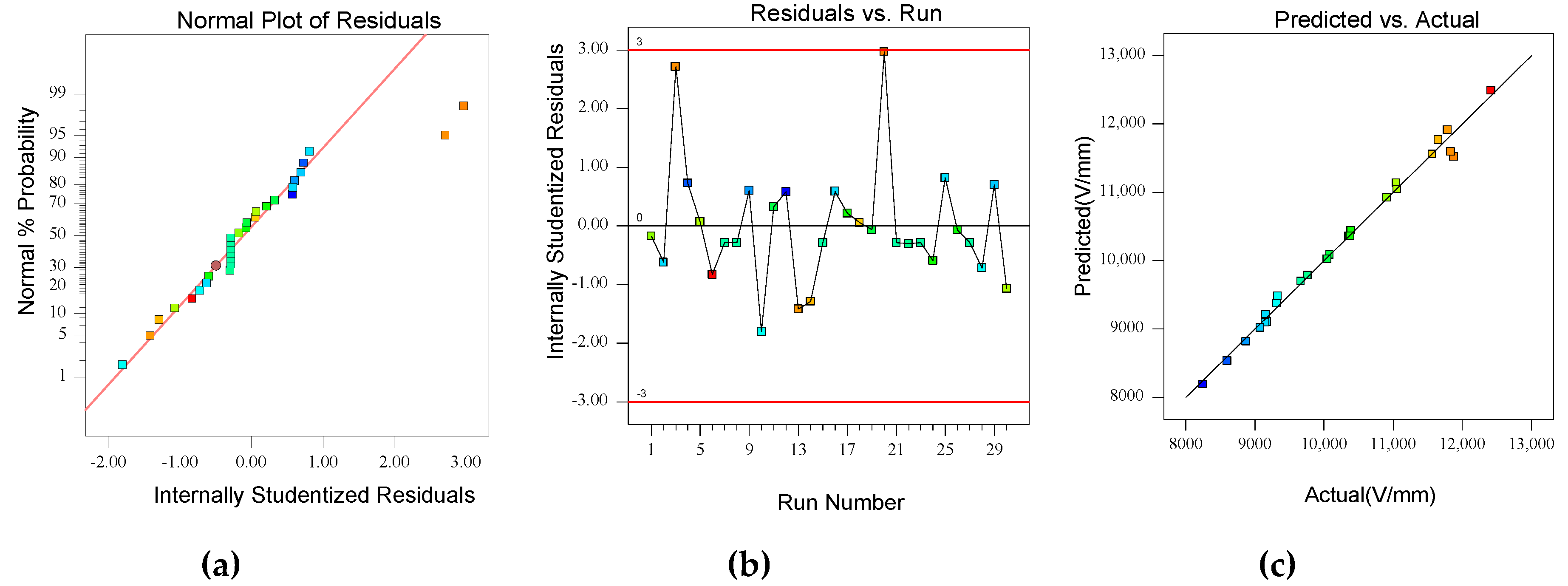
To verify the applicability of the model, the diagnostic analysis was generally made by making the regression analysis and giving some diagnostic plots.

The design of the normal probability plot made the cumulative normal distribution a straight line. In Figure 6a, the points on the normal probability plot were approximately distributed in a straight line, which indicates the accuracy of the data for calculating the electric field intensity.

As can be seen from the residuals versus run plot in Figure 6b, the residuals of runs were distributed within the prescribed appropriate range, which implies that choosing the quadratic polynomial as the response surface function is particularly suitable. In Figure 6c and

Table 9. Comparisons between predicted and actual values.

Run	Actual Values/(V/mm)	Predicted Values/(V/mm)
1	10,909.89	10,924.76
2	9154.23	9215.12
3	11,831.83	11,598.13
4	8599.39	8534.92
5	11,053.85	11,047.78
6	12,416.88	12,488.54
7	9664.49	9700.58
8	9664.49	9700.58
9	8870.22	8816.94
10	9328.45	9483.46
11	10,048.23	10,020.08
12	8243.91	8192.64
13	11,789.22	11,912.01
14	11,656.15	11,767.75
15	9664.49	9700.58
16	9151.81	9101.26
17	10,380.85	10,362.45
18	11,564.39	11,559.45
19	10,083.12	10,088.63
20	11,879.20	11,523.06
21	9664.49	9700.58
22	9758.90	9785.36
23	9664.49	9700.58
24	10,391.28	10,443.42
25	9179.16	9106.87
26	10,354.56	10,360.74
27	9664.49	9700.58
28	9314.94	9378.21
29	9077.65	9017.35
30	11,046.17	11,138.85

, there was a good correlation between the predicted value and the actual value, which indicates that the polynomial model has a good predictive ability. In a word, the response surface model adopted in this study is acceptable.

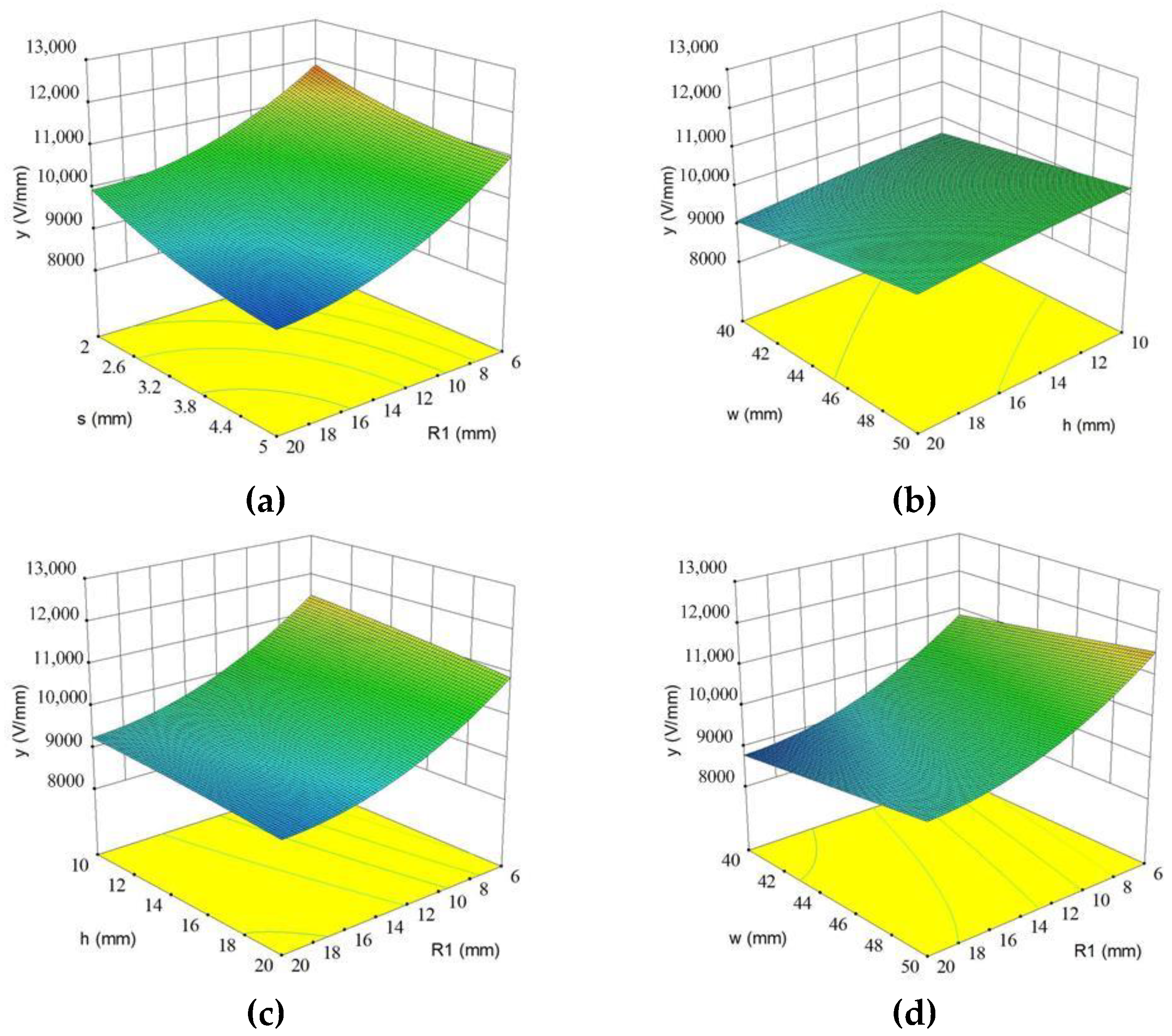
3.5. 3-D Response Surface Analysis

For a better demonstration of the influence of the interaction between two variables, the 3-D plots were adopted. If the interaction has a significant impact on the response surface, the variation of 3-D plot will be accordingly large.

Figure 7a shows that when R₁ and s interact, if we fix one of the variables and increase the other variable, the maximum electric field intensity will decrease. As can be seen from the trend of the surface graph, the maximum electric field intensity decreased faster with R₁ than with s, indicating that R₁ has a greater influence on the response value. Comparing Figure 7a with Figure 7b, the response surface of Figure 7b fluctuated slightly, which means that the change of the interaction term hw has no significant effect on the maximum electric field intensity. Similarly, hs and sw are not significant factors either.

As can be seen from Figure 7c,d, compared with s and w, the change of the maximum electric field intensity was larger with the change of R₁. The maximum electric field intensity increases with the increase of w, which has negative effects on the model. Therefore, in the structural design process, a smaller starting position w should be selected as far as possible within a reasonable range. From the variation range of the two figures, the interactions between R₁ and h, R₁, and w may be a significant factor affecting the maximum electric field intensity. However, since their p-values in Table 8 are little larger than 0.05, R₁h and R₁w can be considered insignificant factors.

Through the above analysis, the insignificant factors, such as R₁h, R₁w, hs, hw, sw, h², and w², are removed, and the final response surface equation with a higher prediction ability is shown in Equation (8).

$$\begin{array}{l}y=12419.312-371.458\ast R_1-55.687\ast h-783.092\ast s+84.888\ast w\\ -9.701\ast R_1\ast s+9.667\ast R_1{}^2+93.357\ast s^2\end{array}$$

(8)

4. Results and Discussion

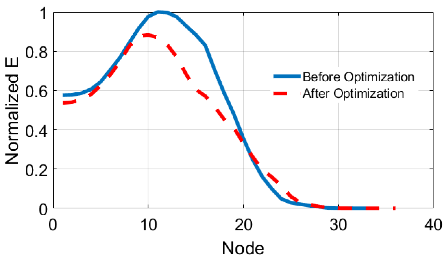
It is an important goal of the response surface optimization to get the optimal results with the appropriate values assigned to each variable. Equation (8) is the quadratic response surface model with single objective optimization, which can be solved quickly by quadratic programming. By comparing the maximum electric field intensities on the electrostatic ring before and after optimization in Figure 8, the decrease of the maximum electric field intensity can be observed more intuitively. The result shows that the maximum electric field intensity has been significantly reduced.

In order to verify the validity of the RSM, we compared the result of RSM with that of traditional FEM. The FEM taking much time and requiring many experiments, to ensure the fairness of the experiment and save the calculation time, thirty experiments were carried out by using the FEM. As can be seen from

Table 10. Optimization results.

Before and After Optimization	Variables				Emax (V/mm)	Decline Rate (%)	Experimental Time(s)
	R1(mm)	h(mm)	s(mm)	w(mm)
Before Optimization	18	15	4	48	9303.30	-
FEM	22	20	5	40	8219.83	11.6	2400
RSM	22	20	5	40	8192.64	12.1	61.8

, the results obtained by RSM and FEM were consistent, while the time the of RSM experiments was much less, which demonstrates the effectiveness of RSM and also shows the high optimization efficiency and good prediction ability of this method.

In Figure 9, a comparison of the variations of variables predicted by the FEM and those actually obtained by the RSM was made. It can be observed that the variations of variables in this paper are monotonic, so FEM can obtain the optimal results by inference in this special case. However, this method is no longer applicable when the variables are not monotonic. The RSM has a wider range for applications and the result obtained by it is more rigorous and convincing.

5. Conclusions

In this paper, the response surface methodology, Taguchi method, and ANSYS parametric modeling language were combined to optimize the electrostatic ring of a 500 kV power transformer. The APDL extracted the maximum electric field intensity automatically and the mutual calls between MATLAB and ANSYS solved the problem of repeated manual modeling and meshing in traditional methods. To avoid the increased calculating workload of developing experiments aroused by irrelevant variables, the Taguchi method was utilized to filter the variables before making response surface experiments, by which the optimization process was effectively simplified. The experimental points were constructed by the experimental design method of CCD, and the response surface model was then obtained. In order to ensure the accuracy and predictability of the model, the response surface model was analyzed by ANOVA, diagnostic analysis, and the significance test of regression, and the final response surface equation was determined. Comparing the optimization results with the traditional finite element method, on the premise of ensuring accuracy, the proposed method in this paper has a higher optimization efficiency.

In general, the structure of the electrostatic ring is optimized more systematically and completely through the Taguchi method and response surface experiments. The feasibility and efficiency of this method were verified, which provides a new and more systematic, fast, and efficient way for the optimization of the transformer insulation structure.