Research of Adaptive Extended Kalman Filter-Based SOC Estimator for Frequency Regulation ESS

 , , , , and
Abstract
1. Introduction
2. Design of Operation Algorithm for FR ESS and Power Characteristics Analysis
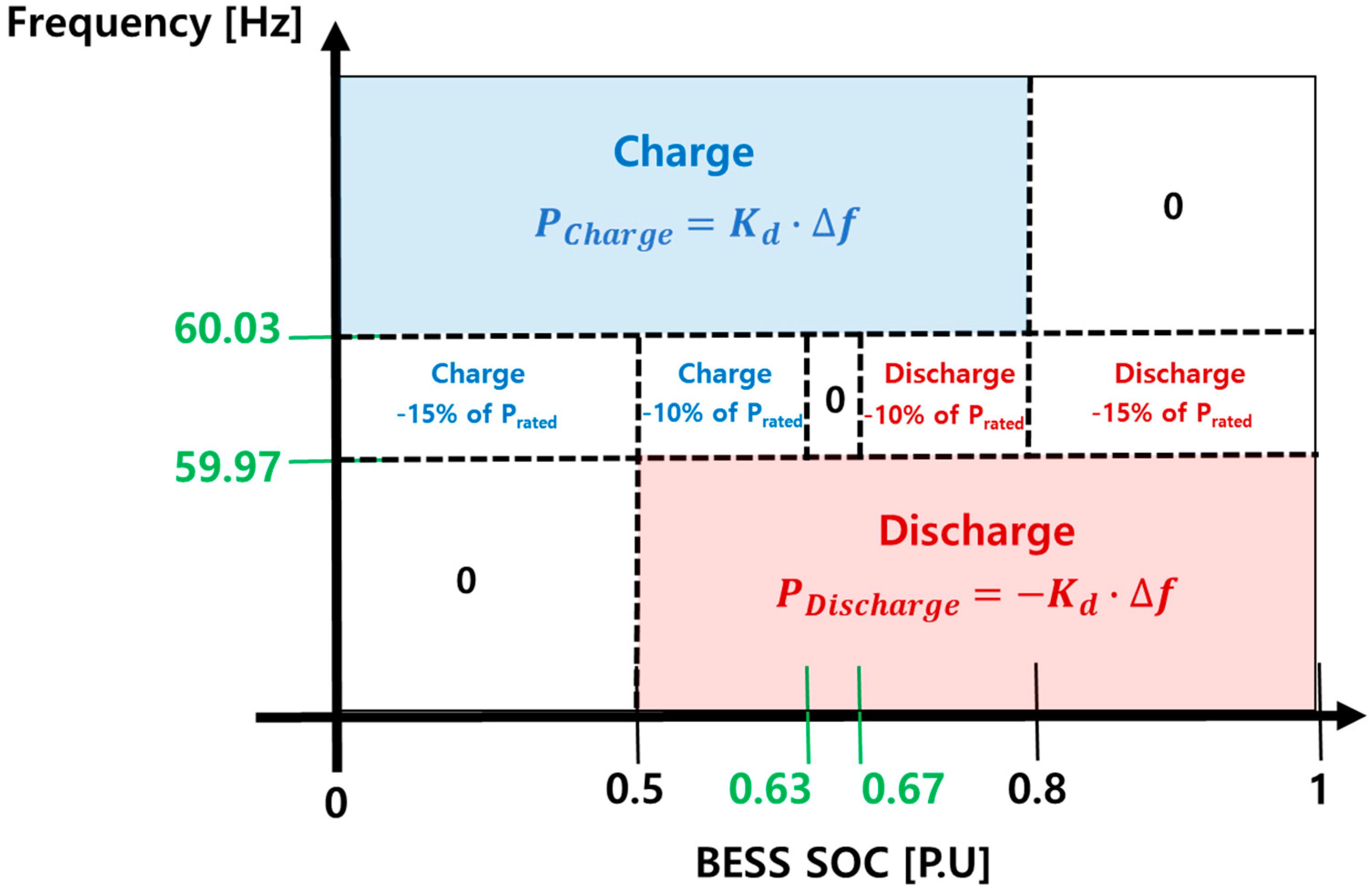
2.1. Operation Algorithm Design of Frequency Regulation ESS
3. Performance Verification of SOC Estimation Using Adaptive Extended Kalman Filter
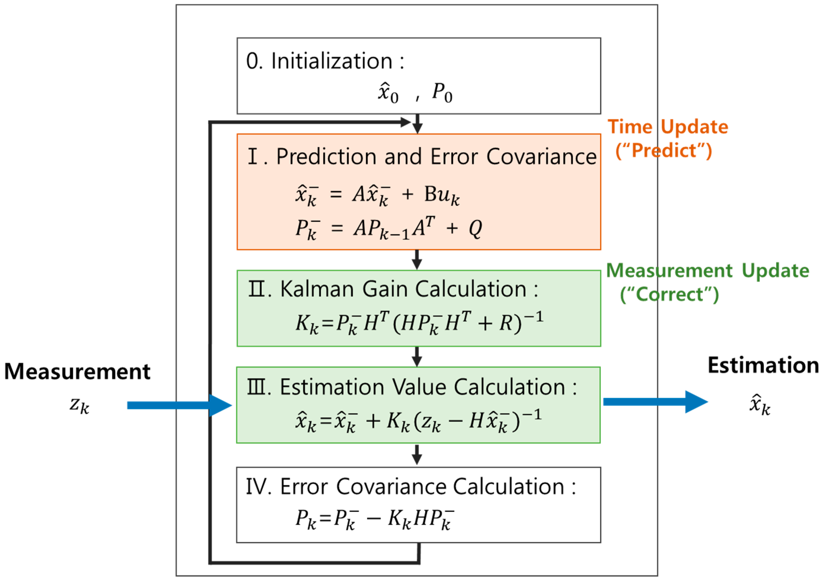
3.1. Extended Kalman Filter Algorithm Design
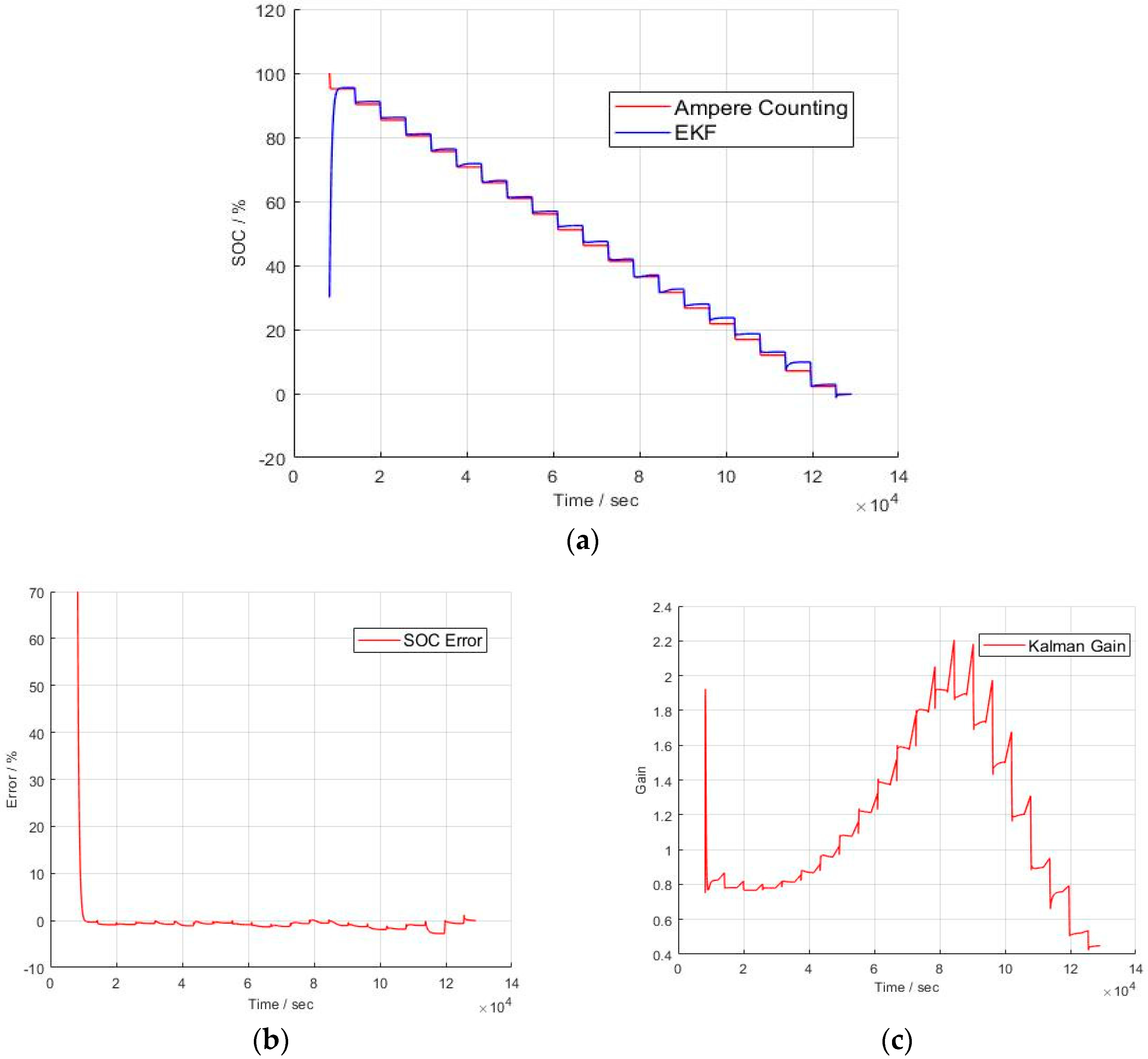
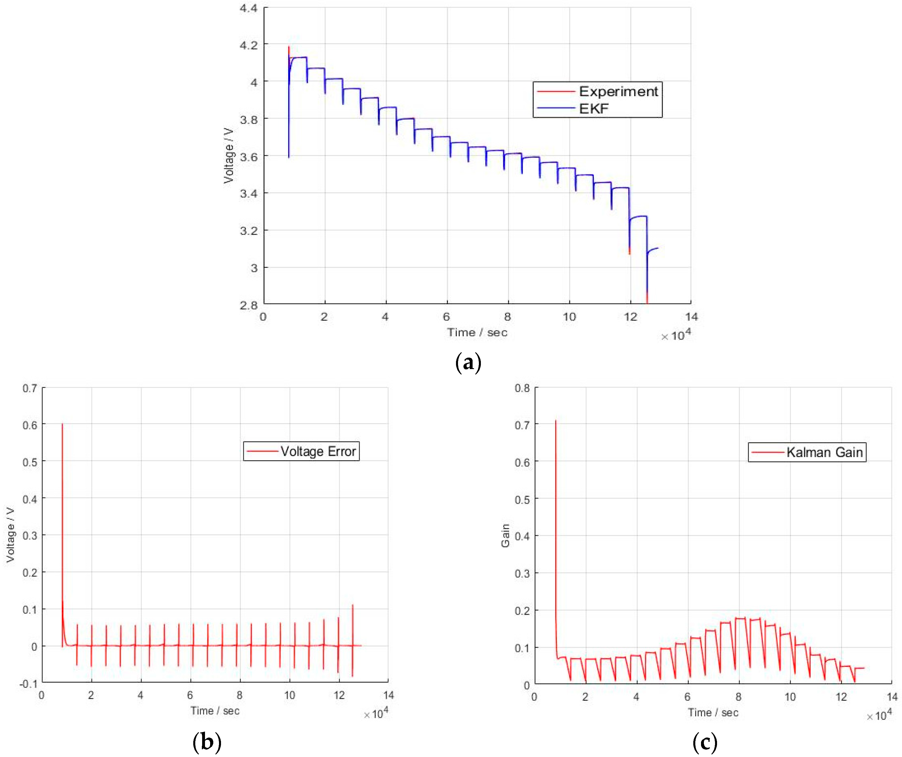
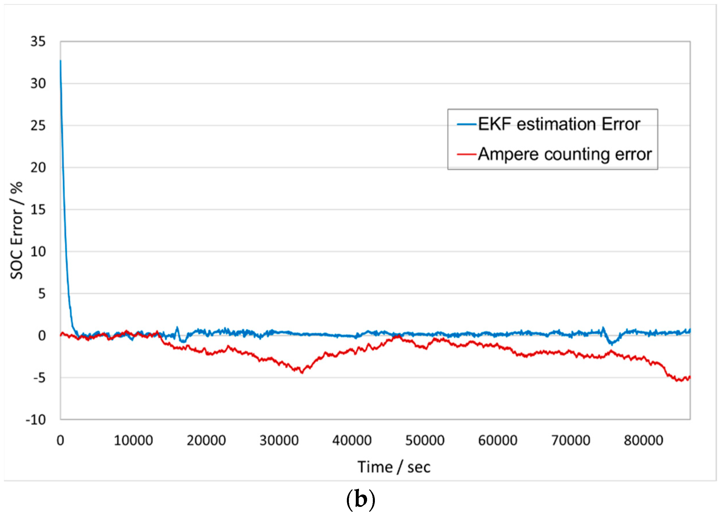
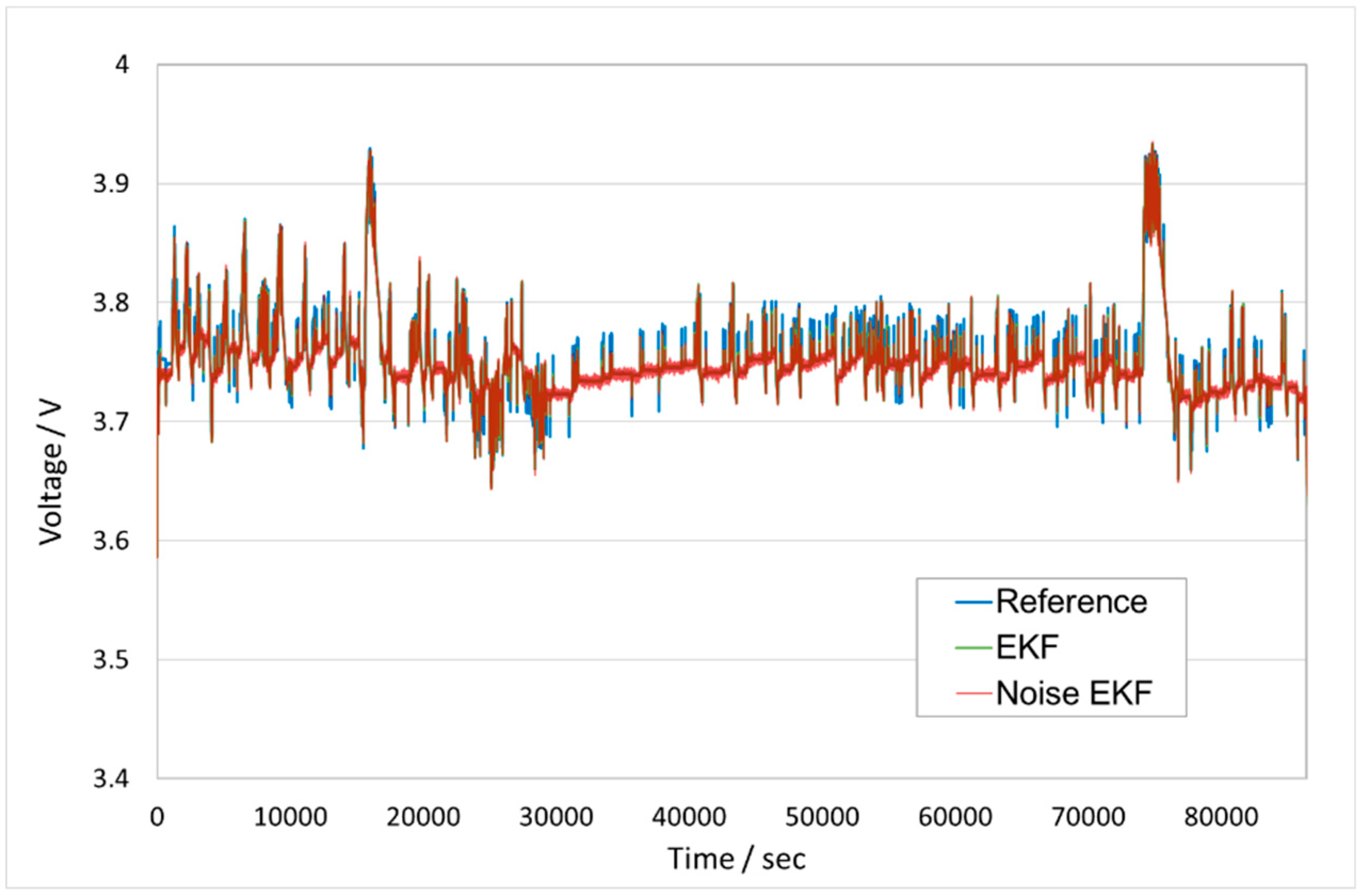
3.2. SOC Estimation of Frequency Regulation ESS Using Extended Kalman Filter
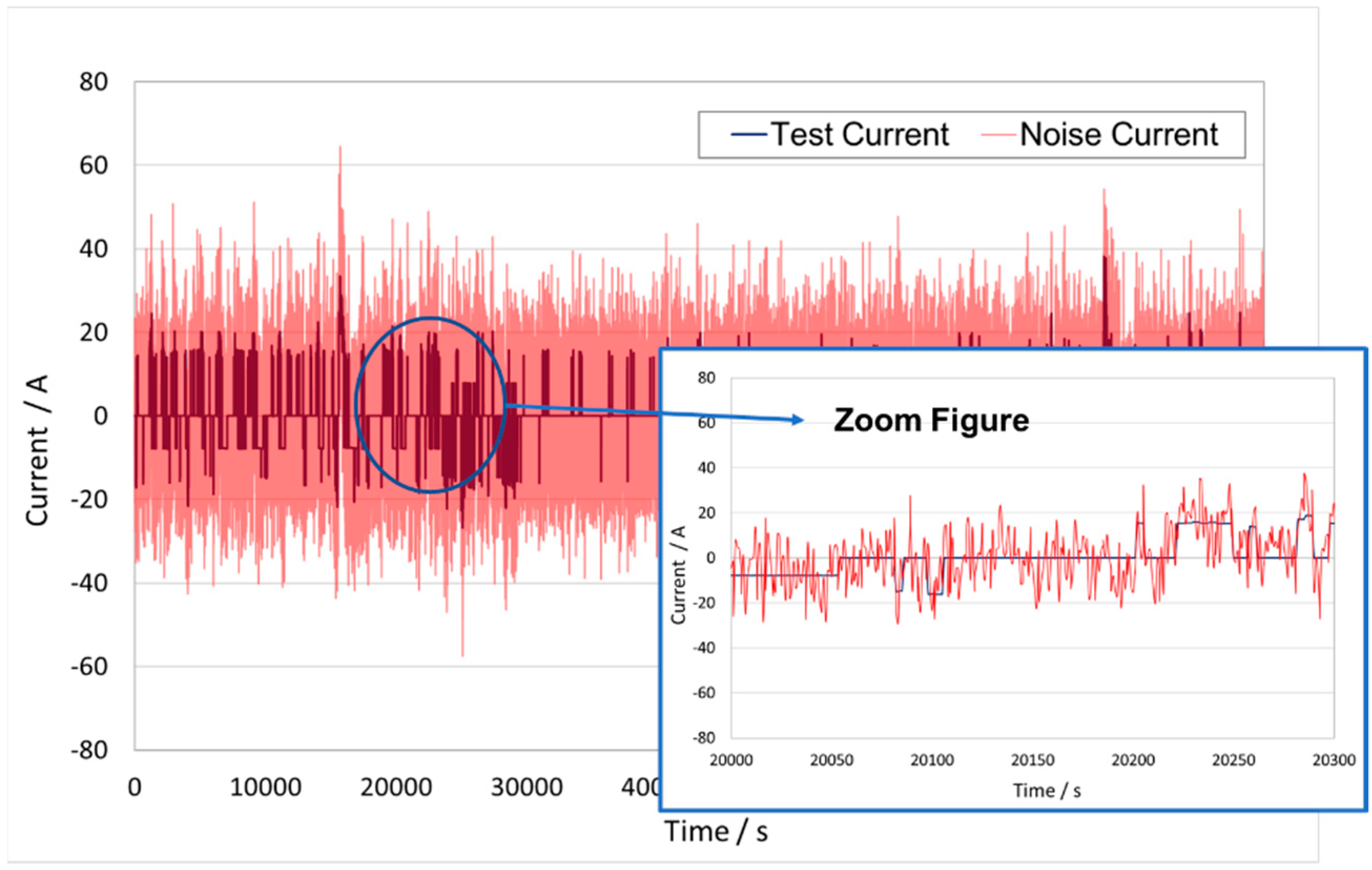
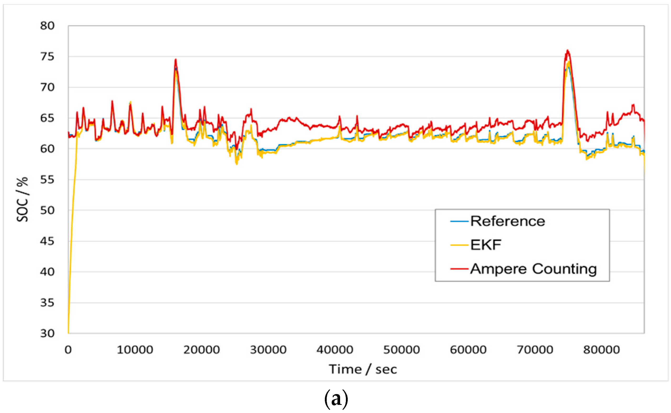
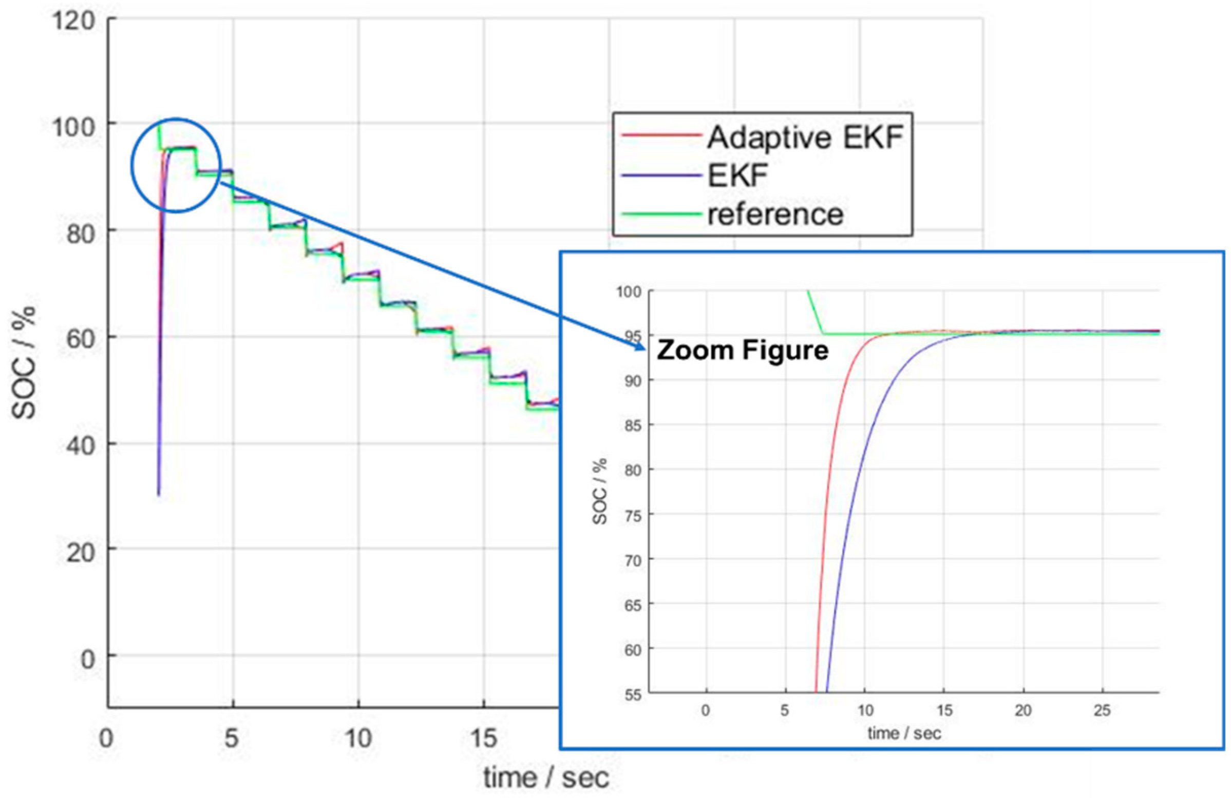
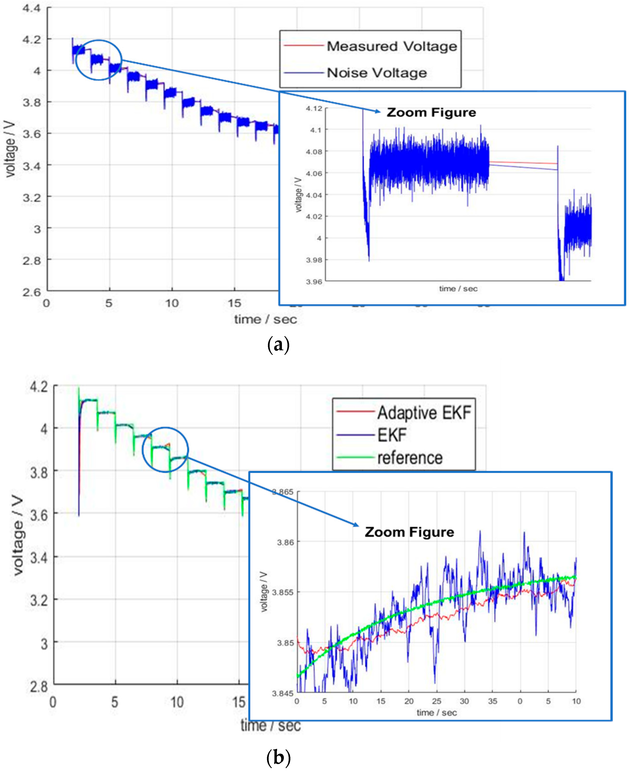
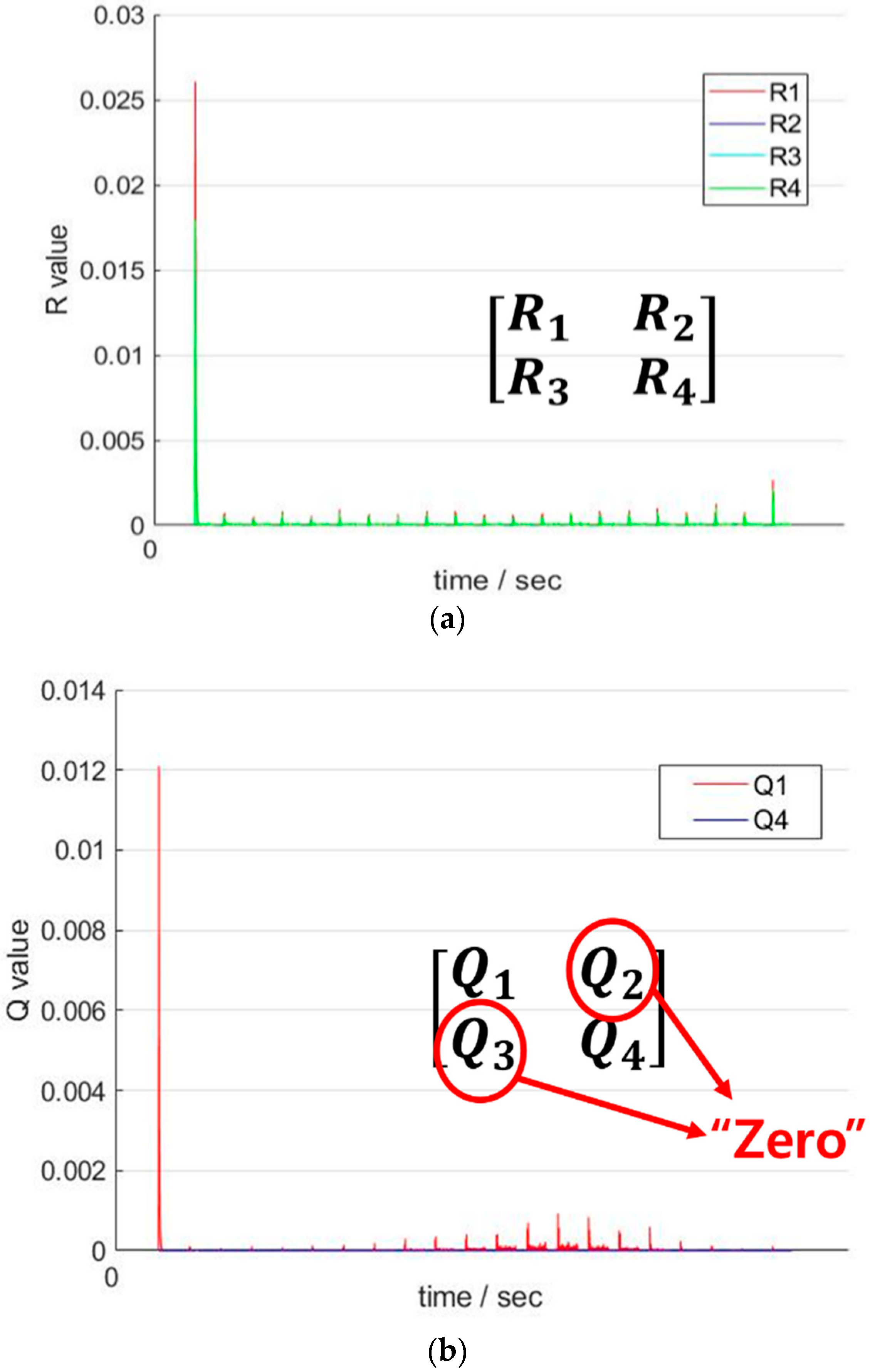
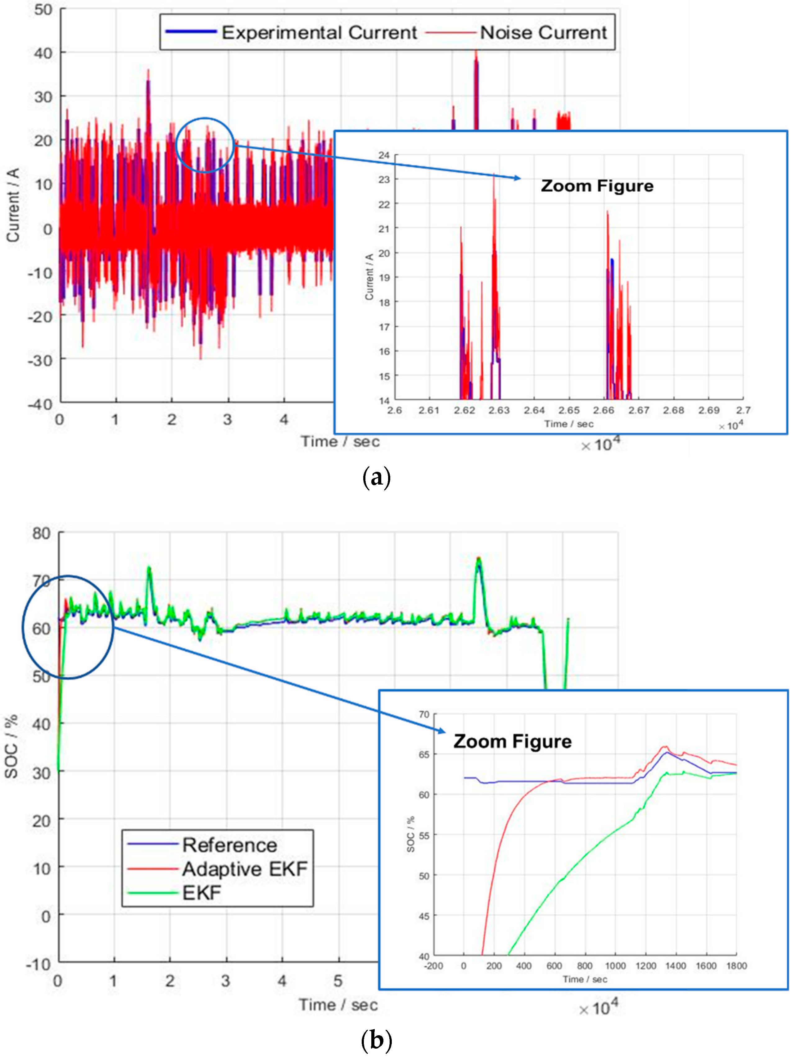
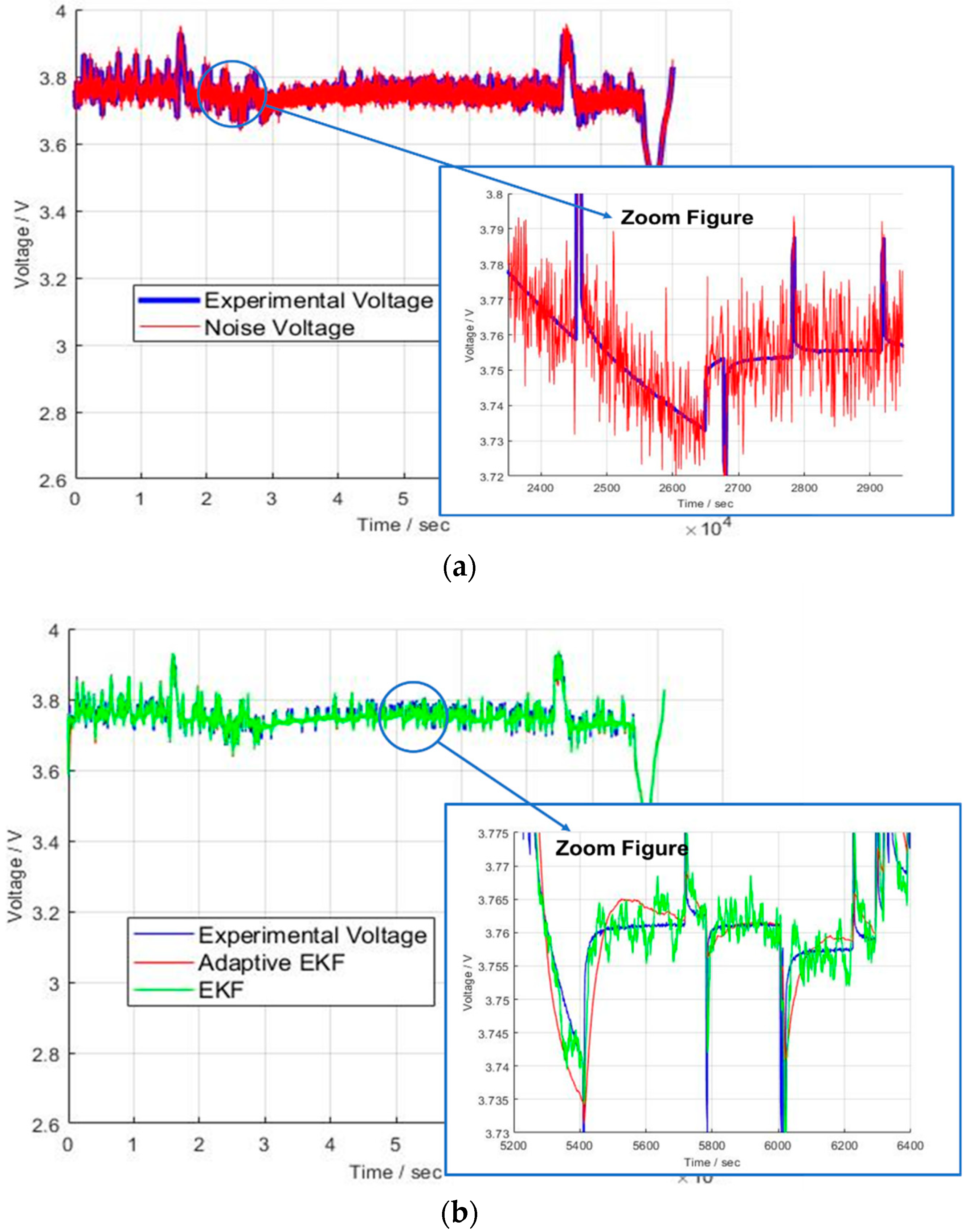
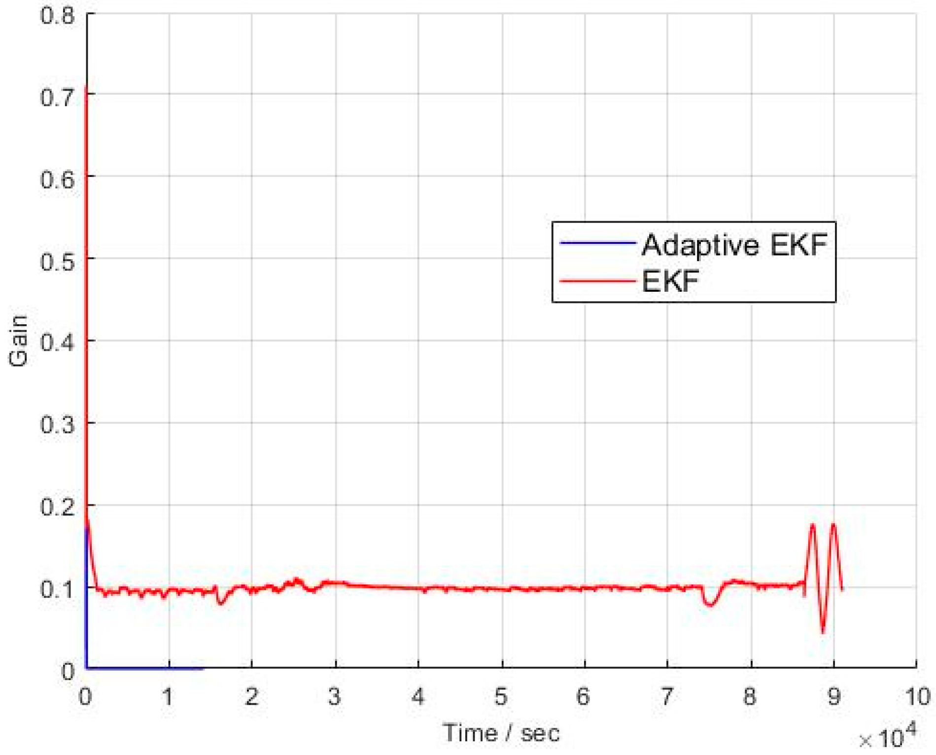
3.3. SOC Estimation Using Adaptive Extended Kalman Filter
4. Conclusions
Author Contributions
Funding
Conflicts of Interest
Abbreviations
| ESS | Energy Storage System |
| BESS | Battery Energy Storage System |
| OCV | Open Circuit Voltage |
| SOC | State Of Charge |
| FR | Frequency Regulation |
| ECM | Equivalent Circuit Model |
| KF | Kalman Filter |
| EKF | Extended Kalman Filter |
| AEKF | Adaptive Extended Kalman Filter |
| UKF | Unscented Kalman Filter |
| PF | Particle Filter |
| SMO | Sliding mode observer |
| UDDS | Urban Dynamometer Driving Schedule |
| NN | Neural Network |
| DNN | Deep Neural Network |
| SVM | Support Vector Machine |
References
- International Electrotechnical Commission. Electric Energy Storage Device; International Electrotechnical Commission: Geneva, Switzerland, 2016. [Google Scholar]
- Korea Power Exchange. Procurement of Operating Reserve Considering Characteristics of ESS for Frequency Regulation; Korea Power Exchange: NaJu, Korea, 2017. [Google Scholar]
- Yun, J.Y.; Yu, G.R.; Kook, K.S.; Rho, D.H.; Chang, B.H. SOC-based control strategy of battery energy storage system for power system frequency regulation. Korean Inst. Electr. Eng. 2014, 63, 622–628. [Google Scholar]
- Greenwood, D.; Lim, K.; Patsios, C.; Lyons, P.; Lim, Y.; Taylor, P. Frequency response service designed for energy storage. Appl. Energy 2017, 203, 115–127. [Google Scholar] [CrossRef]
- Brivio, C.; Mandelli, S.; Merlo, M. Battery energy storage system for primary control reserve and energy arbitrage. Sustain. Energy Grids Netw. 2016, 6, 152–165. [Google Scholar] [CrossRef]
- Cheng, M.; Sami, S.S.; Wu, J. Benefits of using virtual energy storage system for power system frequency response. Appl. Energy 2017, 194, 376–385. [Google Scholar] [CrossRef]
- Cho, S.M.; Jang, B.H.; Yoon, Y.B.; Jeon, W.J.; Kim, C.W. Operation of battery energy storage system for governor free and its effect. Trans. Korean Inst. Electr. Eng. 2015, 64, 16–22. [Google Scholar] [CrossRef]
- Swierczynski, M.; Stroe, D.I.; Stan, A.I.; Teodorescu, R. Field tests experience from 1.6 MW/400 kWh Li-ion battery energy storage system providing primary frequency regulation service. In Proceedings of the IEEE PES Innovative Smart Grid Technologies Europe (ISGT Europe), Lyngby, Denmark, 6–9 October 2013. [Google Scholar]
- Moon, H.J.; Yun, A.Y.; Kim, E.S.; Moon, S.I. An analysis of energy storage systems for primary frequency control of power systems in South Korea. In Proceedings of the 3rd International Conference on Energy and Environment Research, Barcelona, Spain, 7–11 September 2016. [Google Scholar]
- Patsios, C.; Wub, B.; Chatzinikolaoud, E.; Rogersd, D.J.; Wade, N.; Brandon, N.P.; Taylor, P. An integrated approach for the analysis and control of grid connected energy storage systems. J. Energy Storage 2016, 5, 48–61. [Google Scholar] [CrossRef]
- Delfanti, M.; Falabretti, D.; Merlo, M.; Monfredini, G. Distributed generation integration in the electric grid: Energy storage system for frequency control. J. Appl. Math. 2014, 2014, 198427. [Google Scholar] [CrossRef]
- Izadkhast, S.; Garcia-Gonzalez, P.; Frias, P. An aggregate model of plug-in electric vehicles for primary frequency control. IEEE Trans. Power Syst. 2015, 30, 1475–1482. [Google Scholar] [CrossRef]
- Koller, M.; Borsche, T.; Ulbig, A.; Andersson, G. Review of grid applications with the Zurich 1MW battery energy storage system. Electr. Power Syst. Res. 2015, 120, 128–135. [Google Scholar] [CrossRef]
- Zhao, H.; Wu, Q.; Hu, S.; Xu, H.; Rasmussen, C.N. Review of energy storage system for wind power integration support. Appl. Energy 2015, 137, 545–553. [Google Scholar] [CrossRef]
- Cheng, M.; Wu, J.; Galsworthy, S.; Jenkins, N.; Hung, W. Availability of load to provide frequency response in the great Britain power system. In Proceedings of the 2014 Power Systems Computation Conference, Wroclaw, Poland, 18–22 August 2014. [Google Scholar]
- Behrangrad, M. A review of demand side management business models in the electricity market. Renew. Sustain. Energy Rev. 2015, 47, 270–283. [Google Scholar] [CrossRef]
- Julien, C.M.; Mauger, A.; Zaghib, K.; Groult, H. Comparative issues of cathode materials for Li-ion batteries. Inorganics 2014, 2, 132–154. [Google Scholar] [CrossRef]
- Nitta, N.; Wu, F.; Lee, J.T.; Yushin, G. Li-ion battery materials: Present and future. Mater. Today 2015, 18, 252–264. [Google Scholar] [CrossRef]
- Noh, H.J. Comparison of the structural and electrochemical properties of layered Li[NixCoyMnz]O2 (x = 1/3, 0.5, 0.6, 0.7, 0.8 and 0.85) cathode material for lithium-ion batteries. J. Power Sources 2013, 233, 121–130. [Google Scholar] [CrossRef]
- Jiang, L.; Wang, Q.; Suna, J. Electrochemical performance and thermal stability analysis of LiNixCoyMnzO2 cathode based on a composite safety electrolyte. J. Hazard. Mater. 2018, 351, 260–269. [Google Scholar] [CrossRef] [PubMed]
- Wei, Z.; Zhao, J.; Ji, D.; Tseng, K. A multi-timescale estimator for battery state of charge and capacity dual estimation based on an online identified model. Appl. Energy 2017, 204, 1264–1274. [Google Scholar] [CrossRef]
- Wei, Z.; Meng, S.; Xiong, B.; Ji, D.; Tseng, K. Enhanced online model identification and state of charge estimation for lithium-ion battery with a FBCRLS based observer. Appl. Energy 2016, 181, 332–341. [Google Scholar] [CrossRef]
- Alexandros, N.; Joris, J.; Joris, H.; Shovon, G.; Noshin, O.; Peter, V.; Joeri, V. Complete cell-level lithium-ion electrical ECM model for different chemistries (NMC, LFP, LTO) and temperatures (−5 °C to 45 °C)—Optimized modelling techniques. Electr. Power Energy Syst. 2018, 98, 133–146. [Google Scholar]
- Kang, L.; Zhao, X.; Ma, J. A new neural network model for the state-of-charge estimation in the battery degradation process. Appl. Energy 2014, 121, 20–27. [Google Scholar] [CrossRef]
- Ephrem, C.; Phillip, K.; Matthias, P.; Ali, E. State-of-charge estimation of Li-ion batteries using deep neural networks: A machine learning approach. J. Power Sources 2018, 400, 242–255. [Google Scholar]
- Alvarez, J.C.; Garcia, P.J.; Juez, F.J.; Sanchez, F.; Gonzalez, M.; Roqueni, M.N. Battery state-of-charge estimator using the SVM technique. Appl. Math. Model. 2013, 37, 6244–6253. [Google Scholar] [CrossRef]
- Chaturvedi, N.; Klein, R. Algorithms for advanced battery-management systems. Control Syst. 2010, 30, 49–68. [Google Scholar]
- Hairong, W.; Zhihong, D.; Bo, F.; Hongbin, M.; Yuanqing, X. An adaptive Kalman filter estimating process noise covariance. Neurocomputing 2017, 223, 12–17. [Google Scholar]
- Pan, H.; Lü, Z.; Lin, W.; Li, J.; Chen, L. State of charge estimation of lithium-ion batteries using a grey extended Kalman filter and a novel open-circuit voltage model. Energy 2017, 138, 764–775. [Google Scholar] [CrossRef]
- Hannan, M.A.; Lipu, M.S.H.; Hussain, A.; Mohamed, A. A review of lithium-ion battery state of charge estimation and management system in electric vehicle applications: Challenges and recommendations. Renew. Sustain. Energy Rev. 2017, 78, 834–854. [Google Scholar] [CrossRef]
- Hou, J.; Yang, Y.; He, H.; Gao, T. Adaptive dual extended Kalman filter based on variational bayesian approximation for joint estimation of lithium-ion battery state of charge and model parameters. Appl. Sci. 2019, 9, 1726. [Google Scholar] [CrossRef]
- Partovibakhsh, M.; Guangjun, L. An adaptive unscented Kalman filtering approach for online estimation of model parameters and state-of-charge of lithium-ion batteries for autonomous mobile robots. IEEE Trans. Control Syst. Technol. 2015, 23, 357–363. [Google Scholar] [CrossRef]
- Nejad, S.; Gladwin, D.T.; Stone, D.A. On-chip implementation of extended Kalman filter for adaptive battery states monitoring. In Proceedings of the 42nd Annual Conference of the IEEE Industrial Electronics Society, Florence, Italy, 23–26 October 2016; pp. 5513–5518. [Google Scholar]
- Zeng, Z.; Tian, J.; Li, D.; Tian, Y. An online state of charge estimation algorithm for lithium-ion batteries using an improved adaptive cubature Kalman filter. Energies 2018, 11, 59. [Google Scholar] [CrossRef]
- He, H.; Xiong, R.; Zhang, X.; Sun, F.; Fan, J. State-of-charge estimation of the Lithium-ion battery using an adaptive extended Kalman filter based on an improved Thevenin model. IEEE Trans. Veh. Technol. 2011, 60, 1461–1469. [Google Scholar]
- Plett, G.L. Extended Kalman filtering for battery management systems of LiPB-based HEV battery packs—Part 1. Background. J. Power Sources 2004, 134, 252–261. [Google Scholar] [CrossRef]
- Yang, D.; Lu, C.; Qi, G. An improved electric model with online parameters correction for large Li-ion battery packs. Int. J. Comput. Electr. Eng. 2013, 5, 330. [Google Scholar] [CrossRef]
- Yu, D.X.; Gao, Y.X. SOC estimation of Lithium-ion battery based on Kalman filter algorithm. In Proceedings of the 2nd International Conference on Computer Science and Electronics Engineering (ICCSEE 2013), Hangzhou, China, 22–23 March 2013. [Google Scholar]
- Lee, J.; Nam, O.; Cho, B. Li-ion battery soc estimation method based on the reduced order extended Kalman filtering. J. Power Sources 2007, 174, 9–15. [Google Scholar] [CrossRef]
- Li, Y.; Wang, C.; Gong, J. A multi-model probability SOC fusion estimation approach using an improved adaptive unscented Kalman filter technique. Energy 2017, 141, 1402–1415. [Google Scholar] [CrossRef]
- Peng, S.; Chen, C.; Shi, H.; Yao, Z. State of charge estimation of battery energy storage systems based on adaptive unscented Kalman filter with a noise statistics estimator. IEEE Access 2017, 5, 13202–13212. [Google Scholar] [CrossRef]


| Parameter | Value |
|---|---|
| Reference Frequency (Hz) | 60 |
| Dead Band (Hz) | ±0.03 |
| Center SOC (%) | 65 |
| SOC Operation Range (%) | ±2 |
| Rated Power (W) | 292 |
| Nominal Energy (Wh) | 73 |
| SOC Recovery Power “50 < SOC < 80” (%) | 10% (of rated power) |
| SOC Recovery Power “SOC < 50, 80 < SOC” (%) | 15% (of rated power) |
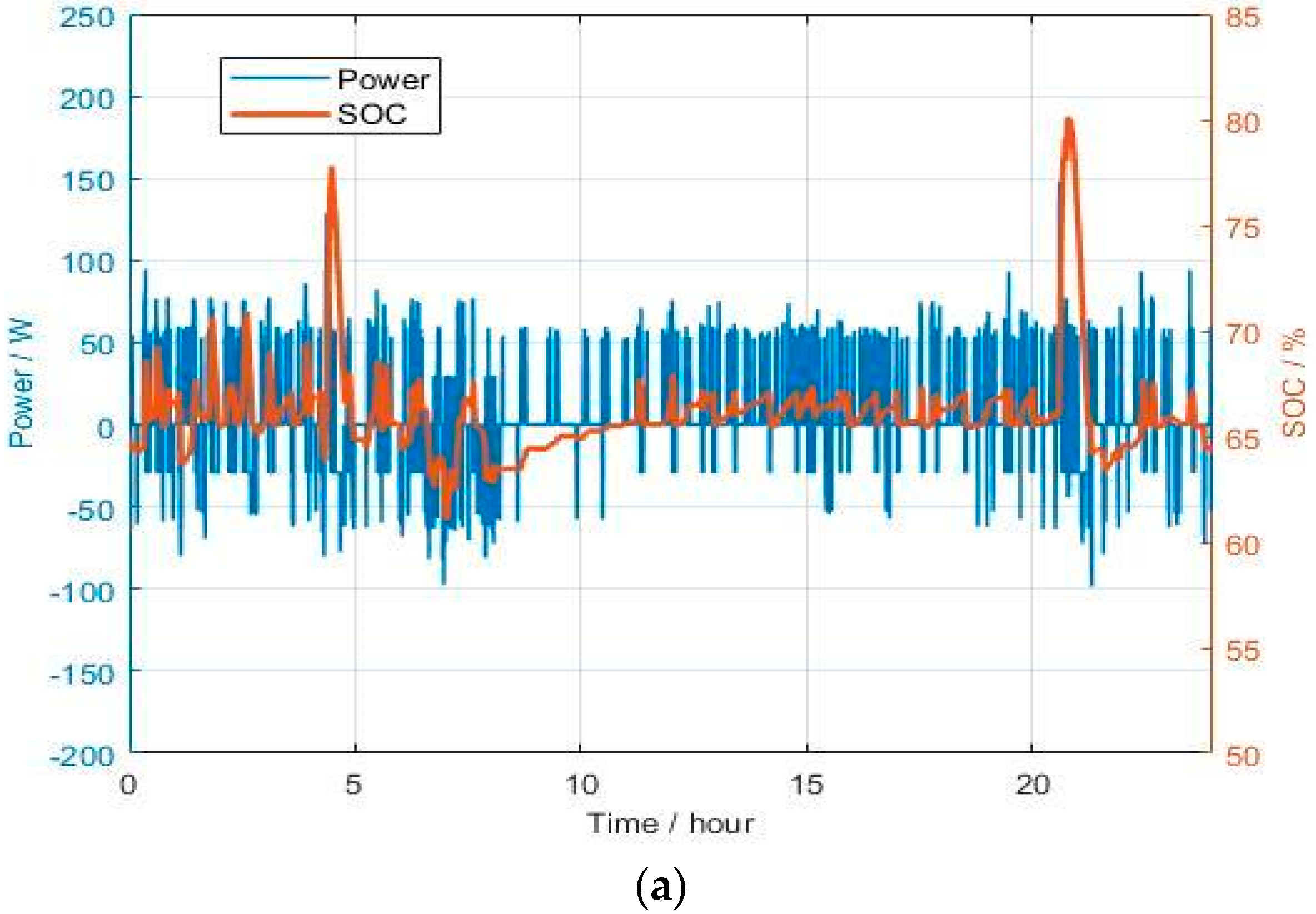
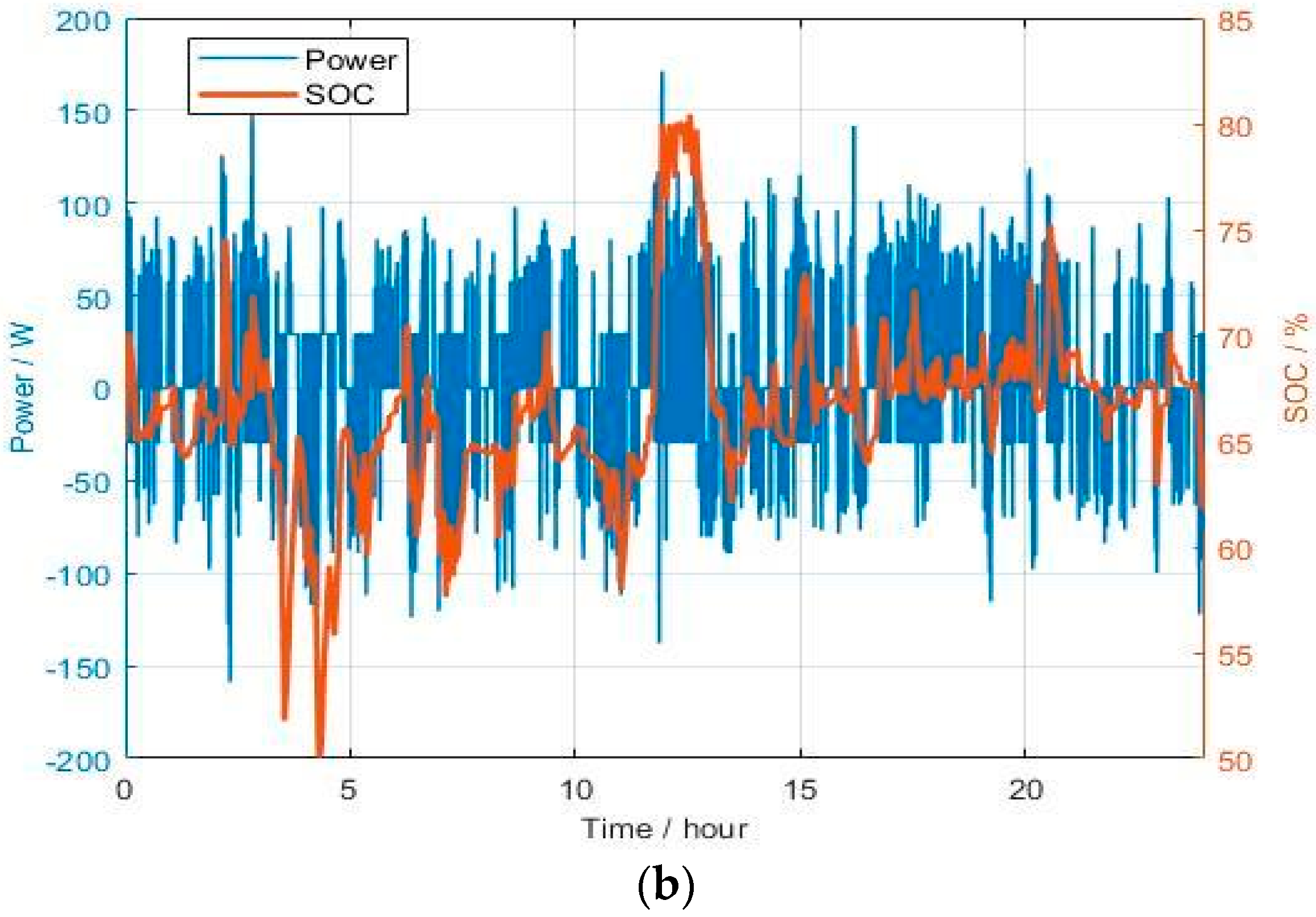
| Parameter | Normal Pattern | Severe Pattern |
|---|---|---|
| Total Energy (Wh) | 229.70 | 493.68 |
| Charge Energy (Wh) | 114.69 | 246.75 |
| Discharge Energy (Wh) | 115.01 | 246.93 |
| Energy for Frequency Regulation “f > 60.03” (Wh) | 96.07 | 185.76 |
| Energy for Frequency Regulation “f < 59.97” (Wh) | 23.40 | 135.00 |
| SOC Recovery Energy “SOC < 63” (Wh) | 18.62 | 60.99 |
| SOC Recovery Energy “SOC > 67” (Wh) | 91.61 | 111.93 |
| Maximum Charge Power (W) | 147.57 | 170.94 |
| Maximum Discharge Power (W) | 98.21 | 158.73 |
| Average Charge C-rate | 0.79 | 0.68 |
| Average Discharge C-rate | 0.45 | 0.59 |
| Maximum SOC (%) | 80.2 | 80.0 |
| Minimum SOC (%) | 61.0 | 50.0 |
© 2019 by the authors. Licensee MDPI, Basel, Switzerland. This article is an open access article distributed under the terms and conditions of the Creative Commons Attribution (CC BY) license (http://creativecommons.org/licenses/by/4.0/).
Share and Cite
Kwon, S.-J.; Kim, G.; Park, J.; Lim, J.-H.; Choi, J.; Kim, J. Research of Adaptive Extended Kalman Filter-Based SOC Estimator for Frequency Regulation ESS. Appl. Sci. 2019, 9, 4274. https://doi.org/10.3390/app9204274
Kwon S-J, Kim G, Park J, Lim J-H, Choi J, Kim J. Research of Adaptive Extended Kalman Filter-Based SOC Estimator for Frequency Regulation ESS. Applied Sciences. 2019; 9(20):4274. https://doi.org/10.3390/app9204274
Chicago/Turabian StyleKwon, Soon-Jong, Gunwoo Kim, Jinhyeong Park, Ji-Hun Lim, Jinhyeok Choi, and Jonghoon Kim. 2019. "Research of Adaptive Extended Kalman Filter-Based SOC Estimator for Frequency Regulation ESS" Applied Sciences 9, no. 20: 4274. https://doi.org/10.3390/app9204274
APA StyleKwon, S.-J., Kim, G., Park, J., Lim, J.-H., Choi, J., & Kim, J. (2019). Research of Adaptive Extended Kalman Filter-Based SOC Estimator for Frequency Regulation ESS. Applied Sciences, 9(20), 4274. https://doi.org/10.3390/app9204274