Abstract
Liquefaction is considered a damaging phenomenon of earthquakes and a major cause of concern in civil engineering. Therefore, its predictory assessment is an essential task for geotechnical experts. This paper investigates the performance of Bayesian belief network (BBN) and C4.5 decision tree (DT) models to evaluate seismic soil liquefaction potential based on the updated and relatively large cone penetration test (CPT) dataset (which includes 251 case histories), comparing them to a simplified procedure and an evolutionary-based approach. The BBN model was developed using the K2 machine learning algorithm and domain knowledge (DK) with data fusion methodology, while the DT model was created using a C4.5 algorithm. This study shows that the BBN model is preferred over the others for evaluation of seismic soil liquefaction potential. Owing to its overall performance, simplicity in practice, data-driven characteristics, and ability to map interactions between variables, the use of a BBN model in assessing seismic soil liquefaction is quite promising. The results of a sensitivity analysis show that ‘equivalent clean sand penetration resistance’ is the most significant factor affecting liquefaction potential. This study also interprets the probabilistic reasoning of the robust BBN model and most probable explanation (MPE) of seismic soil liquefied sites, based on an engineering point of view.
1. Introduction
Liquefaction-induced hazards (for instance, settlements, sand boils, lateral spreading, and ground cracks) cause substantial infrastructure damages to buildings, bridges, and lifelines during earthquakes [1,2,3,4,5]. Thus, it is important to assess the occurrence of soil liquefaction potential and its effects in a seismically active region for earthquake-induced hazard mitigation. Several empirical and semi-empirical methods of liquefaction quantification are presented in the literature [6]. Many of these existing methods are based on correlations between in-situ test measurements and field observation data, and are extensions of the ‘simplified procedure’ developed by Seed and Idriss [7]. The in-situ cone penetration test (CPT) has been used by numerous researchers to evaluate seismic soil liquefaction potential (e.g., Juang et al. [8], Youd et al. [6]). The principal advantage of the CPT is that it offers a continuous record of penetration resistance in soil profiles, which enables more detailed subsurface exploration than other in-situ tests.
Artificial intelligence (AI) techniques—adaptive neuro fuzzy inference system (ANFIS) [9], artificial neural network (ANN) method [10], support vector machine (SVM) [11,12], patient ruled-induction method (PRIM) [13], and stochastic gradient boosting (SGB) [14]—have been successfully applied to seismic soil liquefaction assessment based on an in-situ test database. Nevertheless, most of the introduced AI techniques have the following limitations [14,15,16]: (1) difficulty in concluding the assessment results due to limited use of prior knowledge; (2) trouble in integrating various sources of information into a coherent system; (3) not proficient in assessing uncertainty; and (4) black box nature.
In this paper, Bayesian belief network (BBN) and C4.5 decision tree (DT) approaches are employed to assess seismic soil liquefaction potential based on the updated and relatively large cone penetration test (CPT) database, which includes 251 case histories. BBN is a graphical model that permits a probabilistic association between a set of variables based on the Bayes theorem [17]. There are extended uses of the Bayesian belief network (BBN) in the fields of civil engineering; for example, in seismic hazard assessment [18,19], risk assessment for bridges [19] and buildings [20,21], and diagnosis of embankment dam distress [22,23]. Nevertheless, BBN model applications in seismic soil liquefaction study are still limited [24,25,26]. There is no comprehensive BBN model based on machine learning algorithm (ML) and domain knowledge (DK) data fusion methodology to evaluate soil liquefaction potential based on the CPT database. Decision tree (DT) algorithms, such as interactive dichotomizer version 3 (ID3) [27] and commercial version 4.5 (C4.5) [28], are quite transparent. One of the advantages of DT analysis is that the relationship between the binary dependent variable and the related independent variables is clearly illustrated using a tree structure. Hence, decision trees are well-liked and powerful tools in data mining [29]. Limited research work has been reported in the literature on predicating seismic soil liquefaction. Gandomi et al. [30] used three different DT approaches i.e., chi-squared automatic interaction detection (CHAID), exhaustive CHAID, and classification and regression tree (CART) algorithms for assessment of soil liquefaction. Ardakani and Kohestani [16] used the C4.5 DT model on 109 CPT-based case histories; they considered seven significant factors of seismic soil liquefaction—cone tip resistance (qc), total vertical stress (σv), vertical effective stress (σv′), mean grain size (D50), peak ground acceleration (amax), cyclic stress ratio (τ/σv′), and earthquake magnitude (M)—without paying attention to sampling bias in the training and testing data sets. This study extends the scope of research on this topic by considering extra factors i.e., eleven significant factors of seismic soil liquefaction, and the updated and relatively large dataset of 251 case histories with approximately no sampling bias.
This study is significant in several ways:
- (1)
- The BBN and C4.5 DT effective approaches are used to evaluate and compare the seismic soil liquefaction potential of the updated and relatively large cone penetration test (CPT) data set, which includes 251 case history records. In addition, the developed models are compared with the Youd et al. [6] and Rezania et al. [31] models to validate performance.
- (2)
- One of the major advantages of the presented models is the consideration and addition of earthquake parameters to the dataset—the causative fault type and closest distance to rupture surface parameter.
- (3)
- Data division for training and testing datasets was performed with due attention to statistical aspects, such as minimum, maximum, mean, and standard deviation of the datasets. The splitting of the datasets helped identify the predictive ability and generalization performance of the developed models, and evaluate them better.
- (4)
- This study presents probabilistic reasoning, most probable explanation of seismic soil liquefied sites, and parametric sensitivity analysis of the robust model.
The paper is organized into six main sections. The following section describes the basics of the BBN and C4.5 DT approaches, illustrating the proposed framework for seismic soil liquefaction potential assessment. Section 3 details the development of the BBN and C4.5 decision tree models. Section 4 presents the performance evaluation measures of the proposed approaches. The results are presented in Section 5. Finally, the last section presents a discussion and conclusions, along with ideas for future work.
2. Predictive Modeling Techniques
2.1. Bayesian Belief Network (BBN)
Bayesian belief network (BBN) is a directed acyclic graph (DAG) comprising of a set of variables (nodes), arcs, and conditional probability tables, which indicate joint probability distributions among the nodes of variables. The nodes in BBN can be categorized into two kinds, parent node and child node, as shown in Figure 1.
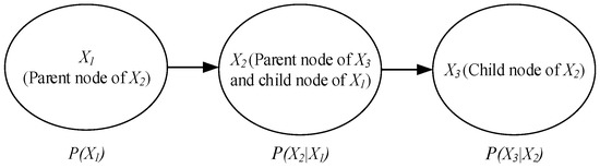
Figure 1.
A simple Bayesian belief network.
One of BBN’s significances is that joint probability distributions can be easily identified. In BBN, if the probability of the variable Xi’s parent nodes is defined as Pa(Xi), joint probability distributions P(X), X = (X1, X2, X3, ..., Xn) can be represented as:
where X = (X1, X2, X3, ..., Xn) expressing various BBN variables, n is the number of BBN variables. Another significance is that the probability can be updated dynamically when there is new evidence. If new evidence (event Y) is provided to BBN, the posterior probability i.e., P(X|Y) of event X is found as:
where marginal probability of event Y is P(Y) and prior probability of event X is P(X).
The construction of a BBN primarily includes two steps: (1) Structure learning determine the factor variables (nodes) related to the study object, and then identify the dependent or independent relationship among the factor variables, so as to develop a DAG structure. (2) Parameter learning is based on the given BBN structure to study the conditional probability table at each variable node.
Effective structure learning is essential in the construction of an optimal BBN network structure. The development of a BBN structure comprises of any one of the following listed three methods:
(1) The variable nodes of a BBN are determined by prior or domain knowledge (DK) and expert experience.
(2) A BBN structure is acquired through learning of sample data, automatically by using a machine learning (ML) algorithm.
(3) A BBN structure is acquired by using data fusion methodology based on DK and ML of data.
Since the third method integrates the strengths of both DK and ML, it eliminates the pitfalls that arise by utilizing only one method. Therefore, this paper uses this method to identify a BBN structure for assessment of seismic soil liquefaction potential. To perform structural learning from a dataset, frequently used ML algorithms, such as K2 and hill-climbing were used. In this study, the K2 algorithm [32] is applied to perform structure learning that carries out a search in accordance with the given order of nodes by means of restricted maximum number of parent nodes. A K2 machine learning algorithm employs posterior probabilities as the scoring function and adds arcs to BBN, which depend on the following rules [32]:
(1) Calculate the Cooper-Herskovits (CH) score for according to the nodes’ order .
where is the number of samples, which are subject to , , , and .
(2) Add an arc , when (i) makes the maximum. are the parents of .
The pseudocode of the K2 algorithm [32] in this study using variables set X = {X1, X2, …, Xn} denotes the nodes of variables, such as depth of soil deposit, groundwater table, fines content, earthquake magnitude, thickness of soil layer, soil behavior type index, equivalent clean sand penetration resistance, liquefaction potential, etc., as shown in Table 1. To acquire an optimal network structure, DK is included in the K2 machine learning algorithm. The proposed BBN structure for liquefaction potential assessment is developed by the K2 machine learning algorithm. It is further fine-tuned based on the domain knowledge (DK) of field experts and known relationships between different input factors.

Table 1.
K2 algorithm pseudocode.
Once the topological structure of the BBN is obtained, parameter learning is performed to identify the conditional probability distribution of each variable node under a given BBN. Three basic kinds of algorithms are thus used: maximum likelihood estimation (MLE), gradient descent (GD), and expectation maximization (EM). The MLE is the fastest and simplest algorithm, based entirely on data and independent of prior probabilities; thus, it does not apply to models containing latent variables and datasets with several missing values [33]. EM and GD algorithms work in an iterative process, but EM is suitable for data that contains missing values. In short, EM learning frequently takes a BBN, uses it to perform a desired (E) step, and then proceeds to maximize (M) to find a better network [34].
2.2. C4.5 Decision Tree (DT) Model
C4.5, introduced by Quinlan [28], is a well-known algorithm, mostly employed for design decision trees. In general, in a decision tree, each branch node depicts a choice among a number of alternatives, and each leaf node denotes a classification or decision. An unknown (or test) instance is routed down the tree as per the values of the attributes in the successive nodes. When the instance reaches a leaf, it is classified as per the label designated to the corresponding leaf.
In the initial step of model construction, a decision-tree induction algorithm is utilized to construct the tree. Numerous algorithms for decision-tree induction exist; they include Interactive dichotomizer version 3 (ID3) [27], commercial version 4.5 (C4.5) [28], and classification and regression tree (CART) [35]. C4.5 and CART are the most widely used decision tree algorithms in literature [36]. Therefore, this study uses the C4.5 decision tree approach to assess seismic soil liquefaction potential. C4.5 algorithm is an extension of the ID3 algorithm and uses the divide-and-conquer technique, whose key improvements incorporate pruning methodology and processing of missing values, numeric attributes, and noisy data [28]. A statistical test used in C4.5 for handling an attribute to each node in the tree also uses an entropy-based measure. The designated tribute is the one with the highest information gain ratio among attributes available at that tree construction point. The information gain ratio (A, S) of an attribute ‘A’ relative to the sample set ‘S’ is represented as:
where
and
where, ‘Sa’ is the subset of ‘S’ for which attribute ‘A’ has value ‘a’. Clearly, the information gain ratio can be obtained directly for discrete-valued attributes.
3. Development of Seismic Soil Liquefaction Modeling
3.1. Dataset, Date Preprocessing, and Predictor Variables
The dataset used in this study is based on an updated version of cone penetration test case history records compiled by Boulanger and Idriss [37]. The dataset consists of 253 cases with soil behavior type index, Ic < 2.6; 180 of them are liquefied cases, 71 are non-liquefied cases, and the remaining 2 are doubtful cases (margin between liquefaction and non-liquefaction), which have been eliminated in this study to reduce epistemic uncertainty (an individual case record can have only one performance outcome—either liquefaction or non-liquefaction). These case history records are derived from CPT measurements at sites and field performance observations of 17 different earthquakes—7 in the United States of America, 4 in New Zealand, 3 in Japan, and 1 each in China, Taiwan, and Turkey. Readers can refer to Boulanger and Idriss [37] for details of the CPT case histories.
Soil liquefaction is influenced by seismic parameters, soil properties, and site geometry conditions that contain a diversified set of factors. Previous studies [25,26,38,39,40,41] offer a detailed understanding of the process, leading to appropriate selection of variables, discretization, and classification in this study. Therefore, 11 influence factors or variables—earthquake magnitude (M), peak ground acceleration (amax, g), closest distance to rupture surface, (rrup, km), fines content (Fc, %), equivalent clean sand penetration resistance (qc1Ncs), soil behavior type index (Ic), vertical effective stress (σ’v, kPa), total vertical stress, (σv, kPa), groundwater table depth (Dw, m), depth of soil deposit (Ds, m), and thickness of soil layer (Ts, m)—are used for evaluation of liquefaction potential. The new earthquake factor i.e., closest distance to rupture surface, (rrup), was estimated through an attenuation equation derived by Sadigh et al. [42]; it considers the influence of an earthquake’s causative fault type and the effect of an earthquake near a fault zone. It has a range of 4 to 8+ for earthquake magnitude (M) and up to 100 km for closest distance to rupture surface, (rrup); in this paper, it is proposed for use for a maximum earthquake magnitude (M) of 9 with a range of 1 to 107.03 km for closest distance to rupture surface, (rrup).
A BBN has a strong ability to deal with discrete variables, albeit weak in processing with continuous variables. The K2 machine learning (ML) algorithm, meanwhile, requires variables to be discrete; thus, it is necessary to convert the 11 influence factors into discrete values before building the BBN models. The liquefaction potential (output) was given a binary value of 0 for non-liquefied sites and a value of 1 for liquefied sites. Table 2 presents the grading standards for seismic soil liquefaction factors.
Table 2.
Grading standards for seismic soil liquefaction factors.
To construct the models, the dataset was divided into two data subsets:
- A training dataset is required to train the models. In this research work, the authors used 80% of the data i.e., 201 out of 251 CPT case histories are considered for the training set.
- A testing dataset is needed to predict the developed models’ performance. In this study, the remaining 20% of data i.e., 50 out of 251 CPT case histories are considered as the testing dataset.
Data division for training and testing datasets was performed with due attention to statistical aspects, such as minimum, maximum, mean, and standard deviation of the datasets. The statistical consistency of the training and testing datasets optimizes the models’ performance and subsequently assists in evaluating them better. The statistical parameters of the input variables include the minimum, maximum, mean, and standard deviation of the training and testing datasets; they are shown in Table 3. Splitting of the dataset helps identify the generalization performance and predictive ability of the developed models. Similar performance of both training and testing datasets demonstrates that the developed models may be applied for the trained ranges. As is indicated in Table 3, input and output parameters for testing ranges exist in training datasets.
Table 3.
Descriptive statistics of variables used in the model training and testing dataset.
3.2. Model Development Using BBNs
A BBN structure is developed by using data fusion methodology based on an ML algorithm i.e., K2 learning from CPT case histories using FullBNT-1.0.7 tool in MATLAB, following which effective information is embedded as DK (deleting direct links of depth of soil deposit and thickness of soil layer to liquefaction potential) (see Figure 2). Consequently, the new BBN comprises of two separate networks as the thickness of soil layer has no relation to the other nodes, implying that the thickness of soil layer can be detached from the model. Thus, the network is composed of 11 nodes and several lines. The lines among these nodes represent the relationships. It can be seen from Figure 2 that soil liquefaction variables have counter-intuitive results by means of dependence. For example, “peak ground acceleration” is dependent on “earthquake magnitude”, “closest distance to rupture surface”, and others.
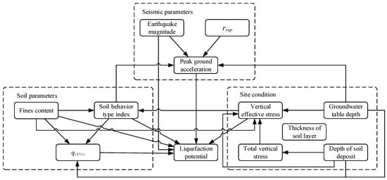
Figure 2.
A Bayesian belief network (BBN) structure for seismic soil liquefaction potential based on the K2 machine learning (ML) algorithm and domain knowledge (DK).
The network structure is created in Netica free version software (distributed by Norsys Software Corporation (https://www.norsys.com/) under Norsys License Agreement) to acquire conditional probability distribution of the nodes via parameter learning. Ultimately, a Bayesian belief network model was created to assess seismic soil “liquefaction potential”, as shown in Figure 3.
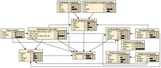
Figure 3.
Graphical result of a BBN-based seismic soil liquefaction potential model using K2 and DK.
3.3. Model Development Using C4.5 Decision Tree
To build the model, a C4.5 DT algorithm was implemented using Waikato Environment for Knowledge Analysis (WEKA) software, which is open source and freely available. The WEKA workbench is a collection of state-of-the-art ML algorithms and data-preprocessing tools. The dataset in attribute relation file format (ARFF) is loaded in WEKA to train the C4.5 DT model. The C4.5 DT model is then tested by providing a testing dataset based on the given training set. The decision tree of seismic soil liquefaction potential using a C4.5 algorithm is shown in Figure 4.
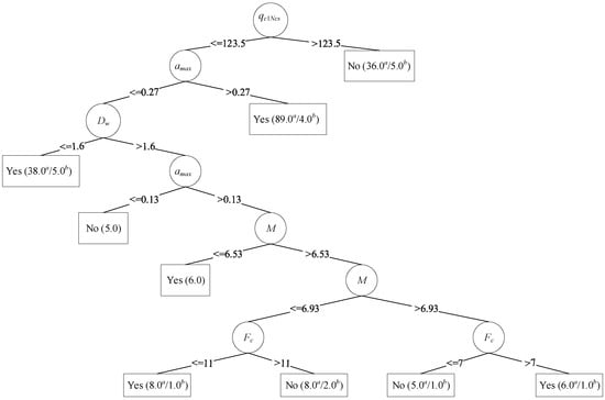
Figure 4.
Decision tree of seismic soil liquefaction generated by a C4.5 algorithm. a Number of cases in this partition; b Number of cases misclassified.
4. Performance Measure
The performances of the proposed models were evaluated by a number of metrics, identified using a confusion matrix for proper comparison (Table 4).
Table 4.
Confusion matrix.
The definitions of key terminology used to formulate the elementary metrics while considering the non-occurrence of liquefaction is actually negative class are:
- True positive (TP) and true negative (TN) indicate that the samples are predicted correctly.
- False positive (FP) represents the number of non-liquefied samples that are predicted incorrectly as positive.
- False negative (FN) denotes the number of liquefied samples that are predicted incorrectly as negative.
- Precision refers to the accuracy of the predictions for a single class (positive or negative).
- Recall measures the accuracy of predictions, considering only the predicted value.
Based on the confusion matrix, the following metrics were used to evaluate and compare the prediction models:
Data on seismic soil liquefaction case histories usually exhibit class imbalances, wherein one event i.e., liquefaction, in this case, is delineated by a large number of events, while non-liquefaction event is presented by scarcely any. Therefore, overall accuracy (OA) may be deceptive—it has high scores when the liquefied samples are in the majority class. In this study, one of the standard measures used is the Matthews correlation coefficient (MCC) [43]. MCC presents the degree of correlation between the actual and predicted classes of liquefied and non-liquefied instances. MCC takes values in the interval [−1,1], with “1” showing complete agreement, “−1” complete disagreement, and “0” presenting that the prediction was uncorrelated with the ground truth. The MCC value is regarded to be the best evaluation measure for overall performance of a classifier method [44]. F-measure combines precision and recall values to attain a harmonic mean. F-measure ranges from 0 (worst value) to 1 (best value). The receiver operating characteristic (ROC) curve is a graphic plot of the sensitivity or recall against false positive rate (FPR). The FPR is given by:
The ROC curve gives a comprehensive scalar value that describes the expected performance of the model. The area under curve (AUC) is employed to summarize the ROC curve. The ROC curve has five degrees of rating [45]: excellent (0.9–1), good (0.8–0.9), fair (0.7–0.8), poor (0.6–0.7), and not discriminating (0.5–0.6).
Concisely, a model with good OA, larger AUC, high F-measure, and high MCC is an ideal one.
5. Results
5.1. Comparative Performance of Training and Testing Datasets
Performance comparison of BBN models were made for training and testing datasets. The ratio of the number of liquefied case history records to non-liquefied case history records is 2.53:1 for the training dataset. It is obvious that there is a class imbalance problem. The ratio for testing and total datasets is 2.57:1 and 2.54:1, respectively, which indicates that there is approximately no sampling bias in the training and testing datasets. The BBN and C4.5 DT models were developed from the training dataset of 201 CPT case histories (144 case records of liquefaction and 57 case records of non-liquefaction) that has class imbalances and almost no sampling bias owing to the class ratio of 180:71 for 251 case histories.
Table 5 shows that the BBN model has a higher OA, while OA alone cannot be utilized as a model performance measure; therefore, AUC of ROC, MCC, precision, recall, and F-measure were also used to select optimal model performance separately for liquefaction and non-liquefaction instances. For liquefaction, the BBN model has a higher recall, whereas the C4.5 DT model has maximum precision. However, when F-measure is computed, the BBN model has a highest value and moreover has the highest value of AUC and MCC, with respect to the C4.5 DT model. In the case of the non-liquefaction class the BBN model has a higher precision value, while the C4.5 DT model has a high recall value; however, the F-measure for BBN has higher value. BBN has shown to have a relatively good OA, MCC, AUC, and F-measure for liquefaction and non-liquefaction instances, offering better performance.
Table 5.
Performance evaluation of the training dataset.
The predictive performance of the BBN and C4.5 DT models are compared with the Youd et al. [6] simplified procedure, referred to as CPT-YD; and the Rezania et al. evolutionary-based approach [31], referred to as CPT-RA, with the same testing dataset (36 case records of liquefaction and 14 case records of non-liquefaction). Table 6 clearly shows that BBN has the highest OA, AUC, and MCC. In the case of liquefaction and non-liquefaction classes, BBN has the highest scores in all parameters, barring one (the C4.5 DT model has the highest value of recall in the liquefaction class). The BBN model, thus, showed robust performance in comparison with C4.5 DT, CPT-YD, and CPT-RA.
Table 6.
Predictive performance evaluation of the testing dataset.
5.2. Analysis of a Robust BBN Model
5.2.1. Probabilistic Reasoning
The developed robust BBN may be employed to perform probability reasoning, which includes calculations of posterior probability-sequential inference (from causes to results) and causal inference-reverse inference (from results to causes).
(I) Liquefaction Potential Prediction
Liquefaction potential prediction is shown in Figure 5 on the basis of the supposition that peak ground acceleration is “medium”, groundwater table depth is “shallow”, and soil behavior type index grade is “silty sand or sand with silt”. On fixing these parameters as 100% in Netica, the state of the evidence variables is identified. Subsequently, the probabilities of a robust BBN model are updated; and the probability change of “liquefaction potential” and the remaining variable nodes are noted. In this instance, the “yes” state probability in “liquefaction potential” is identified to scale up from 58.2% to 63.6%. This indicates that when peak ground acceleration is “medium”, groundwater table depth is “shallow”, and soil behavior type index grade is “silty sand or sand with silt”, the liquefaction potential probability of the “yes” state will notably increase (see Figure 5).
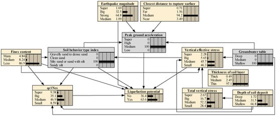
Figure 5.
Liquefaction potential prediction when the states of evidence variables are: “PGA = medium,” “Dw = shallow,” and “Ic = silty sand or sand with silt.”
As shown in Figure 6, in addition to “medium” peak ground acceleration, “shallow” groundwater table depth, and “silty sand or sand with silt” soil behavior type index, it was assumed that the depth of soil deposit status is “shallow” and the status of “medium” in “equivalent clean sand penetration resistance” is 100%. Thereafter, automatically updating the probabilities of robust BBN, the liquefaction potential probability of “yes” is found to further increase from 63.6% to 79.6%, which means that the liquefaction potential probability of “yes” status is higher with respect to the initial probability of 58.2%. This suggests that “peak ground acceleration”, “groundwater table”, “soil behavior type index”, “equivalent clean sand penetration resistance”, and “depth of soil deposit” will affect the liquefaction potential probability of the “yes” state to varying extents. It is to be noted that the change in state of the evidence node variables affects the probability of objective nodes, which is compatible with engineering judgment.
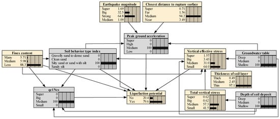
Figure 6.
Liquefaction potential prediction when the state of evidence variables are “PGA = medium,” “Dw = shallow,” “Ic = silty sand or sand with silt,” “qc1Nc s = medium,” and “Ds = shallow.”
(II) Causal Inference
The most significant utilization of the BBN model is to find system faults using its diagnostic reasoning capability; for example, by carrying out causal inference and selecting the evidence state “yes” in “liquefaction potential”. Here, the evidence state is “yes”; therefore, the probability is 100%. As illustrated in Figure 7, after fixing the evidence “yes”, the probability of “medium” in “peak ground acceleration” and “silty sand or sand with silt” in soil behavior type index increases from 45.8% to 47.0% and 71.8% to 76.4%, respectively, using Netica’s automatic updating function. The “shallow” state in “groundwater table” and “depth of soil deposit” probability also increases from 62.7% to 63.4% and 66.7% to 67.1%, respectively. This recommends that, in the absence of remaining evidences, the most likely causes of “liquefaction potential” to the “yes” state are the “shallow” states of “groundwater table” and “depth of soil deposit”, and “medium” grade of peak ground acceleration and “silty sand or sand with silt” class of soil behavior type index.
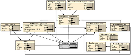
Figure 7.
Posterior probability when the liquefaction potential evidence state is “yes.”
5.2.2. Most Probable Explanation
The most probable explanation (MPE) can be drawn using a function in Netica, which perceives which scenario is most likely to provide a cause set of liquefaction potential. The developed BBN model may be utilized to derive the most probable explanation. For example, if the liquefaction potential state is “yes” (as presented in Figure 8), the “most probable explanation” function is used to provide the most likely cause set of “liquefaction potential”, which, in this case, is: earthquake magnitude = strong, peak ground acceleration = medium, closest distance to rupture surface=medium, fines content = less, soil behavior type index = silty sand or silt with sand, qc1Ncs = medium, vertical effective stress = small, total vertical stress = small, groundwater table depth = shallow, and depth of soil deposit = shallow. This clearly shows that the most probable explanation set is considerably compatible and well matched with engineering judgment.
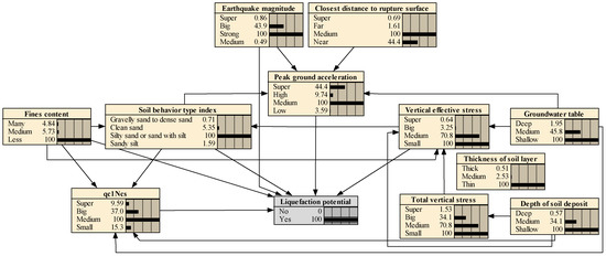
Figure 8.
The most probable explanation of liquefaction potential when the evidence state is “yes.”
5.2.3. Sensitivity Analysis
The literature offers large and diverse information on sensitivity analysis—how each factor affects the uncertainty of the target variable. For instance, Hamdia et al. [46] carried out a sensitivity analysis to determine the key input parameters impacting the relation between tissue structure and mechanics. Ayad et al. [47] performed a sensitivity analysis and showed that soil’s parameter variability has a significant effect on soil liquefaction probability.
In BBN, sensitivity analysis refers to the influence each variable has on the uncertainty of target nodes. In Netica, a function of sensitivity analysis is utilized to identify the factors that have a great influence on liquefaction potential. The target node “liquefaction potential” is selected for the sensitivity analysis; the results are presented in Table 7.
Table 7.
Sensitivity analysis of “liquefaction potential”.
The mutual information of two nodes may show interdependency and correlation [48]. Table 7 highlights that mutual information of the “equivalent clean sand penetration resistance” node is the greatest (0.022310, which shows that it has the strongest influence on “liquefaction potential”), followed by “soil behavior type index,” “peak ground acceleration,” “vertical effective stress,” and “fines content,” with values of 0.010800, 0.004560, 0.003450, and 0.002980, respectively. These results are highly compatible with those in the literature.
6. Discussion and Conclusions
In a BBN, the input of expert knowledge can enable the realistic integration of domain knowledge with statistical data. In addition, all the parameters in a BBN have an understandable semantic interpretation. Furthermore, a BBN model can always be updated as new data become available. The authors in this study selected 11 direct significant variables or factors of seismic soil liquefaction, while other researchers (e.g., Ardakani and Kohestani [16]) used indirect parameters i.e., cyclic stress ratio (CSR). In the proposed BBN models, soil, seismic, and site condition factors are encoded directly from a CPT dataset, instead of just cyclic resistance ratio (CRR) and CSR; this can be effectively utilized by geotechnical professionals to evaluate seismic soil liquefaction potential. No calibration or normalization of cone tip resistance, qc (MPa), was done in previous studies (e.g., Ardakani and Kohestani [16], Tesfamariam and Liu [49], Goh and Goh [5]). However, in this work, qc1Ncs, the equivalent clean sand penetration resistance, was used to decrease uncertainty. Additionally, Pirhadi et al. [50] concluded that normalized cone tip penetration value (qc1N) is an important factor, and has the highest effect on seismic soil liquefaction triggering.
The resulting BBN model showed a relatively better performance for training and testing data than other models for the metrics of overall accuracy (OA), MCC, precision, recall and F-measure, and AUC of ROC. The limitations of the proposed robust BBN are: too much reliance on bulk data and not being suitable for missing values, owing to the learning demands of the K2 ML algorithm.
Discerning earthquake-induced soil liquefaction is a complicated and nonlinear procedure, affected by diversified factors of uncertainties. In this paper, two effective approaches—BBN and C4.5 DT—are presented to examine the seismic soil liquefaction potential assessment. They are then compared with a simplified procedure and an evolutionary-based approach. The major findings in this study are presented as follows:
- The BBN model has relatively better results, as compared to the C4.5 DT, CPT-YD, and CPT-RA models. Considering its overall predictive accuracy, MCC, precision, recall, F-measure for liquefaction and non-liquefaction instances, AUC of ROC, simplicity in practice, data-driven characteristics, and the ability to map interactions between variables, the use of the BBN model in evaluating seismic soil liquefaction by multiple complex factors is quite promising.
- The proposed robust BBN model can not only quantitatively predict seismic soil liquefaction potential probability under certain influence factors (seismic, soil, and site conditions), but also identify the main diagnostic reasons and fault-finding states’ combinations presumed to support decisions on seismic soil liquefaction mitigation measures for sustainable development.
- The sensitivity analysis results conclude that “equivalent clean sand penetration resistance”, “soil behavior type index’, “groundwater table”, “peak ground acceleration’, “vertical effective stress”, and “fines content” are the most sensitive factors in descending order in the assessment of liquefaction potential, and are well matched with the literature.
- The “most probable explanation” function is used to provide the most likely cause set of seismic soil liquefied sites, which is: earthquake magnitude = strong, peak ground acceleration = medium, closest distance to rupture surface = medium, fines content = less, soil behavior type index = silty sand or silt with sand, qc1Ncs = medium, vertical effective stress = small, total vertical stress = small, groundwater table depth = shallow, and depth of soil deposit = shallow. This is considerably compatible and well matched with engineering judgment.
In future, the following points need to be addressed as an extension of this work:
- The BBN model can be used to assess vulnerability of land damage resulting from seismic soil liquefaction by adding nodes of liquefaction land damage potential.
- Additional CPT case history records should be collected and an attempt made to avoid class imbalance in the dataset (caused by updating the BBN model’s conditional probability table) and improve the performance results of prediction.
- The nodes of ‘utility’ and ‘decision operations’ should be added to seismic soil liquefaction and the BBN’s land damage potential model, which can eventually be used as important decision-making information in case of expected utility of loss.
Author Contributions
Conceptualization, X.-W.T. and J.-N.Q.; methodology, J.-N.Q. and X.-W.T.; software, M.A.; validation, M.A.; formal analysis, M.A.; investigation, X.-W.T. and M.A.; resources, M.A.; data curation, M.A. and F.A.; writing—original draft preparation, M.A.; writing—review and editing, M.A. and F.A.; visualization, M.A.; supervision, X.-W.T. and J.-N.Q.; project administration, X.-W.T.; funding acquisition, X.-W.T.
Funding
This paper was part of a research work sponsored by the National Key Research & Development Plan of China (Grant No. 2018YFC1505300-5.3 and 2016YFE0200100) and Key Program of National Natural Science Foundation of China (Grant No. 51639002).
Acknowledgments
The authors extend their gratitude to Ji-Lei Hu and Kuang Chang, among other experts, for their opinion on building of the BBN.
Conflicts of Interest
The authors declare no conflict of interest.
References
- Oommen, T.; Baise, L.G.; Vogel, R. Validation and Application of Empirical Liquefaction Models. J. Geotech. Geoenviron. Eng. 2010, 136, 1618–1633. [Google Scholar] [CrossRef]
- Tang, X.-W.; Bai, X.; Hu, J.-L.; Qiu, J.-N. Assessment of liquefaction-induced hazards using Bayesian networks based on standard penetration test data. Nat. Hazards Earth Syst. Sci. 2018, 18, 1451–1468. [Google Scholar] [CrossRef]
- Kohestani, V.R.; Hassanlourad, M.; Ardakani, A. Evaluation of liquefaction potential based on CPT data using random forest. Nat. Hazards 2015, 79, 1079–1089. [Google Scholar] [CrossRef]
- Wang, Z.; Zhao, D.; Liu, X.; Chen, C.; Li, X. P and S wave attenuation tomography of the Japan subduction zone. Geochem. Geophys. Geosyst. 2017, 18, 1688–1710. [Google Scholar] [CrossRef]
- Goh, A.T.; Goh, S. Support vector machines: Their use in geotechnical engineering as illustrated using seismic liquefaction data. Comput. Geotech. 2007, 34, 410–421. [Google Scholar] [CrossRef]
- Youd, T.L.; Idriss, I.M. Liquefaction resistance of soils: Summary report from the 1996 NCEER and 1998 NCEER/NSF workshops on evaluation of liquefaction resistance of soils. J. Geotech. Geoenviron. Eng. 2001, 127, 297–313. [Google Scholar] [CrossRef]
- Seed, H.B.; Idriss, I.M. Simplified procedure for evaluating soil liquefaction potential. J. Soil Mech. Found. Div. 1971, 97, 1249–1273. [Google Scholar]
- Juang, C.H.; Yuan, H.; Lee, D.-H.; Lin, P.-S. Simplified Cone Penetration Test-based Method for Evaluating Liquefaction Resistance of Soils. J. Geotech. Geoenviron. Eng. 2003, 129, 66–80. [Google Scholar] [CrossRef]
- Xue, X.; Yang, X. Application of the adaptive neuro-fuzzy inference system for prediction of soil liquefaction. Nat. Hazards 2013, 67, 901–917. [Google Scholar] [CrossRef]
- Goh, A.T.C. Neural-Network Modeling of CPT Seismic Liquefaction Data. J. Geotech. Eng. 1996, 122, 70–73. [Google Scholar] [CrossRef]
- Samui, P. Seismic liquefaction potential assessment by using Relevance Vector Machine. Earthq. Eng. Eng. Vib. 2007, 6, 331–336. [Google Scholar] [CrossRef]
- Pal, M. Support vector machines-based modelling of seismic liquefaction potential. Int. J. Numer. Anal. Methods Géoméch. 2006, 30, 983–996. [Google Scholar] [CrossRef]
- Kaveh, A.; Hamze-Ziabari, S.M.; Bakhshpoori, T. Patient rule-induction method for liquefaction potential assessment based on CPT data. Bull. Int. Assoc. Eng. Geol. 2016, 77, 849–865. [Google Scholar] [CrossRef]
- Zhou, J.; Li, E.; Wang, M.; Chen, X.; Shi, X.; Jiang, L. Feasibility of Stochastic Gradient Boosting Approach for Evaluating Seismic Liquefaction Potential Based on SPT and CPT Case Histories. J. Perform. Constr. Facil. 2019, 33, 04019024. [Google Scholar] [CrossRef]
- Liang, W.-J.; Zhuang, D.-F.; Jiang, D.; Pan, J.-J.; Ren, H.-Y. Assessment of debris flow hazards using a Bayesian Network. Geomorphology 2012, 171, 94–100. [Google Scholar] [CrossRef]
- Ardakani, A.; Kohestani, V.R. Evaluation of liquefaction potential based on CPT results using C4.5 decision tree. J. Artif. Intell. Data Min. 2015, 3, 85–92. [Google Scholar]
- Pearl, J. Probabilistic Reasoning in Intelligent Systems; Morgan Kaufmann Publishers: San Mateo, CA, USA, 1988. [Google Scholar]
- Bayraktarli, Y.Y.; Baker, J.W.; Faber, M.H. Uncertainty treatment in earthquake modelling using Bayesian probabilistic networks. Georisk Assess. Manag. Risk Eng. Syst. Geohazards 2011, 5, 44–58. [Google Scholar] [CrossRef]
- Bensi, M.T.; Der, K.A.; Straub, D. A Bayesian Network framework for post–earthquake infrastructure system performance assessment. In Proceedings of the TCLEE 2009: Lifeline Earthquake Engineering in a Multi-hazard Environment, Oakland, CA, USA, 28 June–1 July 2009. [Google Scholar]
- Bayraktarli, Y.Y.; Faber, M.H. Bayesian probabilistic network approach for managing earthquake risks of cities. Georisk Assess. Manag. Risk Eng. Syst. Geohazards 2011, 5, 2–24. [Google Scholar] [CrossRef]
- Faizian, M.; Schalcher, H.R.; Faber, M.H. Consequence assessment in earthquake risk management using damage indicators. In Proceedings of the 9th International Conference on Structural Safety and Reliability (ICOSSAR 05), Rome, Italy, 19–23 June 2005; pp. 19–23. [Google Scholar]
- Jia, J.; Zhang, L.; Xu, Y.; Zhao, C. Diagnosis of embankment dam distresses using Bayesian networks. Part I. Global-level characteristics based on a dam distress database. Can. Geotech. J. 2011, 48, 1630–1644. [Google Scholar]
- Jia, J.; Xu, Y.; Zhang, L. Diagnosis of embankment dam distresses using Bayesian networks. Part II. Diagnosis of a specific distressed dam. Can. Geotech. J. 2011, 48, 1645–1657. [Google Scholar]
- Bayraktarli, Y.Y. Application of Bayesian probabilistic networks for liquefaction of soil. In Proceedings of the 6th International PhD Symposium in Civil Engineering, Zurich, Switzerland, 23–26 August 2006. [Google Scholar]
- Hu, J.-L.; Tang, X.-W.; Qiu, J.-N. A Bayesian network approach for predicting seismic liquefaction based on interpretive structural modeling. Georisk Assess. Manag. Risk Eng. Syst. Geohazards 2015, 9, 200–217. [Google Scholar] [CrossRef]
- Hu, J.-L.; Tang, X.-W.; Qiu, J.-N. Assessment of seismic liquefaction potential based on Bayesian network constructed from domain knowledge and history data. Soil Dyn. Earthq. Eng. 2016, 89, 49–60. [Google Scholar] [CrossRef]
- Quinlan, J.R. Induction of decision trees. Mach. Learn. 1986, 1, 81–106. [Google Scholar] [CrossRef]
- Quinlan, J.R. C4.5: Programs for Machine Learning; Morgan Kaufmann: San Francisco, CA, USA, 1993. [Google Scholar]
- Duch, W.; Setiono, R.; Zurada, J. Computational intelligence methods for rule-based data understanding. Proc. IEEE 2004, 92, 771–805. [Google Scholar] [CrossRef]
- Gandomi, A.H.; Fridline, M.M.; Roke, D.A. Decision Tree Approach for Soil Liquefaction Assessment. Sci. World J. 2013, 2013, 1–8. [Google Scholar] [CrossRef]
- Rezania, M.; Faramarzi, A.; Javadi, A.A. An evolutionary based approach for assessment of earthquake-induced soil liquefaction and lateral displacement. Eng. Appl. Artif. Intell. 2011, 24, 142–153. [Google Scholar] [CrossRef]
- Cooper, G.F.; Herskovits, E. A Bayesian Method for the Induction of Probabilistic Networks from Data. Mach. Learn. 1992, 9, 309–347. [Google Scholar] [CrossRef]
- Spiegelhalter, D.J.; Lauritzen, S.L. Sequential updating of conditional probabilities on directed graphical structures. Networks 1990, 20, 579–605. [Google Scholar] [CrossRef]
- Lauritzen, S.L. The EM algorithm for graphical association models with missing data. Comput. Stat. Data Anal. 1995, 19, 191–201. [Google Scholar] [CrossRef]
- Breiman, L.; Friedman, J.; Olshen, R.; Stone, C. Classification and Regression Trees; Wadsworth International Group: San Francisco, CA, USA, 1984. [Google Scholar]
- Mesarić, J.; Šebalj, D. Decision trees for predicting the academic success of students. Croat. Oper. Res. Rev. 2016, 7, 367–388. [Google Scholar] [CrossRef]
- Boulanger, R.; Idriss, I. CPT and SPT Based Liquefaction Triggering Procedures; Report No. UCD/CGM–14/01; Center for Geotechnical Modeling, Department of Civil and Environmental Engineering, University of California: Davis, CA, USA, 2014. [Google Scholar]
- Tranfield, D.; Denyer, D.; Smart, P. Knowledge by Means of Systematic Review. Br. J. Manag. 2003, 14, 207–222. [Google Scholar] [CrossRef]
- Okoli, C.; Schabram, K. A Guide to Conducting a Systematic Literature Review of Information Systems Research. Working Papers on Information Systems. SSRN Electron. J. 2010, 10, 1–51. [Google Scholar]
- Zhang, L.Y. Predicting Seismic Liquefaction Potential of Sands by Optimum Seeking Method. Soil Dyn. Earthq. Eng. 1998, 17, 219–226. [Google Scholar] [CrossRef]
- Ahmad, M.; Tang, X.-W.; Qiu, J.-N.; Ahmad, F. Interpretive Structural Modeling and MICMAC Analysis for Identifying and Benchmarking Significant Factors of Seismic Soil Liquefaction. Appl. Sci. 2019, 9, 233. [Google Scholar] [CrossRef]
- Sadigh, K.; Chang, C.-Y.; Egan, J.A.; Makdisi, F.; Youngs, R.R. Attenuation Relationships for Shallow Crustal Earthquakes Based on California Strong Motion Data. Seism. Res. Lett. 1997, 68, 180–189. [Google Scholar] [CrossRef]
- Matthews, B. Comparison of the predicted and observed secondary structure of T4 phage lysozyme. Biochim. Biophys. Acta (BBA)-Protein Struct. 1975, 405, 442–451. [Google Scholar] [CrossRef]
- Baldi, P.; Brunak, S.; Chauvin, Y.; Andersen, C.A.F.; Nielsen, H. Assessing the accuracy of prediction algorithms for classification: An overview. Bioinformatics 2000, 16, 412–424. [Google Scholar] [CrossRef]
- Bradley, A.P. The use of the area under the ROC curve in the evaluation of machine learning algorithms. Pattern Recognit. 1997, 30, 1145–1159. [Google Scholar] [CrossRef]
- Hamdia, K.M.; Marino, M.; Zhuang, X.; Wriggers, P.; Rabczuk, T. Sensitivity analysis for the mechanics of tendons and ligaments: Investigation on the effects of collagen structural properties via a multiscale modeling approach. Int. J. Numer. Methods Biomed. Eng. 2019, 35, e3209. [Google Scholar] [CrossRef]
- Ayad, F.; Abdelmalek, B.; Youcef, H. Sensitivity Analysis of Soil Liquefaction Potential. Earth Sci. Res. 2014, 3, 14–24. [Google Scholar] [CrossRef]
- Cheng, J.; Greiner, R.; Kelly, J.; Bell, D.; Liu, W. Learning Bayesian networks from data: An information-theory based approach. Artif. Intell. 2002, 137, 43–90. [Google Scholar] [CrossRef]
- Tesfamariam, S.; Liu, Z. Seismic risk analysis using Bayesian belief networks. In Handbook of Seismic Risk Analysis and Management of Civil Infrastructure Systems; Woodhead Publishing: Cambridge, UK, 2013; pp. 175–208. [Google Scholar]
- Pirhadi, N.; Tang, X.; Yang, Q.; Kang, F. A New Equation to Evaluate Liquefaction Triggering Using the Response Surface Method and Parametric Sensitivity Analysis. Sustainability 2018, 11, 112. [Google Scholar] [CrossRef]


© 2019 by the authors. Licensee MDPI, Basel, Switzerland. This article is an open access article distributed under the terms and conditions of the Creative Commons Attribution (CC BY) license (http://creativecommons.org/licenses/by/4.0/).