Dependency Model-Based Multiple Fault Diagnosis Using Knowledge of Test Result and Fault Prior Probability

Abstract

Aiming at solving the multiple fault diagnosis problem as well as the sequence of all the potential multiple faults simultaneously, a new multiple fault diagnosis method based on the dependency model method as well as the knowledge in test results and the prior probability of each fault type is proposed. Firstly, the dependency model of the system can be built and used to formulate the fault-test dependency matrix. Then, the dependency matrix is simplified according to the knowledge in the test results of the system. After that, the logic ‘OR’ operation is performed on the feature vectors of the fault status in the simplified dependency matrix to formulate the multiple fault dependency matrix. Finally, fault diagnosis is based on the multiple fault dependency matrix and the ranking of each fault type calculated basing on the prior probability of each fault status. An illustrative numerical example and a case study are presented to verify the effectiveness and superiority of the proposed method.

1. Introduction

Fault diagnosis is the basis of the maintenance work for complex equipment and systems, such as the components in an aircraft [1,2], a motor [3,4,5], a diesel engine [6], and so on [7]. In practical applications, multiple fault states may exist in a complex system, while various available tests can be applied for fault detection [8,9,10]. How to locate the potential multiple faults for further maintenance work is an important issue [11]. Because of the complexity of the system under test, it is not easy to build a mathematical model for a complex system. Thus, the method based on a signal flow model, which is mainly based on the information flow of the system, is popular among researchers for theoretical research and practical applications [12,13]. After analyzing and building the signal flow graphs model of a complex system, the dependency model can be generated for the following fault diagnosis and maintenance work.

The dependency model is a promising method to analyze the correlation between the tests and the possible failures in the equipment [14]. In general, dependency model-based fault diagnosis methods can be divided into two categories:

• The sequential diagnosis method [15,16,17,18]: Sequential diagnosis is a kind of testing and diagnosis method basing on a cycle process of “test–diagnosis–retest”. The sequential diagnosis method is especially suitable for a system which is at the phase of principle testing and prototype developing. To obtain the correct diagnosis results with the minimum test cost, an optimal test sequence in the diagnosis strategy should be constructed, which is a typical NP (Non-deterministic Polynomial)-complete problem. Currently, more research focuses on the hypotheses of single fault and reliable test results to reduce the hardship of solving the problem.
• Concurrent fault diagnosis method [19,20,21]: The concurrent fault diagnosis method is a traditional monitoring diagnosis method, where all the tests are completed before applying the diagnosis procedure. The whole diagnosis process only needs one cycle of testing and diagnosis procedure. Since it requires all the symptoms or at least most of the symptoms in advance to gain the correct diagnosis results, the concurrent fault diagnosis method is more suitable for a system where abundant sensing information can be acquired. A typical method for concurrent diagnosis is that the fault prior probability of the components in the system is known, the posterior probability of each component can be calculated and the maximum posteriori probability will be used to determine the corresponding fault component. The limitation of this method is that it only searches for one optimal solution and the suboptimal solution will be abandoned, which may easily fall into the local optimum.

To address the multiple fault diagnosis problem as well as the sequence of all the potential multiple faults simultaneously, a new simple dependency model-based fault diagnosis method is proposed in this paper. The two-valued logic, where both the fault and the test have only two Boolean logic values of 0 or 1, is adopted to address the problem, which means the dependency relation is a certain correlation. The proposed method is different from the fuzzy logic-based method [22,23,24], where the fuzzy logic mainly focuses on an uncertain or fuzzy correlation, which is represented by the membership function. The two-valued logic can describe a certain correlation between a fault and a test. The knowledge included in the test results is applied to formulate the fault ambiguity group, including multiple fault types in the system, while the prior probability of each fault type will be used to calculate the ranking of the potential fault types in the fault ambiguity group. An illustrative experiment and a case study are applied to verify the effectiveness of the proposed method.

This rest of this paper is organized as follows. The problem formulation is introduced in Section 2. In Section 3, a new multiple fault diagnosis method is proposed. Then, an illustrative experiment and a case study are presented in Section 4 and Section 5, respectively, to verify the proposed. Section 6 draws the conclusions of this paper.

2. Problem Formulation

Assuming that m (m = 1, 2, 3, ...) fault states exist in a system while n (n = 1, 2, 3, ...) tests are designed for the system, the dependency model-based multiple fault diagnosis problem can be formulated as follows:

$$\Re =\left\{F,P,T,FT,R\right\},$$

(1)

where

$$\left\{\begin{array}{c}F=\left\{f_1,\cdots ,f_m\right\},\hfill \\ P=\left\{p\left(f_1\right),\cdots ,p\left(f_m\right)\right\},\hfill \\ T=\left\{t_1,t_2,\cdots ,t_n\right\},\hfill \\ FT={\left[f{t}_{ij}\right]}_{m\times n},\hfill \\ R=\left\{r_1,r_2,\cdots ,r_n\right\}.\hfill \end{array}\right.$$

(2)

All the parameters in Equations (1) and (2) are interpreted as follows:

• F means the set of independent fault states in the system. $f_l$$\left(1\le l\le m\right)$ represents the lst fault state;
• P means the set of the prior probability among all the fault states that happens independently; $p\left(f_i\right)$$\left(1\le i\le m\right)$ represents the prior probability of the fault $f_i$ happens alone;
• T means a finite set consisting of all the available tests in the system. Here, assume that each test result is reliable with an output in the form of a binary number;
• $FT$ represents the dependency matrix of fault test results, of which the expression is defined as follows:

  $$FT={\left[\begin{array}{cccc}f{t}_{11}& f{t}_{12}& \cdots & f{t}_{1n}\\ f{t}_{21}& f{t}_{22}& \cdots & f{t}_{2n}\\ ⋮& ⋮& \cdots & ⋮\\ f{t}_{m1}& f{t}_{m2}& \cdots & f{t}_{mn}\end{array}\right]}_{m\times n}.$$

  (3)

  $FT$ is a matrix with a scale of $m\times n$. The element $f{t}_{ij}$ denotes the correlation between a fault state $f_i$ in F and a test $t_j$ in T. If $f{t}_{ij}=1$, then the fault state $f_i$ can be tested by the test $t_j$. If $f{t}_{ij}=0$, then the test $t_j$ fails to know the situation about the fault state $f_i$. In this way, in Equation (3), the rows in the matrix $FT$ denote the set of fault types, while the columns denote the set of tests;
• R is a set of the observation results according to the tests in the system, e.g., $r_1$ is the observation result of the test $t_1$. For each test $t_n$, the corresponding observation result $r_n$ will be only one of the following two states:

  –

  ‘Pass’, denoted by ‘0’. The system passes the test;

  –

  ‘Fail’, denoted by ‘1’. The system fails to pass the test.

In summary, to solve the dependency model-based multiple fault diagnosis problem is to locate a suspicious set of fault $X\subset F$ based on the fault-test dependency matrix $FT$, the prior probability set of the fault states P and the set of the observation results R in a system. After that, all the fault states in the suspicious set X will be ranked according to the priority in which each fault may happen, which will be based on the prior probability. The following maintenance work of a system will be accomplished based on the rankings of the fault states.

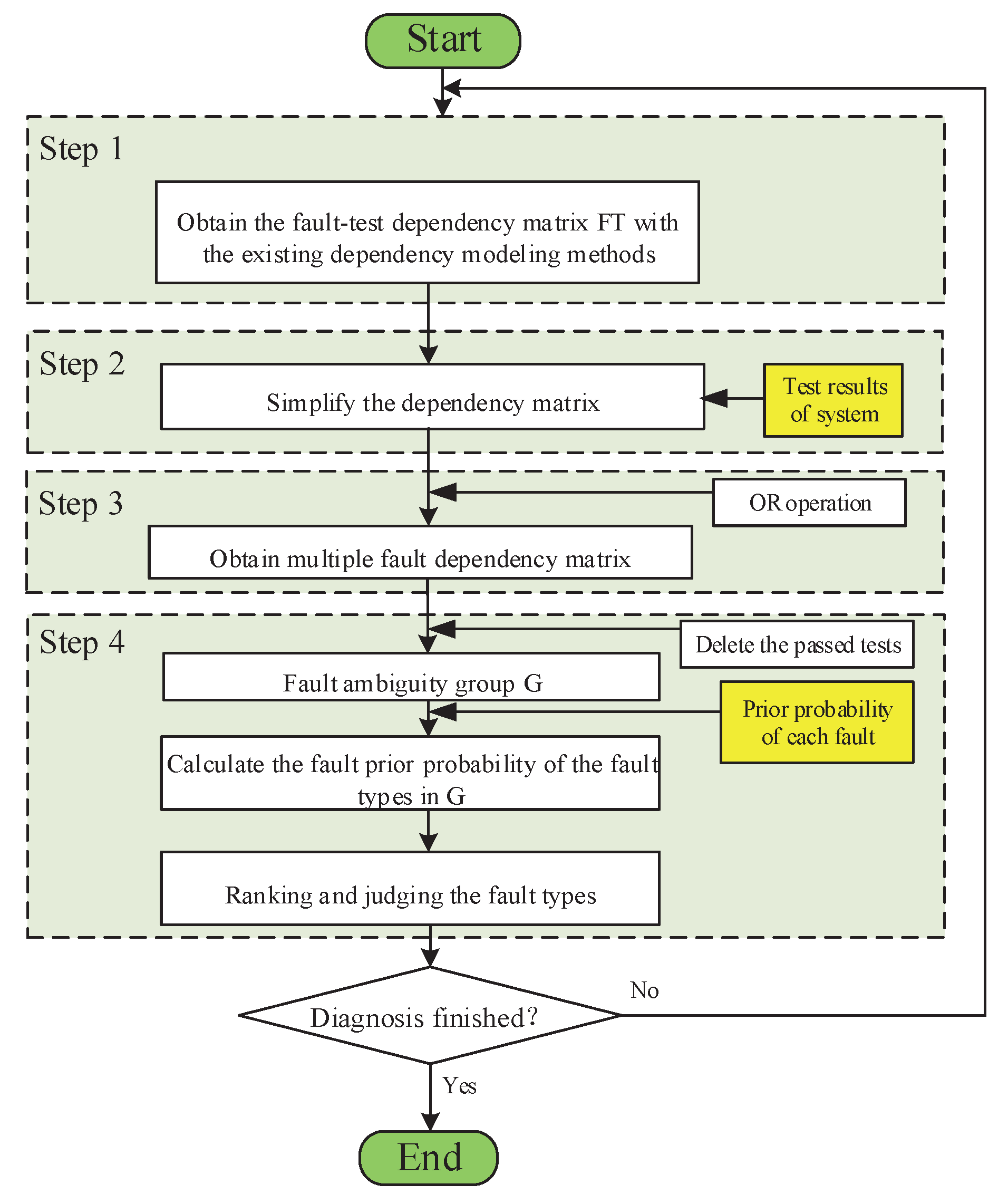
3. A New Multiple Fault Diagnosis Method

The implementation process of the proposed multiple fault diagnosis method based on the test results and the prior probability of each fault types is presented in Figure 1.

In general, four steps are included in the proposed method, designed and explained as follows.

• Step 1. Build the fault-test dependency matrix based on the existing dependency modeling methods. Analyze the system and build its dependency model based on the information flows or the multisignal flow graphs model [12,25]. After that, the dependency matrix in the form of Equation (3) can be built based on the reachability algorithm [26] or experimental design method [21,27].
• Step 2. Simplify the dependency matrix $FT$ according to the test results of the system. The purpose of this step is to delete the impossible fault states according to the test results. For example, if $f{t}_{ij}=1$, which means the test $t_j$ is correlated with the fault type $f_i$ and the test result of $t_j$ is ‘Pass’ according to the observation result ${\mathrm{r}}_j=0$, then the fault type $f_i$ will definitely not happen. In this way, the logical judgment from experts or engineers is applied for simplifying the complex fault diagnosis processing. This can be regarded as a semisupervised diagnosis method.
  In detail, the principle of simplifying the dependency matrix based on the correlation between the test $t_j$ and the fault type $f_i$ can be analyzed as follows.
  • For the element $f{t}_{ij}=1$ in the dependency matrix, which means the test $t_j$ is correlated with the fault type $f_i$, the following cases may exist:

    –

    If the fault $f_i$ happens, the result of the test $t_j$ must be ‘1’ (Fail);

    –

    If the fault $f_i$ does not happen, the result of the test $t_j$ is unknown;

    –

    If the result of the test $t_j$ is ‘1’ (Fail), the state of the fault $f_i$ is unknown; in this case, $t_j$ may be caused by $f_i$ or the other fault like $f_k$;

    –

    If the result of the test $t_j$ is ‘0’ (Pass), the fault type $f_i$ will not happen.

  • For the element $f{t}_{ij}=0$ in the dependency matrix, which means the test $t_j$ is not correlated with the fault type $f_i$, the following cases may exist:

    –

    If the fault $f_i$ happens, the result of the test $t_j$ is unknown because there is no correlation between $t_j$ and $f_i$;

    –

    If the fault $f_i$ does not happen, the result of the test $t_j$ is unknown, too;

    –

    If the result of the test $t_j$ is ‘1’ (Fail), the state of the fault $f_i$ is unknown;

    –

    If the result of the test $t_j$ is ‘0’ (Pass), the state of the fault $f_i$ is unknown.

  After analyzing the cases in the correlation between the test $t_j$ and the fault type $f_i$, the method of simplifying the dependency matrix $FT$ can be concluded as follows:
  • Delete the column vectors correlated to the test result $t_j=0$ (‘Pass’ the test) in the dependency matrix $FT$. Only the items correlated to the test $t_j=1$ (‘Fail’ to pass the test) are reserved.
  • Delete the row vectors correlated to $f{t}_{ij}=1$ in the column that satisfies $t_j=0$.
  Finally, the simplified matrix $F{T}_y={\left[f{t}_{ij}\right]}_{h\times k}$ can be formulated where $1\le h\le m$, $1\le k\le n$.
• Step 3. Formulate the multiple fault dependency matrix $F{T}_d$ by logic operation. Perform the logical ‘OR’ operation on each fault eigenvector (the row vector) in the simplified matrix $F{T}_y={\left[f{t}_{ij}\right]}_{h\times k}$ to obtain the multiple fault dependency matrix $F{T}_d$. Define that the fault type of single faults is included in the ones of the multiple faults. Thus, the results of the ‘OR’ operation among each fault type vector in the matrix $F{T}_y$ can be used to denote the state in which that multiple fault happens. For example, when the eigenvector of the fault $f_i$ and $f_j$ are $\left[\begin{array}{ccc}0& 1& 0\end{array}\right]$ and $\left[\begin{array}{ccc}1& 0& 0\end{array}\right]$, respectively, then the corresponding eigenvector of the multiple fault is $f_{\left(i,j\right)}$ is $f_{\left(i,j\right)}=f_i∥f_j=\left[\begin{array}{ccc}1& 1& 0\end{array}\right]$. The results of the logic operation ware added at the bottom of the matrix $F{T}_y$ as the new row vectors. Finally, the new matrix are defined as the multiple fault dependency matrix $F{T}_d$, in which the number of the column vector is k and the maximum of the row vector is $2^h-1$.
• Step 4. Fault diagnosis based on the multiple fault dependency matrix $F{T}_d$. If the fault state $f_i$ happens, then all the tests corresponding to the element ‘1’ in the row vector fail. If the chosen tests all fail, then the row vectors in the matrix $FT$ correlated to the fault $f_i$ are all ‘1’. Therefore, if the row vectors in the matrix $FT$ correlated to the fault $f_i$ include the element ‘0’, then delete the corresponding rows where the element ‘0’ is included in. Now, the remaining fault states, in which the elements in the row vector are all ‘1’, are the suspicious fault types. All the suspicious fault types constitute the fault ambiguity group denoted as G.
  Ranking all the suspicious fault types in the fault ambiguity group G based on the fault prior probability, where the prior probability of the multiple fault type $f_{\left(i,j\right)}$ generated in the third step can be calculated as follows:

  $$p\left(f_{\left(i,j\right)}\right)=p\left(f_i\right)\times p\left(f_j\right).$$

  (4)
  Actions such as fault isolation or removal in the system will be based on the ranking results of the fault types.

The fault diagnosis process is finished once the fault has been successfully located and removed, or the whole procedure is applied again in the system.

4. Illustrative Experiment

As an illustrative experiment, the dependency model-based multiple fault diagnosis method is applied to a control system. The dependency model of the control system is shown as Figure 2. Apart from the common fault $f_1$, two branches are included in the model: (1) The first branch includes the faults $f_2$ and $f_3$, (2) the second branch includes the fault $f_4$.

In Figure 2, each fault state $f_i$ (i = 1, 2, 3.) in the dependency model can be tested according to the corresponding test $t_i$ along to the arrow. The results of some cases are obvious and definite, e.g.,

• If the fault $f_1$ happens, the observation results of all the tests including $t_1$, $t_2$, $t_3$ and $t_4$ must be ‘Fail’;
• If the fault $f_4$ happens, the observation result of the test $t_4$ is definitely ‘Fail’.

In the control system, the prior probability of each fault state is as follows: $p\left(f_1\right)=0.1$, $p\left(f_2\right)=0.2$, $p\left(f_3\right)=0.3$, and $p\left(f_4\right)=0.4$. Assume that the test result of each fault according to the observation result in the system is as follows: $t_1=r_1=0$ (‘Pass’), $t_2=r_2=1$ (‘Fail’), $t_3=r_3=1$ (‘Fail’), and $t_4=r_4=1$ (‘Fail’).

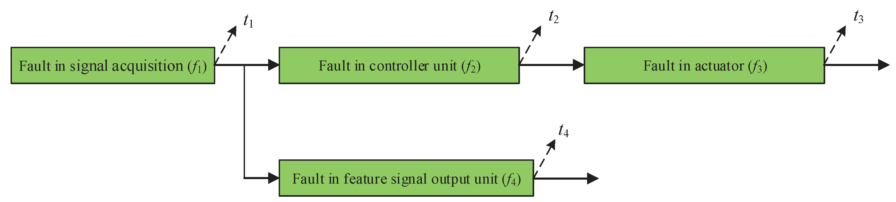
4.1. Experiment Process

Step 1: Build the dependency model of the system to obtain the dependency matrix. Build the fault-test dependency matrix of the control system based on the reachability algorithm [26]. The aforementioned control system is not that complex; its fault-test dependency matrix is formulated as

Table 1. Fault-test dependency matrix of the control system.

Fault Type	${\mathit{t}}_1$	${\mathit{t}}_2$	${\mathit{t}}_3$	${\mathit{t}}_4$
Signal collector fault $f_1$	1	1	1	1
Controller unit fault $f_2$	0	1	1	0
Actuator fault $f_3$	0	0	1	0
Feature signal output unit fault $f_4$	0	0	0	1

. In Figure 2 and Table 1, $t_1$, $t_2$, $t_3$, and $t_4$ denote 4 independent tests, while $f_1$, $f_2$, $f_3$, and $f_4$ denote 4 independent fault types. In detail, the 4 independent tests and the 4 fault types are shown as follows:

• $t_1$ denotes a signal acquisition test,
• $t_2$ denotes a controller unit efficiency test,
• $t_3$ denotes an actuator action range test,
• $t_4$ denotes a feature signal output test,
• $f_1$ denotes a signal collector fault,
• $f_2$ denotes a controller unit fault,
• $f_3$ denotes an actuator fault, and
• $f_4$ denotes a feature signal output unit fault.

Step 2: Simplify the dependency matrix according to the test results of the system. The system only ‘Pass’ the test $t_1$ according to the observation results of the test, where $t_1=0$, $t_2=1$, $t_3=1$, and $t_4=1$. According to the dependency model in Table 1, among all the column vectors correlated to the test $t_1$, only $f{t}_{11}=1$, which means only $f_1$ is correlated to $t_1$ ($f{t}_{21}=f{t}_{31}=f{t}_{41}=0$); thus, the fault type $f_1$ cannot be wrong. Delete the column vector corresponding to $t_1$ and the row vector corresponding to $f_1$ to get the simplified dependency matrix is shown in

Table 2. Simplified dependency matrix of the control system.

Fault Type	${\mathit{t}}_2$	${\mathit{t}}_3$	${\mathit{t}}_4$
Controller unit fault $f_2$	1	1	0
Actuator fault $f_3$	0	1	0
Feature signal output unit fault $f_4$	0	0	1

.

Step 3: Formulate the multiple fault dependency matrix. Perform the logical OR operation on the eigenvector (the row vector) of each fault type based on the simplified dependency matrix presented in Table 2. The eigenvector of multiple faults can be formulated as follows:

• Fault in Controller and Actuator unit $f_{\left(2,3\right)}$.
  $f_{\left(2,3\right)}=f_2∥f_3=\left[110\right]∥\left[010\right]=\left[110\right]$.
• Fault in Controller and Feature signal output unit $f_{\left(2,4\right)}$.
  $f_{\left(2,4\right)}=f_2∥f_4=\left[110\right]∥\left[001\right]=\left[111\right]$.
• Fault in Actuator and Feature signal output unit $f_{\left(3,4\right)}$.
  $f_{\left(3,4\right)}=f_3∥f_4=\left[010\right]∥\left[001\right]=\left[011\right]$.
• Fault in Controller unit, Actuator and Feature signal output unit $f_{\left(2,3,4\right)}$.
  $f_{\left(2,3,4\right)}=f_2∥f_3∥f_4=\left[110\right]∥\left[010\right]∥\left[001\right]=\left[111\right]$.

The multiple fault dependency matrix is formulated as

Table 3. Multiple fault dependency matrix of the system.

Fault Type	${\mathit{t}}_2$	${\mathit{t}}_3$	${\mathit{t}}_4$
Controller unit fault $f_2$	1	1	0
Actuator fault $f_3$	0	1	0
Feature signal output unit fault $f_4$	0	0	1
Fault in Controller and Actuator unit $f_{\left(2,3\right)}$	1	1	0
Fault in Controller and Feature signal output unit $f_{\left(2,4\right)}$	1	1	1
Fault in Actuator and Feature signal output unit $f_{\left(3,4\right)}$	0	1	1
Fault in Controller, Actuator and Feature signal output unit $f_{\left(2,3,4\right)}$	1	1	1

.

Step 4: Fault diagnosis of the system based on the multiple fault dependency matrix. For the multiple fault dependency matrix shown in Table 3, delete the row vector of the fault type with ‘0’ including $f_2$, $f_3$, $f_4$, $f_{\left(2,3\right)}$, and $f_{\left(2,3,4\right)}$. After that, the the fault ambiguity group G can be formulated, as shown in

Table 4. Fault ambiguity group of the control system.

Fault Type	${\mathit{t}}_2$	${\mathit{t}}_3$	${\mathit{t}}_4$
Controller unit and Feature signal output unit fault $f_{\left(2,4\right)}$	1	1	1
Controller unit, Actuator and Feature signal output unit fault $f_{\left(2,3,4\right)}$	1	1	1

.

Calculating the prior probability of the multiple fault in the fault ambiguity group G, the result is as follows:

$$p\left(f_{\left(2,4\right)}\right)=p\left(f_2\right)\times p\left(f_4\right)=0.2\times 0.4=0.08,$$

$$\begin{array}{c}p\left(f_{\left(2,3,4\right)}\right)=p\left(f_2\right)\times p\left(f_3\right)\times p\left(f_4\right)=0.2\times 0.3\times 0.4=0.024.\hfill \end{array}$$

It is easy to know that $p\left(f_{\left(2,4\right)}\right)>p\left(f_{\left(2,3,4\right)}\right)$ according to the calculation result, which means that the possibility of the fault in the Controller and the Feature output unit $f_{\left(2,4\right)}$ is greater than that of the Controller, Actuator, and Feature signal output unit $f_{\left(2,3,4\right)}$.

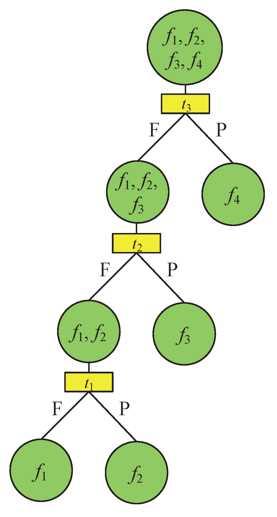
4.2. A Simple Discussion in Comparison With Diagnosis Tree

In comparison with the diagnosis tree method, the proposed method can successfully locate the multiple fault types.

With the optimal design method based on the diagnostic strategy in sequential diagnosis, the fault-diagnosis tree is shown as Figure 3.

Since the test result of the system is $t_1=0$, $t_2=1$, $t_3=1$, and $t_4=1$, the diagnosis conclusion is that the fault type $f_2$ fails based on the fault-diagnosis tree of the system. It is not the correct diagnosis conclusion that $f_2$ is the fault type because the fault status may also exist in another fault unit, like $f_3$, $f_4$, or the aforementioned fault types simultaneously. The proposed method is able to locate the fault with a fault ambiguity group G, including $f_{\left(2,4\right)}$ and $f_{\left(2,3,4\right)}$. In addition, the proposed method gives a probability on the fault diagnosis result which shows that the possibility that the fault $f_{\left(2,4\right)}$ happens is greater than that of $f_{\left(2,3,4\right)}$. Above all, the proposed method provides a basis of decision-making for the diagnosis and maintenance of the control system.

5. A Case Study

The test matrix of fault isolation in the Apollo Manned Lunar Landing program was adopted for the case study [28]. The original dependency matrix of the case study is shown in

Table 5. Dependency matrix for fault diagnosis adopted from the Apollo system [28].

Fault Type	${\mathit{T}}_1$	${\mathit{T}}_2$	${\mathit{T}}_3$	${\mathit{T}}_4$	${\mathit{T}}_5$	${\mathit{T}}_6$	${\mathit{T}}_7$	${\mathit{T}}_8$	${\mathit{T}}_9$	${\mathit{T}}_{10}$	${\mathit{T}}_{11}$	${\mathit{T}}_{12}$	${\mathit{T}}_{13}$	${\mathit{T}}_{14}$	${\mathit{T}}_{15}$
$F_1$	0	0	0	1	0	0	0	1	0	1	1	1	1	0	0
$F_2$	0	0	1	0	1	0	0	0	0	0	1	1	0	1	0
$F_3$	0	0	0	0	1	1	1	0	1	1	1	1	0	0	1
$F_4$	0	1	0	0	0	1	1	0	0	0	0	0	0	1	1
$F_5$	0	1	0	1	0	1	1	1	1	1	0	0	1	1	0
$F_6$	0	0	0	1	1	0	0	1	1	1	0	1	1	1	1
$F_7$	1	0	0	1	1	0	0	0	0	0	0	1	0	1	1
$F_8$	1	1	1	0	0	1	1	0	1	1	1	0	0	1	0
$F_9$	1	0	0	1	1	0	0	0	0	0	0	1	0	1	1
$F_{10}$	1	1	1	1	0	0	1	0	0	0	1	0	1	1	0

.

5.1. Experiment 1

Assume that (1) the prior probability of each failure is 0.1, and (2) the tests $T_1$, $T_3$, and $T_{11}$ are passed (denoted as ‘Pass’, 0), all the other tests have failed (denoted as ‘Fail’, 1). Perform the proposed method on this case.

5.1.1. Experiment Process

Step 1: Build the fault-test dependency matrix. The dependency matrix is adopted from the literature [28] and presented in Table 5.

Step 2: Simplify the dependency matrix according to the test results of the system. The test results of the system are: $T_1$ = 0, $T_3$ = 0, $T_{11}$ = 0; $T_2$, $T_4$, $T_5$, $T_6$, $T_7$, $T_8$, $T_9$, $T_{10}$, $T_{12}$, $T_{13}$, $T_{14}$, and $T_{15}$ are all equal to 1. Thus, it can be concluded that the test results of $T_1$, $T_3$, and $T_{11}$ are qualified and no failure will happen in the correlated fault types $F_1$, $F_2$, $F_3$, $F_7$, $F_8$, $F_9$, and $T_{10}$. Thus, the simplified matrix can be formulated and shown in

Table 6. Simplified dependency matrix of the case study in Experiment 1.

Fault Type	${\mathit{T}}_2$	${\mathit{T}}_4$	${\mathit{T}}_5$	${\mathit{T}}_6$	${\mathit{T}}_7$	${\mathit{T}}_8$	${\mathit{T}}_9$	${\mathit{T}}_{10}$	${\mathit{T}}_{12}$	${\mathit{T}}_{13}$	${\mathit{T}}_{14}$	${\mathit{T}}_{15}$
$F_4$	1	0	0	1	1	0	0	0	0	0	1	1
$F_5$	1	1	0	1	1	1	1	1	0	1	1	0
$F_6$	0	1	1	0	0	1	1	1	1	1	1	1

.

Delete the tests $T_6$, $T_7$, $T_8$, $T_9$, $T_{10}$, $T_{12}$, and $T_{13}$; because of that, (1) $T_6$ and $T_7$ are redundant with $T_2$, and (2) $T_8$, $T_9$, $T_{10}$, and $T_{13}$ are redundant with $T_4$. Thus, the simplified matrix of the system can be formulated, as shown in

Table 7. Simplified dependency matrix of the case study in Experiment 1 after redundancy reduction.

Fault Type	${\mathit{T}}_2$	${\mathit{T}}_4$	${\mathit{T}}_5$	${\mathit{T}}_{14}$	${\mathit{T}}_{15}$
$F_4$	1	0	0	1	1
$F_5$	1	1	0	1	0
$F_6$	0	1	1	1	1

.

Step 3: Formulate the multiple fault dependency matrix. Based on the simplified dependency matrix in Table 7, perform the logical OR operation on the eigenvectors (row vectors) of the fault to obtain the eigenvectors of the multiple fault group, as shown in

Table 8. Multiple fault dependency matrix of the system in Experiment 1.

Fault Type	${\mathit{T}}_2$	${\mathit{T}}_4$	${\mathit{T}}_5$	${\mathit{T}}_{14}$	${\mathit{T}}_{15}$	Prior Probability
$F_4$	1	0	0	1	1	0.1
$F_5$	1	1	0	1	0	0.1
$F_6$	0	1	1	1	1	0.1
$F_{(4,5)}$	1	1	0	1	1	0.01
$F_{(4,6)}$	1	1	1	1	1	0.01
$F_{(5,6)}$	1	1	1	1	1	0.01
$F_{(4,5,6)}$	1	1	1	1	1	0.001

.

Step 4: Fault diagnosis of the system based on the multiple fault dependency matrix. For the multiple fault dependency matrix shown in Table 8, delete the row vector of the fault type with ‘0’, including $F_4$, $F_5$, $F_6$, and $F_{\left(4,5\right)}$. After that, the fault ambiguity group can be formulated, as shown in

Table 9. Fault fuzzy groups of the system in Experiment 1.

Fault Type	${\mathit{T}}_2$	${\mathit{T}}_4$	${\mathit{T}}_5$	${\mathit{T}}_{14}$	${\mathit{T}}_{15}$	Prior Probability
$F_{(4,6)}$	1	1	1	1	1	0.01
$F_{(5,6)}$	1	1	1	1	1	0.01
$F_{(4,5,6)}$	1	1	1	1	1	0.001

.

Calculating the prior probability of the multiple fault in the fault ambiguity group, the result is as follows:

$$p\left(f_{\left(4,5\right)}\right)=p\left(f_4\right)\times p\left(f_5\right)=0.1\times 0.1=0.01,$$

$$p\left(f_{\left(4,6\right)}\right)=p\left(f_4\right)\times p\left(f_6\right)=0.1\times 0.1=0.01,$$

$$p\left(f_{\left(4,5,6\right)}\right)=p\left(f_4\right)\times p\left(f_5\right)\times p\left(f_6\right)=0.1\times 0.1\times 0.1=0.001.$$

According to the calculation results, there are three possible reasons for the system failure, which are $F_{(4,6)}$, $F_{(5,6)}$ or $F_{(4,5,6)}$. In addition, the ranking of the possible failures based on the calculation results of the prior probability is: $F_{(4,6)}=F_{(5,6)}\succ F_{(4,5,6)}$, where “≻” denotes a higher priority.

5.1.2. A Discussion

In order to present the rationality and some superiorities of the proposed method, the experiment results of the case study were compared with some other methods.

• Compare the experiment results with the hypothesis of a single fault. For the system under test where $T_1$, $T_3$, and $T_{11}$ are successfully passed and the rest of the tests are unqualified, if there is a single fault assumption, according to the diagnosis logic, the system will have no solution— while with the proposed method, the fault status can be located on $F_{(4,6)}$, $F_{(5,6)}$ or $F_{(4,5,6)}$, with a possibility suggestion of each diagnosis result for reference.
• Compare the experiment results with the method in the literature [29]. The method in Reference [29] shows that if the fault prior probability and the test results are known, the multiple fault diagnosis can be achieved through the criterion of maximum posterior probability. Although the method is effective, sometimes the result can be insufficient, because it only gives one diagnosis result ($F_{(4,6)}$ in this case study), while the failure may exist in other fault types according to the proposed method.

5.2. Experiment 2

Assume that (1) the prior probability of each failure is 0.1, and (2) the tests $T_4$, $T_8$, and $T_{13}$ are passed (denoted as ‘Pass’, 0), all the other tests fail (denoted as ‘Fail’, 1). Perform the proposed method on this case.

Step 1: Build the fault-test dependency matrix. The dependency matrix is adopted from the literature [28] and presented in Table 5.

Step 2: Simplify the dependency matrix according to the test results of the system. The test results of the system are: $T_4$ = 0, $T_8$ = 0, $T_{13}$ = 0; $T_1$, $T_2$, $T_3$, $T_5$, $T_6$, $T_7$, $T_9$, $T_{10}$, $T_{11}$, $T_{12}$, $T_{14}$, and $T_{15}$ are all equal to 1. Thus, it can be concluded that the test results of $T_4$, $T_8$ and $T_{13}$ are qualified and no failure will happen in the correlated fault types $F_1$, $F_5$, $F_6$, $F_7$, $F_9$, and $T_{10}$. Thus, the simplified matrix can be formulated and shown in

Table 10. Simplified dependency matrix of the case study in Experiment 2.

Fault Type	${\mathit{T}}_1$	${\mathit{T}}_2$	${\mathit{T}}_3$	${\mathit{T}}_4$	${\mathit{T}}_5$	${\mathit{T}}_6$	${\mathit{T}}_7$	${\mathit{T}}_8$	${\mathit{T}}_9$	${\mathit{T}}_{10}$	${\mathit{T}}_{11}$	${\mathit{T}}_{12}$	${\mathit{T}}_{13}$	${\mathit{T}}_{14}$	${\mathit{T}}_{15}$
$F_2$	0	0	1	0	1	0	0	0	0	0	1	1	0	1	0
$F_3$	0	0	0	0	1	1	1	0	1	1	1	1	0	0	1
$F_4$	0	1	0	0	0	1	1	0	0	0	0	0	0	1	1
$F_8$	1	1	1	0	0	1	1	0	1	1	1	0	0	1	0

.

Delete the tests $T_4$, $T_7$, $T_8$, $T_{10}$, $T_{12}$, and $T_{13}$; because of that, (1) $T_5$ is redundant with $T_{12}$, (2) $T_6$ is redundant with $T_7$, and (3) $T_9$ is redundant with $T_{10}$. Thus, the simplified matrix of the system can be formulated, as shown in

Table 11. Simplified dependency matrix of the case study after redundancy reduction in Experiment 2.

Fault Type	${\mathit{T}}_1$	${\mathit{T}}_2$	${\mathit{T}}_3$	${\mathit{T}}_5$	${\mathit{T}}_6$	${\mathit{T}}_9$	${\mathit{T}}_{11}$	${\mathit{T}}_{14}$	${\mathit{T}}_{15}$
$F_2$	0	0	1	1	0	0	1	1	0
$F_3$	0	0	0	1	1	1	1	0	1
$F_4$	0	1	0	0	1	0	0	1	1
$F_8$	1	1	1	0	1	1	1	1	0

.

Step 3: Formulate the multiple fault dependency matrix. Based on the simplified dependency matrix in Table 11, perform the logical OR operation on the eigenvectors (row vectors) of the fault to obtain the eigenvectors of the multiple fault group, as shown in

Table 12. Multiple fault dependency matrix of the system in Experiment 2.

Fault Type	${\mathit{T}}_1$	${\mathit{T}}_2$	${\mathit{T}}_3$	${\mathit{T}}_5$	${\mathit{T}}_6$	${\mathit{T}}_9$	${\mathit{T}}_{11}$	${\mathit{T}}_{14}$	${\mathit{T}}_{15}$
$F_2$	0	0	1	1	0	0	1	1	0
$F_3$	0	0	0	1	1	1	1	0	1
$F_4$	0	1	0	0	1	0	0	1	1
$F_8$	1	1	1	0	1	1	1	1	0
$F_{2,3}$	0	0	1	1	1	1	1	1	1
$F_{2,4}$	0	1	1	1	1	0	1	1	1
$F_{2,8}$	1	1	1	1	1	1	1	1	0
$F_{3,4}$	0	1	0	1	1	1	1	1	1
$F_{3,8}$	1	1	1	1	1	1	1	1	1
$F_{4,8}$	1	1	1	0	1	1	1	1	1
$F_{2,3,4}$	0	1	1	1	1	1	1	1	1
$F_{2,3,8}$	1	1	1	1	1	1	1	1	1
$F_{2,4,8}$	1	1	1	1	1	1	1	1	1
$F_{3,4,8}$	1	1	1	1	1	1	1	1	1
$F_{2,3,4,8}$	1	1	1	1	1	1	1	1	1

.

Step 4: Fault diagnosis of the system based on the multiple fault dependency matrix. For the multiple fault dependency matrix shown in Table 12, delete the row vector of the fault type with ‘0’, including $F_2$, $F_3$, $F_4$, $F_8$, $F_{\left(2,3\right)}$, $F_{\left(2,4\right)}$, $F_{\left(2,8\right)}$, $F_{\left(3,4\right)}$, $F_{\left(4,8\right)}$, and $F_{\left(2,3,4\right)}$. After that, the fault ambiguity group can be formulated, as shown in

Table 13. Fault fuzzy groups of the system in Experiment 2.

Fault Type	${\mathit{T}}_1$	${\mathit{T}}_2$	${\mathit{T}}_3$	${\mathit{T}}_5$	${\mathit{T}}_6$	${\mathit{T}}_9$	${\mathit{T}}_{11}$	${\mathit{T}}_{14}$	${\mathit{T}}_{15}$	Prior Probability
$F_{3,8}$	1	1	1	1	1	1	1	1	1	0.01
$F_{2,3,8}$	1	1	1	1	1	1	1	1	1	0.001
$F_{2,4,8}$	1	1	1	1	1	1	1	1	1	0.001
$F_{3,4,8}$	1	1	1	1	1	1	1	1	1	0.001
$F_{2,3,4,8}$	1	1	1	1	1	1	1	1	1	0.0001

.

Calculating the prior probability of the multiple fault in the fault ambiguity group, the result is as follows:

$$p\left(f_{\left(3,8\right)}\right)=p\left(f_3\right)\times p\left(f_8\right)=0.1\times 0.1=0.01,$$

$$p\left(f_{\left(2,3,8\right)}\right)=p\left(f_2\right)\times p\left(f_3\right)\times p\left(f_8\right)=0.1\times 0.1\times 0.1=0.001,$$

$$p\left(f_{\left(2,4,8\right)}\right)=p\left(f_2\right)\times p\left(f_4\right)\times p\left(f_8\right)=0.1\times 0.1\times 0.1=0.001,$$

$$p\left(f_{\left(3,4,8\right)}\right)=p\left(f_3\right)\times p\left(f_4\right)\times p\left(f_8\right)=0.1\times 0.1\times 0.1=0.001,$$

$$p\left(f_{\left(2,3,4,8\right)}\right)=p\left(f_2\right)\times p\left(f_3\right)\times p\left(f_4\right)\times p\left(f_8\right)=0.1\times 0.1\times 0.1\times 0.1=0.0001.$$

According to the calculation results, there are 5 possible reasons for the system failure, which are $F_{(3,8)}$, $F_{(2,3,8)}$, $F_{(2,4,8)}$, $F_{(3,4,8)}$ or $F_{(2,3,4,8)}$. In addition, the ranking of the possible failures based on the calculation results of the prior probability is: $F_{(3,8)}$≻$F_{(2,3,8)}$=$F_{(2,4,8)}$=$F_{(3,4,8)}$≻$F_{(2,3,4,8)}$, where “≻” denotes a higher priority.

The proposed method provides an efficient and simple method for the diagnosis and maintenance of a complex system in practical applications.

6. Conclusions and Future Work

Among all the fault diagnosis methods based on the dependency model, the sequential diagnosis strategy-based method is only available for single fault diagnosis, while the method based on the maximum posterior probability can only provide an optimal solution which is easy to be trapped in the local optimal search. The proposed method can overcome the aforementioned problems according to the following strategies:

• The proposed method is designed for multiple faults diagnosis. The potential multiple faults are modeled by formulating a multiple fault dependency matrix based on the test results and the dependency matrix;
• Each multiple fault type is assigned a possibility based on the prior probability of the original fault status. The possibility value of each fault type provides a basis of ranking and judging the failure for the following diagnosis and maintenance work.

In theory, a fault can be detected in a timely manner after it occurs. In fact, the time duration between when a fault occurs and when it is detected is based on the working principle and time delay of the sensors. The rationality and effectiveness of the proposed method are verified by the illustrative experiment and a case study. The experiment result, which is also compared with some other methods, shows some of the superiorities of the proposed method.

Possible future work may focus on the following. Firstly, the proposed method mainly focuses on the ‘abrupt faults’, which can be regarded as ‘hard faults’. It should be noted that if an incipient fault like engine cracks or bearing cracks, which is a ‘soft fault’ changing with time, can be detected by a test for modeling the dependency model, then the proposed method is also available for the incipient faults. Otherwise, the proposed method should be extended for addressing incipient faults, which is a good direction for the following work. Secondly, the proposed method can be used to perform online fault diagnosis by programming in association with specific problems in practical engineering. Thirdly, the current method mainly focuses on the known fault types modeled in the dependency matrix, how to address the potential unknown fault types, which may be masked by the control law and cause misclassification, which is another open issue. Fourthly, how to address the dependent fault states based on the dependency matrix needs further study.

References

- De Loza, A.F.; Cieslak, J.; Henry, D.; Davila, J.; Zolghadri, A. Sensor fault diagnosis using a non-homogeneous high-order sliding mode observer with application to a transport aircraft. IET Control Theory Appl. 2015, 9, 598–607. [Google Scholar] [CrossRef]
- Gao, Z.; Ma, C.; Song, D.; Liu, Y. Deep quantum inspired neural network with application to aircraft fuel system fault diagnosis. Neurocomputing 2017, 238, 13–23. [Google Scholar] [CrossRef]
- Glowacz, A. Fault diagnosis of single-phase induction motor based on acoustic signals. Mech. Syst. Signal Process. 2019, 117, 65–80. [Google Scholar] [CrossRef]
- Glowacz, A. Acoustic based fault diagnosis of three-phase induction motor. Appl. Acoust. 2018, 137, 82–89. [Google Scholar] [CrossRef]
- Karvelis, P.; Georgoulas, G.; Tsoumas, T.P.; Antonino-Daviu, J.A.; Climente-Alarcon, V.; Stylios, C.D. A Symbolic Representation Approach for the Diagnosis of Broken Rotor Bars in Induction Motors. IEEE Trans. Ind. Inform. 2015, 11, 1028–1037. [Google Scholar] [CrossRef]
- Li, Z.; Jiang, Y.; Duan, Z.; Peng, Z. A new swarm intelligence optimized multiclass multi-kernel relevant vector machine: An experimental analysis in failure diagnostics of diesel engines. Struct. Health Monit. Int. J. 2018, 17, 1503–1519. [Google Scholar] [CrossRef]
- Bosso, N.; Gugliotta, A.; Zampieri, N. Wheel flat detection algorithm for onboard diagnostic. Measurement 2018, 123, 193–202. [Google Scholar] [CrossRef]
- Zhang, S.; Pattipati, K.R.; Hu, Z.; Wen, X.; Sankavaram, C. Dynamic coupled fault diagnosis with propagation and observation delays. IEEE Trans. Syst. Man Cybern. Syst. 2013, 43, 1424–1439. [Google Scholar] [CrossRef]
- Zhang, S.; Pattipati, K.R.; Hu, Z.; Wen, X. Optimal selection of imperfect tests for fault detection and isolation. IEEE Trans. Syst. Man Cybern. Syst. 2013, 43, 1370–1384. [Google Scholar] [CrossRef]
- Lv, X.; Zhou, D.; Tang, Y.; Ma, L. An improved test selection optimization model based on fault ambiguity group isolation and chaotic discrete PSO. Complexity 2018, 2018. [Google Scholar] [CrossRef]
- Tu, F.; Pattipati, K.R.; Deb, S.; Malepati, V.N. Computationally efficient algorithms for multiple fault diagnosis in large graph-based systems. IEEE Trans. Syst Man Cybern. Part A Syst. Hum. 2003, 33, 73–85. [Google Scholar]
- Deb, S.; Pattipati, K.R.; Raghavan, V.; Shakeri, M.; Shrestha, R. Multi-signal flow graphs: A novel approach for system testability analysis and fault diagnosis. In Proceedings of the AUTOTESTCON’94, IEEE Systems Readiness Technology Conference, ‘Cost Effective Support Into the Next Century’, Anaheim, CA, USA, 20–22 September 1994; pp. 361–373. [Google Scholar]
- Chessa, S.; Santi, P. Operative diagnosis of graph-based systems with multiple faults. IEEE Trans. Syst. Man Cybern. Part A Syst. Hum. 2001, 31, 112–119. [Google Scholar] [CrossRef]
- Cui, Y.; Shi, J.; Wang, Z. An analytical model of electronic fault diagnosis on extension of the dependency theory. Reliab. Eng. Syst. Saf. 2015, 133, 192–202. [Google Scholar] [CrossRef]
- Pattipati, K.R.; Alexandridis, M.G. Application of heuristic search and information theory to sequential fault diagnosis. IEEE Trans. Syst. Man Cybern. 1990, 20, 872–887. [Google Scholar] [CrossRef]
- Shakeri, M.; Raghavan, V.; Pattipati, K.R.; Patterson-Hine, A. Sequential testing algorithms for multiple fault diagnosis. IEEE Trans. Syst. Man Cybern. Part A Syst. Hum. 2000, 30, 1–14. [Google Scholar] [CrossRef]
- Huang, Y.; Jing, B.; Luo, B.; Li, J. Sequential multiple fault diagnosis strategy based on Rollout algorithm. Control Decis. 2015, 30, 572–576. [Google Scholar]
- Tian, H.; Duan, F.; Fan, L.; Sang, Y. Novel solution for sequential fault diagnosis based on a growing algorithm. Reliab. Eng. Syst. Saf. 2018. [Google Scholar] [CrossRef]
- Lee, K.; Kuo, C. Concurrent error detection, diagnosis, and fault tolerance for switched-capacitor filters. J. Inf. Sci. Eng. 1998, 14, 863–890. [Google Scholar]
- Far, B.; Nakamichi, M. Qualitative fault-diagnosis in systems with nonintermittent concurrent faults—A subjective approach. IEEE Trans. Syst. Man Cybern. 1993, 23, 14–30. [Google Scholar] [CrossRef]
- Hemmati, F.; Alqaradawi, M.; Gadala, M.S. Optimized statistical parameters of acoustic emission signals for monitoring of rolling element bearings. Proc. Inst. Mech. Eng. Part J J. Eng. Tribol. 2016, 230, 897–906. [Google Scholar] [CrossRef]
- Khan, S.A.; Equbal, M.D.; Islam, T. A comprehensive comparative study of DGA based transformer fault diagnosis using fuzzy logic and ANFIS models. IEEE Trans. Dielectr. Electr. Insul. 2015, 22, 590–596. [Google Scholar] [CrossRef]
- Yan, H.; Xu, Y.; Cai, F.; Zhang, H.; Zhao, W.; Gerada, C. PWM-VSI Fault Diagnosis for a PMSM Drive Based on the Fuzzy Logic Approach. IEEE Trans. Power Electron. 2019, 34, 759–768. [Google Scholar] [CrossRef]
- Song, L.; Wang, H.; Chen, P. Step-by-step Fuzzy Diagnosis Method for Equipment Based on Symptom Extraction and Trivalent Logic Fuzzy Diagnosis Theory. IEEE Trans. Fuzzy Syst. 2018, 26, 3467–3478. [Google Scholar] [CrossRef]
- Pattipati, K.R.; Deb, S.; Dontamsetty, M.; Maitra, A. Start: System testability analysis and research tool. IEEE Aerosp. Electron. Syst. Mag. 1991, 6, 13–20. [Google Scholar] [CrossRef]
- Roditty, L.; Zwick, U. A fully dynamic reachability algorithm for directed graphs with an almost linear update time. SIAM J. Comput. 2016, 45, 712–733. [Google Scholar] [CrossRef]
- Montgomery, D.C. Design and Analysis of Experiments; John Wiley & Sons: Hoboken, NJ, USA, 2017. [Google Scholar]
- Wohl, J.G. Information Automation and the Apollo Program: A Retrospective. IEEE Trans. Syst. Man Cybern. 1982, 12, 469–478. [Google Scholar] [CrossRef]
- Ke, L.; Bing, L.; Wang, H.J. A Fault Diagnosis Approach of the Large Complex System Based on Bayes Theory. Acta Armamentarii 2008, 29, 352–356. [Google Scholar]