Abstract
Ultrasonic guided wave (UGW) testing of pipelines allows long range assessments of pipe integrity from a single point of inspection. This technology uses a number of arrays of transducers, linearly placed apart from each other to generate a single axisymmetric wave mode. The general propagation routine of the device results in a single time domain signal, which is then used by the inspectors to detect the axisymmetric wave for any defect location. Nonetheless, due to inherited characteristics of the UGW and non-ideal testing conditions, non-axisymmetric (flexural) waves will be transmitted and received in the tests. This adds to the complexity of results’ interpretation. In this paper, we implement an adaptive leaky normalized least mean square (NLMS) filter for reducing the effect of non-axisymmetric waves and enhancement of axisymmetric waves. In this approach, no modification in the device hardware is required. This method is validated using the synthesized signal generated by a finite element model (FEM) and real test data gathered from laboratory trials. In laboratory trials, six different sizes of defects with cross-sectional area (CSA) material loss of 8% to 3% (steps of 1%) were tested. To find the optimum frequency, several excitation frequencies in the region of 30–50 kHz (steps of 2 kHz) were used. Furthermore, two sets of parameters were used for the adaptive filter wherein the first set of tests the optimum parameters were set to the FEM test case and, in the second set of tests, the data from the pipe with 4% CSA defect was used. The results demonstrated the capability of this algorithm for enhancing a defect’s signal-to-noise ratio (SNR).
1. Introduction
Ultrasonic guided wave (UGW) allows long-range non-destructive testing (NDT) of pipes from a single point of inspection. The device utilizes a test-tool consisting of a number of transducer arrays that are installed on the pipe. One of the main problems of UGWs is that they are inherently multimodal and dispersive. In general inspection of pipelines, pure axisymmetric modes (torsional and longitudinal), in their non-dispersive regions, are used to decrease the complexity in the interpretation of the results. The general propagation routine of the device generates a single time-domain signal by summing a phase-delayed arrangement of the waveforms received from each transducer [1,2]. The defects are then detected by the inspectors, based on signal-to-noise ratio (SNR), where an anomaly is reported if the signal envelope is higher than the regional noise level [3].
The main advantage of using a transducer array is the excitation of axisymmetric wave and cancellation of the flexural waves, which are mainly considered as coherent noise in the inspection. Nonetheless, due to the imperfect testing condition, perfect cancellation of flexural waves is not achievable. Various approaches have been established in the literature for improving the SNR in the presence of coherent noise. One of the methods is pulse-compression [4,5,6,7]. In this technique, a modulated waveform (as opposed to a sine wave) is excited, wherein the reception side results are correlated with the known sequence. The locations with the highest correlation illustrate the same possible location of the defects. However, the performance and the design of an optimum excitation sequence can be dependent on the testing conditions, such as the transfer functions of the transducer [6]. On the other hand, filtering approaches such as split-spectrum processing have also been implemented. In 2018, Pedram et al. [8] utilized split-spectrum processing to enhance the SNR of tests. While significant improvements can be achieved using SSP, the algorithm depends on many different parameters which can be changed on a case by case basis. Furthermore, wavelet de-noising has been investigated by Mallet [9]. In this approach, after a defining a mother wavelet, the signal is decomposed into multiple levels of discrete wavelet transforms where a thresholding technique is applied to remove low-amplitude signals. The undesirable effect of decreasing the noise with this method is the possibility of removing the signal of interest, as the non-random noise components (flexural waves) can have similar amplitudes to those received from axisymmetric waves.
All of the aforementioned techniques can be considered as passive noise cancellation, where a function must be defined beforehand by the user and results are processed based on that function. Furthermore, most of the methods in the literature consider the signals achieved after the device’s propagation routine as the main input signals of their implemented techniques while the device inherently produces a multidimensional signal. Therefore, in this paper, we propose to use adaptive filtering which is an active noise cancellation technique. As opposed to passive techniques, active noise cancellation allows the function to update itself to the noise characteristic of each iteration [10].
In the field of signal processing, filtering is one of the most common processes [11]. When the characteristics of noise are known, static filters can be designed that remove the non-coherent unwanted noise of tests (passive noise cancellation). As an example, when the expected bandwidth of the received signal is between 30 and 60 kHz, all other frequencies can be filtered. However, in most real-life scenarios, designing an optimum static filter is not possible since: (1) the characteristic of the noise is not known beforehand and (2) the noise can be iteratively changing. On the other hand, by providing the right multidimensional signal to adaptive filters, it is possible to remove such noise from the tests.
Adaptive filters have been applied in a variety of industries such as communications radar, ultrasonic and medical. The basic concept of adaptive noise cancellers was introduced by Widrow et al. in 1975 [12]. Their work developed the already existing Wiener filter model in order to utilize the residual signal for adaptive update of the filter weights. Many of the derived algorithms, as well as applications, were explained in his work, including canceling periodic interference in electrocardiography and speech signals. Using the same principles, Rajesh et al. [13] proposed an adaptive noise-canceling method for the removal of background noise where the closest sensor to the abdomen of a pregnant patient is used as the reference signal, with the maternal signal captured by a sensor in a different position. By using this configuration, they were able to extract the wanted Fetal signal which was obscured by the signal received from the maternal heart rate. In 2003 [14], Hernandez implemented the adaptive linear enhancer (ALE) algorithm to increase the SNR by using the delayed version of the same signal as the input to the adaptive filter. Ramli et al. [15] reviewed different adaption algorithms, such as the least mean square (LMS), normalized-LMS (NLMS), leaky-LMS and recursive least square (RLS), where it was reported all of these approaches are capable of enhancing the SNR. In communications and speech analysis, one of the common uses of an adaptive noise canceller (ANC) is for echo cancellation [16,17], which can be generated by hybrid transformers while transmitting data, or from the multipath mitigation of the signals to the microphone. In radar technology [18,19], adaptive filters are widely used for multipath cancellation, clutter rejection, and spatial noise reduction by using adaptive beamforming. In ultrasonic testing, Zhu et al. [20] used adaptive filters in order to increase the SNR in ultrasonic non-destructive testing (NDT) of highly scattered materials. In 2010, Monroe et al. [21], tested this configuration for clutter rejection and detection of small targets in ultrasonic backscattered signals. Both researchers reported that adaptive filtering is a robust method of filtering the random ultrasonic grain noise created by the structure. It was reported that if the ultrasonic beam is moved less than a beam width away from the position, the echo from a structural feature is closely related while the grain noise varies. The results were evaluated experimentally using NLMS where an improvement of 5–10 dB was observed with fixed parameters.
In guided-wave testing, the noise is time varying. While the excited wave mode is non-dispersive and axisymmetric, the flexural waves change in time. Therefore, when observing the signal from different points of the pipe the axisymmetric waves will have similar characteristics, while the flexural waves will be variable. In this paper, instead of removing the noise from the single time-domain signal received from the propagation routine, a novel method is proposed to utilize adaptive filtering using the signals received from separate rings to remove the flexural wave modes in the tests. The leaky NLMS method is used for updating the filter weights in each iteration. The NLMS method reduces the amplification of gradient noise and also provides a faster rate of convergence than the LMS algorithm [10,22]; therefore, it is more suited for guided-wave applications with time-varying noise. Furthermore, the introduction of a leakage factor in the update function for the filter weights limits the divergence of the filter weights. Leakage methods were initially introduced to decrease performance degradation caused by limited-precision hardware [23]. The process is equivalent to the introduction of a white noise sequence to the input signal [22]. In the context of this paper, the main reason for applying a leakage factor was to allow faster adaption of the filter weights to the existing noise of each iteration. The performance analysis of leaky NLMS algorithms have been previously done by Sayed et al. [24] and the stability of the algorithm was investigated by Bismor et al. [25]. In mathematical formulation, introducing the leakage factor would only reduce the effect of past filter weights. Therefore, if the same principles of the NLMS algorithm are used, the algorithm will remain stable and bounded. This methodology was initially developed using synthesized data generated by finite element modelling (FEM) of the test system. It was then verified through experimental trials on real pipe data with a defect of 3–8% cross-sectional area (CSA) size, and enhancement of the SNR in comparison to the device’s general routine is demonstrated.
In Section 2, the background of guided waves in pipelines and the nature of noise is explained. Section 3 includes the description of the device’s general propagation routine and the proposed adaptive filtering strategy. In the results section, for better illustration of the adaptive filtering process, each stage of the process applied to the FEM signal is shown, followed by the results achieved from the experimental tests. It is demonstrated that although the algorithm cannot increase the SNR for small defects, but it will also not decrease it in compared to general propagation routine.
2. Background Information
Guided waves are multimodal [26]. Depending on the excitation frequency, multiple wave modes can be generated at the point of excitation. These modes are categorized based on their displacement patterns (mode shapes) within the structure. The main categories of guided waves in pipes are axisymmetric torsional and longitudinal waves and non-axisymmetric flexural waves. The popular nomenclature used for them is in the format of X(n,m), where X can be replaced by letters L for longitudinal, T for torsional, and F for flexural waves; n shows the harmonic variations of displacement and stress around the circumference; and m represents the order of existence of the wave mode [27]. In an ideal scenario, a single pure family of axisymmetric waves in their non-dispersive region should be excited for general inspection. Nonetheless, this is not possible due to the variations of excitation and the reception transfer function of transducers in real-life scenarios. Furthermore, the interaction of wave modes with the pipe also leads to the generation of different wave modes, which is commonly known as a wave mode conversion phenomenon [26,28,29].
Figure 1 shows the spatial arrival of the signals from different segments of the pipe. These signals are created using the developed model in [30], where a three ring excitation system is used. Each ring contains 32 source points with variable transfer functions. In the figures, blue and red lines show the received amplitude from the transducers of two separate rings while the black dotted line serves as the reference. Any point outside the circle illustrates positive amplitude and the points inside show the negative amplitude of the corresponding source point. The following points can be concluded by comparing the illustrated polar plots:
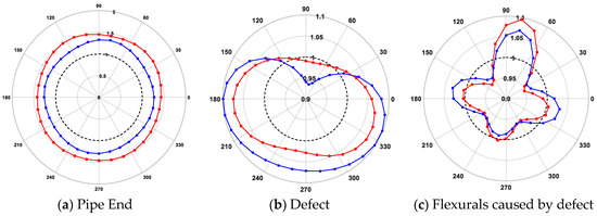
Figure 1.
Example of received FEM signals from the array from different sections of a pipe [31].
- The energy of waves received from axisymmetric features (e.g., pipe end) are overwhelmed by the T(0,1) with little variance caused by the existing coherent noise of flexural waves.
- Defect signals have a mixture of both flexural and torsional wave modes; nonetheless, if the cross-sectional area (CSA) of the defect is wide, the T(0,1) will have a greater effect than the flexurals. This is the main reason why adding all the transducers tends to increase the overall energy of T(0,1) while reducing the effect of flexurals.
- Noise regions are mostly consistent with flexurals with almost no axisymmetric wave being detected.
Furthermore, guided waves exhibit dispersive propagation. Dispersion causes the energy of a signal to spread out in space and time as it propagates [32]. Figure 2a shows an example of a dispersion curve calculated from an 8-inch schedule 40 steel pipe using RAPID software [33]. Wilcox et al. introduced a method to use dispersion curves in order to both simulate [34] and remove [32] the effect of dispersion. By applying the developed equation by Wilcox et al. and the shown dispersion curves in Figure 2a, a simulated propagation of F(4,2) wave mode is created and shown in Figure 2b where the black and red lines show the same wave mode after 1 m and 2 m of propagation, respectively. As can be seen, for a dispersive waveform the temporal resolution and the energy of wave packet is decreased. Therefore, in general inspection, non-dispersive regions of wave modes are excited to allow ease of inspection. In this research, T(0,1) is used as the excitation wave mode since it is non-dispersive across its whole frequency range [35].
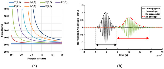
Figure 2.
(a) Example dispersion curve of T(0,1) wave mode in an 8-inch schedule 40 steel pipe. (b) The effect of dispersion on a simulated flexural wave, two propagation distances [31].
Three main signals are expected to be received in guided-wave tests which are shown in Figure 3. The first signal is the superposition of T(0,1) and flexurals where it is the true defect location. The second is the flexurals created due to wave mode conversion [36]; as these signals exhibit the same characteristics of excitation waveform, they can lead to the detection of false alarms. The third category is the non-coherent white noise, which is not correlated to the excitation sequence. This category is the main one which can be removed using generalized filtering techniques, as their characteristic is completely different to the excitation sequence.
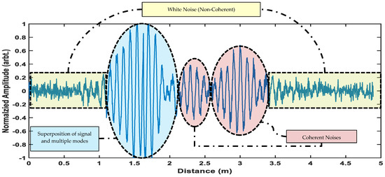
Figure 3.
Categories of the signals in the guided-wave inspection [31].
3. Methodology
As explained previously, guided waves are multimodal. To allow inspection of pipelines using guided waves, a single wave mode must be excited in only one direction to allow detection of the anomaly’s location. Excitation and detection of flexural waves are difficult and require complex processing algorithms due to their circumferential variation. Therefore, the practice in the general inspection is to excite an axisymmetric wave. For doing so, the toolset of guided-wave testing devices consists of arrays of linearly placed transducers (rings) across the circumference of the pipe. This leads to excitation of a quasi-axisymmetric wave where, in ideal scenarios, the corresponding flexurals of the excitation wave mode will cancel each other out [1,37,38]. If only one array is used, a bidirectional wave mode is generated since there is no directional control in the normal piezo-electric transducer. The most common method of achieving a unidirectional transmission is to use multiple arrays of transducers. By considering the dispersion curves of the generated wave mode and the placement spacing between the rings, waves can be manipulated in such a way to enforce the forward going propagation and suppress the backward leakage. Hence, the forward propagations of each ring are overlapped while the signals received from backward propagation direction are inversely overlapped [1,2,6,39].
On the reception side, signals from the backward direction will still be received due to (1) the impure/non-ideal excitation and (2) the forward propagation signals travel paths after the toolset. Once the device is in monitoring mode, no excitation takes place, meaning if an echo is received from the device, it will continue to travel past the test tool; if any anomalies exist in that direction, a new echo will be generated which will travel in the same way as the forward testing direction. At this point two scenarios will occur:
- In the first scenario, the signal from a feature in the backward test direction is detected by the rings. The energy of this signal can be reduced by using the same phase-delaying algorithm in the excitation sequence.
- The second scenario is when the same echo is past the tool. This signal will have the same characteristics as forward propagation and thus cannot be canceled. These are typically known as mirror signals.
The phase-delaying algorithm is once again applied in the general routine of reception to reduce the effect of signals generated from the first scenario. Afterward, the average of all transducer signals is generated, which will reduce the energy of flexural waves. The signal of the rings can also be strongly different which either suggests the existence of no defect or a small defect which is not generating a strong-enough signal to be detected. In the normal approach, as simple summation is used, this will lead to the generation of a residual signal which might be mistaken as a defect in the inspection. The flowchart for this general reception routine, which is the common practice of industry, is shown in Figure 4.
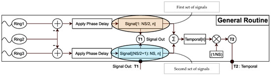
Figure 4.
Flowchart of general propagation routine currently used in guided-wave devices.
Adaptive Filtering
The main challenge in the inspection of guided waves is to decrease the energy of coherent noise in the test since non-coherent noise is generally removed by bandpass filtering and averaging. Dispersion characteristics of guided wave modes vary with regards to the structural features, frequency, and wave mode. However, the non-dispersive torsional mode is typically constant with an approximate speed of 3260 m/s. By shifting the rings to overlay the T(0,1) signals together, the wave modes which travel at different speeds will be less correlated with those that travel at constant speed. Furthermore, as shown in Figure 1, the flexural waves are highly variable in the space while the torsional mode has a higher correlation.
In this case, the existing torsional mode is highly correlated while the noise and flexural modes will be less correlated in time. Therefore, instead of the summation of the signals, adaptive filters can be utilized to enhance the signal resolution. The output signal of an finite impulse response (FIR) filter in time-domain can be achieved by the convolution operation using [10,40,41,42]:
where is the filter length, n is the iteration number, is the filter coefficients with the index of , and is the input signal. In the following equations, both and are vectors of size (represented by bold characters). The resultant error signal would be:
where represents the required reference (desired) signal; hence, in order to use this method, at least two signals are required. In adaptive filtering, the goal is to minimize the error signal by setting the filter weight. Therefore, in each iteration the filter weights should be updated:
where is the correction step applied to previous filter coefficients to update them for the next iteration; the key component of the adaptive filter is to define in a way that it decreases the mean square error over time. One of the robust methods is the normalized least mean square [20,41], which tries to minimize the least mean square error by setting the coefficients according to a variable step size. The formula is as follows:
where β is a normalized step size with 0 < β < 2, ϵ is some small positive number to bypass the problem when becomes too small. The noise in guided waves is highly variable due to the existence of time-varying multiple modes. To make sure the filter is not over-fitted to the characteristics of previous iterations, a leakage factor, , is added to reduce the effect of previous iterations [42]:
The flow chart of this algorithm is shown in Figure 5. In this setup, instead of adding the signals received from the rings of transducers, they are selected as the desired response and the input signal . Every other signal is updated based on the characteristics of each iteration and is the output of the filter. The selected reference and input signals are the two sets generated in the general propagation routine, as marked in Figure 4. Applying this phase delay and summation of arrays within each ring, two sets of signals are created where both have the following components:
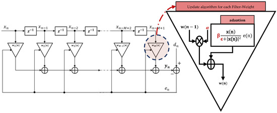
Figure 5.
Adaptive linear prediction algorithm for noise cancellation where the red marked parameters are fixed by the user.
- S(t) Signals of interest/anomalies: Highly correlated and in phase
- N(t) Flexural and other noise: That are not correlated to S(t). Furthermore, noise sources of two signals are correlated to each other.
This satisfies the need for a reference signal in using adaptive filtering. To cancel the backward leakage, this algorithm is done with the switching of the input and reference signals, where the final result is the summation of the two generated outputs of the adaptive filters.
4. Test Setup
The algorithm was initially developed on a synthesized data generated by FEM using ABAQUS software [30,43]. It was then validated in laboratory trials on real pipes using a Teletest Device [44].
4.1. Finite Element Model
The simulated pipe is based on the characteristics of an 8-inch schedule 40 steel pipe with a length of 6 m, outer diameter of 219.1 mm, thickness of 8.18 mm, Young’s Modulus of 210 GPa, density of 7850 and Poisson’s Ratio of 0.3. The excitation frequency in the test was 30 kHz. In order to capture the smallest wavelength in the operating frequency, at least 8 elements are required in the axial direction [45,46]. Therefore, the global seed size was set as 2.5 mm and the time increment was set as 3.11 × 10⁻⁷ s to provide a satisfactory accuracy in generation and reception of all the wave modes within the frequency band. The modeled test tool included 3 rings of 32 linearly spaced source points, located 1 m away from the back end of the pipe. Each source point of the rings is numbered clockwise starting from 90°. The schematic of this setup is illustrated in Figure 6.
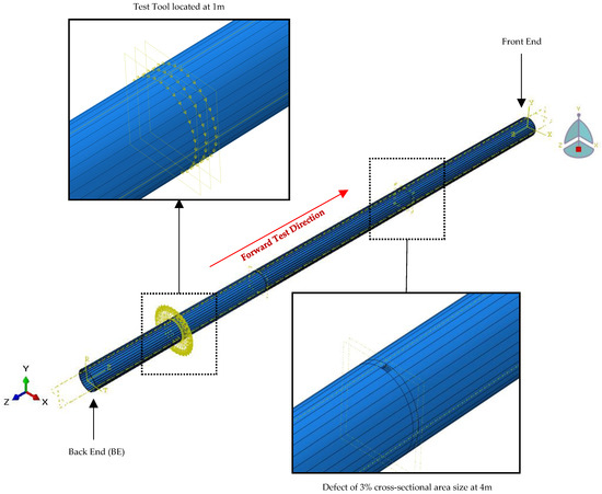
Figure 6.
Schematic of the FEM with test tool and defect located at 1 m and 4 m, respectively, from the back end [30].
This type of FEM synthesis of guided wave signals in pipes was developed in previous studies [37,46,47,48,49,50]. The generated models have also been validated by confirming the accuracy of the received signals from both the device [50], and 3D laser vibrometer [46,47]. Nonetheless, this type of FEM generally produces a limited amount of noise due to the perfect condition of the model. The main aim of this paper and the developed model is to investigate the performance of the algorithm in the presence of coherent noise. Therefore, in order to generate flexural noise in the test, different transfer functions were applied to the excitation sequence of each source point. Since the minimum satisfactory number of elements is used, the transfer functions will not affect the integrity of the model and all the existing wave modes in the test will be captured. Apart from these transfer functions, all other limits and parameters were in line with the verified models in the previous studies.
In 2013, Engineer [51] extracted the broadband frequency response of transducers with regards to various coupling forces using Teletest piezo-electric transducers. The reported frequency response was used as a reference and variability in terms of amplitude and phase was introduced to generate a variable transfer function for each transducer. An example is shown in Figure 7.
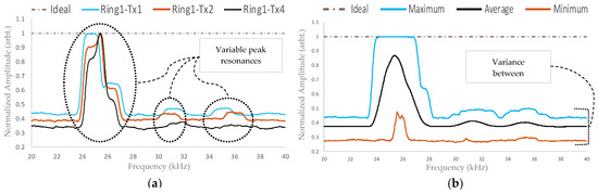
Figure 7.
Example of designed transfer functions wherein (a) three different source points are compared and (b) the maximum, average, and minimum amplitudes across all of the applied transfer functions used in an individual test are shown.
The transfer functions are multiplied by the ideal excitation’s frequency response, which is a 10 cycle 30 kHz Hann-windowed sine wave, and then inverted back into the time domain. The generated time-domain signals are used as input files for each of the source points. Additionally, the signals of the second array are phase delayed and inverted with regards to the 30 mm ring spacing cancellation algorithm [1,6]. The overall system works in the pulse-echo mode and the signals were received from the same ideal point sources. The signal generation, as well as the post-processing, were done using MATLAB-R2016a [52]. In order to increase the coherent noise of testing conditions, instead of receiving the signals from all source points, only source point numbers 1, 7, 14 and 26 of each ring have been used for reception (marked in red in Figure 8).
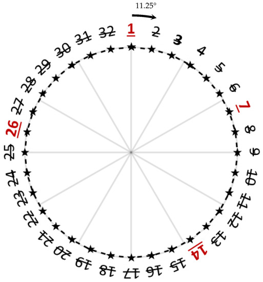
Figure 8.
The used reception points of each ring in the FEM.
The signal routes of the FEM test are shown in Figure 9. As can be seen, the first directly received signal from the forward test direction is the defect signal which is received at 3 m, followed by the front-end signal at 5 m. However, as the transfer function and reception points are not ideal, a backward leakage signal will exist, propagating in the forward direction. This leakage would be received at 1 m but due to the backward cancellation algorithm, it will not be observable. However, the reflection of this signal with the defect signal would be received from the forward direction, leading to a false alarm at 4 m. In these tests, since both signals at 3 and 4 m have the same characteristics, they are both considered defect signals even though the second signal is a false detection.
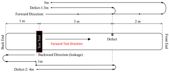
Figure 9.
Torsional mode reception route in the FEM test cases.
4.2. Experimental Trials
In the laboratory trials, a Teletest MK4 device [44] was used in order to inspect an 8-inch schedule 40 steel pipe with a length of 6 m. The test tool included a collar of 3 ring transducers with 30 mm ring spacing, located 1.5 m away from the back end of the pipe. Each ring included 24 linearly spaced thickness-shear (d15) piezoelectric transducers. The system provided both excitation and reception of signals in pulse-echo mode with the operating frequency of 20 to 100 kHz. The device can capture the transducers’ signals with a sampling frequency of 1 MHz. On the reception side, an internal bandpass filter was applied to filter any frequencies outside the main bandwidth of the excitation bandwidth. The device outputs the time-domain signal received from each ring, as well as the processed signal with the general propagation routine. In this paper, the signals from the rings are extracted in order to apply the algorithm.
The defects in these trials are located 4.5 m from back end of the pipe (3 m away from the test tool). The defects were introduced by removing the pipe’s surface material with a saw. The defect sizes were varying from 3% to 8% CSA with steps of 1% CSA (total of 6 defect sizes). The signal routes of the laboratory trials are shown in Figure 10. As opposed to the FEM test setup, the Defect-2 signal, which was generated by reflection of backward leakage signal from the defect, is now overlapped with the front-end signal and is no longer detectable.
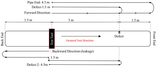
Figure 10.
Torsional mode reception route for laboratory trials.
5. Results
In order to better understand this process, an example test case is initially shown where each stage of the algorithm is explained thoroughly. Then the experimental results are demonstrated in the second part of this section where the SNRs are calculated with regards to defects with different CSA sizes and excitation frequencies. In both cases the SNRs are calculated based on the following formula:
where Signal is considered the window where the energy of the signal is received (between 3.0 m and 3.5 m depending on the frequency) and everything else is considered noise. In both tests, excitation sequences are 10-cycle Hann-windowed sine waves.
5.1. Example Test Case
This technique is initially developed and validated on synthesized data generated by FEM. The used excitation sequence for generating this data set is 30 kHz and variable transfer functions were used for each of the source points. Figure 11 shows the two sets of signals achieved after applying the phase delays of general propagation routine (blue and red). Four regions are of main interest in this figure, which are (a) backward leakage, (b) flexural noise, (c) Defect-1 and (d) Defect-2. Since both Defect-1 and Defect-2 signals are received from the forward testing direction, they have similar characteristics and thus both should be enhanced by this algorithm. As can be seen, noise region (b) is significantly less correlated than the defect signals (c and d). Furthermore, although the amplitudes of two sets of signals received in the defect regions are not the same, their phases and polarity are in perfect correlation. Therefore, while in the propagation routine their characteristic might be similar but, in this space, the defect and flexural signals are distinguishable.
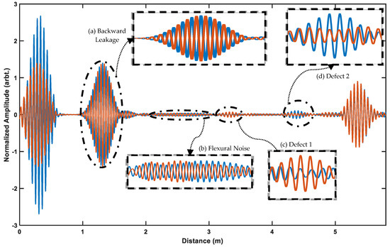
Figure 11.
FEM signals (30 kHz) where two defect regions and the flexural noises are marked where blue and red lines show the first and second sets of the signals respectively.
5.2. Cancellation of Backward Leakage
Figure 11a shows the two sets of signals received from the backward testing direction. As can be seen, these signals are inversely overlapped with little differences in amplitude. This is due to the general propagation routine where the received signals from rings are delayed and inverted depending on the ring spacing.
After applying the filtering, the phase of the outcome does not change, therefore by switching the inputs to the adaptive filter, two sets of results will be generated in which the signals from the forward direction are overlapped and the ones from the backward direction are inversely overlapped. This is illustrated in Figure 12, where blue and red signals show the two sets of results achieved from adaptive filtering by switching the inputs. This operation not only enhances the defect signals received from the forward direction (Figure 12c) but it also decreases both the backward cancellation (Figure 12a) and flexural noise regions (Figure 12b) significantly.
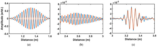
Figure 12.
Two sets of results after swapping the inputs to adaptive filter where (a) shows the signals received from the backward direction, (b) shows the flexural noise, and (c) shows the defect signal.
5.3. Adaption of Filter Weights
The used filter order in the tests is five, which means only five past samples are required to process the results (Appendix A). Since the number of available samples is limited, observation of the filter’s frequency response is not possible. Therefore, in Figure 13b–f, the changes of the first filter value are shown while Figure 13a shows their corresponding results in the time-domain. The red signals illustrate the results of the leaky-NLMS while the black dotted lines represent the normal NLMS algorithms. While normal NLMS depends more on past values and is not fast to adapt to the current iteration, leaky NLMS makes this adaption faster by reducing the filter weights’ dependence on their past values. After each adaption to a big sequence such as backward leakage or defect, the magnitude of the filter weight tends to move toward zero; in other words, the weights forget the characteristics of past iterations significantly faster, which allows them a quicker adaption to the characteristic of the current iteration. Furthermore, as illustrated by blue dotted signals, in the region of defects, a high peak is generated in the magnitude of each filter order set by the leaky-NLMS method. Although other techniques and updated algorithms exist, this fast adaption algorithm, where the filter can forget the characteristics of the previous wave, is the main reason why leaky-NLMS is more effective in the guided-wave inspection of pipelines.
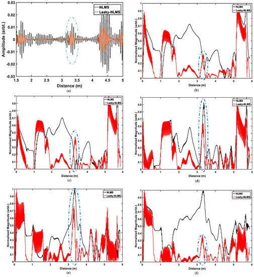
Figure 13.
Comparison of the result achieved from NLMS (black) vs leaky LMS (orange) where (a) shows the time-domain results and (b–f) show the normalized magnitudes of filter order 1 to 5, respectively.
5.4. Results Comparison
The performance of the algorithm was assessed in experimental trials by detecting defects of CSA sizes between (and including) 3% and 8%. It is expected that the algorithm would be more effective at lower frequencies since they are more dispersive; furthermore, the excitation power of lower frequencies is higher than those of higher frequencies, both due to the duration of the signals as well as the systems transfer function. Therefore, frequencies between 30 to 50 kHz with a step of 2 kHz were tested. The SNR achieved from the general propagation routine is demonstrated in Appendix B. The peak SNR is always achieved using 40 kHz excitation frequency where the SNR decreases by moving toward either side of that frequency. Furthermore, the SNRs achieved from each frequency are reduced almost linearly when the defect size is decreased; thus, the noise energy is almost constant while the defect energy is decreasing.
5.4.1. Parameter Selection
The results were generated from two sets of parameters (given in Appendix C Table A3):
- Model Parameters: The optimum parameters are achieved by using a brute force search algorithm to find the parameters which give the maximum SNR in the FEM test. The main goal of this test was to assess the response of the algorithm by fixing the parameters to an optimum solution created by the FEM.
- Experimental Parameters: The brute force search algorithm was performed on the 4% CSA sample to find parameters that result in most enhancements of SNR for each frequency. The goal was to find the best testing frequency where the least variations in the enhancements are observed and assess whether fixed parameters can enhance the SNR of defects with lower CSA size (3% test case).
5.4.2. Model-Parameters
The results achieved from model parameters are shown in Figure 14 where (a) shows the achieved SNR values and (b) shows the amount of enhancement. The following conclusions can be extracted from these tests:
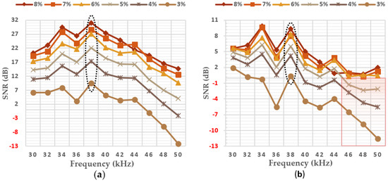
Figure 14.
Results achieved using fixed model parameters for all frequencies where (a) shows the achieved SNR and (b) shows the amount of improvement in comparison to the general propagation routine.
- In defects above 5% CSA, the algorithm enhances the results using all frequencies. For defects with CSA size of lower than 4%, the algorithm can enhance the SNR of most frequencies except for 30, 32, 34, and 38 kHz.
- Except from the case of 3% CSA error, both maximum SNR and maximum enhancements are achieved using 34 and 38 kHz in the tests. In the 3% CSA test, the maximum enhancement is for 30 kHz; nonetheless, the final SNRs of 34 and 38 kHz are greater.
- The variations in the case of 30 kHz are less in comparison to all other cases, as shown in Figure 14b.
5.4.3. Experimental Parameters
The results of experimental parameters are illustrated in Figure 15. The following conclusions can be drawn from these tests:
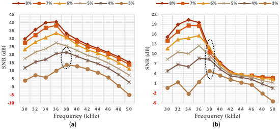
Figure 15.
Results achieved using experimental parameters, which are variable for each frequency, where (a) shows the achieved SNR and (b) shows the amount of improvement compared to the general propagation routine.
- For defects with higher CSA error size (above 5%), lower frequencies tend to achieve higher SNR after processing where the defect signal was enhanced by at least a factor of 2. The greatest enhancement is achieved from 34 kHz and the maximum SNR is achieved from 36 kHz for these signals.
- Although higher frequencies will result in lower SNR, their enhancements are approximately the same for different sizes of the defect. Nonetheless, their final SNR is almost always lower than all other frequencies, especially in the cases of frequencies above 46 kHz.
- For 3% and 4% CSA defects, the greatest enhancement and gain are achieved using the 38 kHz frequency. Furthermore, as can be seen in Figure 15b, this frequency is affected less with regards to the CSA loss of the defect.
5.4.4. Discussion
Figure 16 shows the difference of enhancements between the results of model parameters and experimental parameters. These results show that although temporal SNR of the signals is important, the spatial characteristic of the noise also plays an important role in the amount of enhancement. As an example, while 40 kHz has the highest SNR from the general routine, it does not perform as well as 38 kHz for the algorithm. In most cases of lower CSA defects, the SNR improvements are achieved not by enhancing the axisymmetric signal strength, but by removing the flexural noise. Except for excitation frequencies of 30, 34, and 40 kHz in the 3% CSA defect, all other cases were enhanced when the experimental parameters were used.
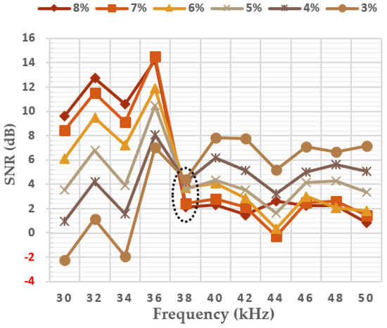
Figure 16.
Amount of improvement achieved by experimental parameters as opposed to model parameters.
Since signals with SNRs higher than 30 dB are more easily detected, it is better to use a frequency which provides a stable enhancement for both low and higher CSA sizes rather than setting parameters which can greatly increase the higher CSA defects while decreasing the SNR of smaller defects. An excitation frequency of 38 kHz provides approximately the same enhancement using both model parameters and experimental parameters, which shows that this frequency is less affected by the parameters in comparison to the others. Furthermore, it can also be seen from the results of model parameters that 38 kHz always achieves the maximum gain even though the parameters are optimized for 30 kHz excitation frequency in the model.
All frequencies above 40 kHz fail to provide any improvements for defects with CSA sizes smaller than 4% using model parameters. Nonetheless, even the enhancements achieved with experimental parameters in those frequencies are much less than all other frequencies, which suggests that this algorithm tends to perform better at lower frequencies. This is expected since flexurals with lower frequencies are highly dispersive, which adds to the spatial noise of the tests.
It should be born in mind that, even though in some frequencies the mathematically calculated SNR might be less than the one achieved from the general propagation routine, the high-order flexurals are always canceled, which leads to easier interpretation of results by the inspectors. Figure 17 shows the results of the 30 kHz excitation sequence for defects with different CSAs. As can be seen, highly variable noises in the region between 2.5 and 3 m are canceled but those caused by low order flexurals at 2 to 2.5 m are enhanced. While in defects with higher CSA sizes most improvement is achieved due to the amplification of the defect signal, in lower CSA defects (especially in the case of 3% CSA), the noise cancellation is the main reason for enhancement. The enhancement of these low order flexurals is the main reason why the algorithm fails to improve the SNR in some of the testing frequencies. With regards to the dispersion curves (Figure 2a), low order flexurals become non-dispersive on frequencies above 30 kHz with their speed moving toward that of T(0,1), 3260 m/s. Since the phase delays are applied with respect to T(0,1) wave speed, if the flexural waves have the same speed they will be overlapped in the input and desired responses. This is the main reason why such signals might not be canceled and, in fact, in some scenarios, they might even be amplified. Furthermore, considering the 34 kHz filtered signal shown in Figure 18b, the noise envelope is clearly dispersed (2–2.5 m). Figure 19 also shows the results achieved from 38 kHz excitation frequency. In these figures, the input and reference signals for the noise and defect regions are shown as blue and red. The following conclusions can be extracted by observing the difference between a defect and noise signals:
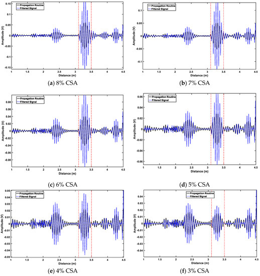
Figure 17.
Example of filtered signals using 30 kHz excitation and model parameters where defect size is varying.
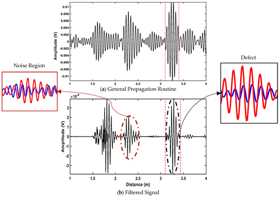
Figure 18.
The result of (a) general propagation routine vs (b) filtered signal with their corresponding inputs (blue and red lines) of noise (left side) and defect (right side) with the excitation frequency of 34 kHz gathered from an experimental pipe with defect size of 3% CSA.
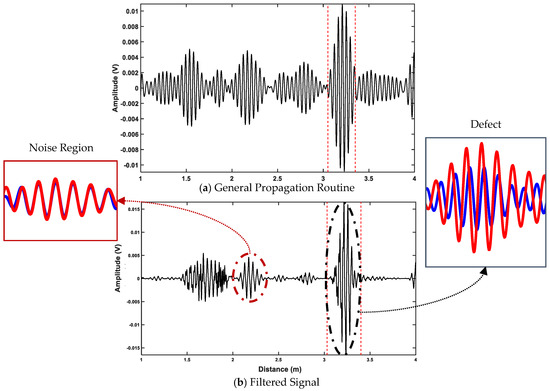
Figure 19.
The result of (a) general propagation routine vs (b) filtered signal with their corresponding inputs (blue and red lines) of noise (left side) and defect (right side) with the excitation frequency of 38 kHz gathered from an experimental pipe with defect size of 3% CSA.
- If any low order flexurals or noise are overlapping in the input and reference signals, they will not be removed and might be amplified.
- Although some flexural signals will remain in the resultant signal, there is an option of further post-processing to enhance the SNR. Such is the case of the noise region located at 2–2.5 m in case Figure 18, where it is clearly dispersed at the end of its window, and the case of 1.5–2 m in Figure 19, which results from backward leakage. Therefore, by considering other characteristics in the signal, the results can be post-processed to distinguish different modes and further increase the SNR of the test.
6. Conclusions
In this paper, an adaptive filtering approach is utilized to enhance the SNR of the torsional waves generated from defects in guided wave inspection of pipelines. For doing so, as opposed to using a general propagation routine of guided-wave testing devices, the two sets of signals received from the test tool were used as inputs to the adaptive filter, which resulted in a single output in the time domain. Inherently, in these two sets of signals, the torsional waves are overlapping while the flexurals are varying; this was the basis on which the adaptive filter was able to enhance the SNR of torsional waves. Since flexural waves are variable both in space and time, the used updated algorithm for filter weights was leaky NLMS, which allowed faster adaption to the highly variable flexural noise and enabled a faster reset of the filter weights.
The algorithm was initially developed and validated using the synthesized signal generated from an FEM test case. Afterward, laboratory trail validation took place with two sets of filter parameters: model parameters, where the parameters were set to find the highest SNR for the FEM test case with excitation frequency of 30 kHz; and experimental parameters, where the optimum parameters for each frequency were generated with regards to the real pipe data with 4% CSA defect. In most test cases, all the frequencies resulted in enhancement of the SNR. Nonetheless, the optimum testing frequency was found to be 38 kHz since it achieved both the maximum and greatest enhancement of SNR in tests with defects. Also, this excitation frequency was less affected by the change of parameter as limited enhancement was observed between the results achieved by using model parameters and experimental parameters.
Comparing the results from model parameters and experimental parameters, it is evident that setting the parameters with regards to each individual frequency enhances the achieved SNR. Nonetheless, optimum selection of parameters is a trade-off between the maximum achieved gain and the stable enhancement of the SNR of smaller defects. This was assessed using experimental parameters; when the optimum parameters for 4% CSA defect were used for the case of 3% defect, not all frequencies could improve the SNR. The model parameters test proved that the parameters can be chosen using an FEM model, but it will not result in the maximum gain.
The amount of SNR achieved in each test case depends not only on the enhancements of the torsional wave but also the cancellation of the flexural waves. It must be borne in mind that since the physical arrangement of the rings is fixed, in some cases, especially for lower order flexural waves that have closer wave speeds to torsional waves, noise will not be canceled. However, the higher order flexural noise will be canceled in all the tests and the achieved results can be further processed for torsional wave mode detection.
Author Contributions
Conceptualization, H.N.M. and A.K.N.; methodology, H.N.M. and A.K.N.; software, H.N.M.; validation, H.N.M.; formal analysis, H.N.M.; investigation, H.N.M.; resources, H.N.M.; data curation, H.N.M.; writing—original draft preparation, H.N.M.; writing, reviewing and editing, H.N.M., K.Y., and A.K.N.; visualization, H.N.M. and A.K.N.; supervision, K.Y. and A.K.N.
Funding
This publication was made possible by the sponsorship and support of Brunel University London and National Structural Integrity Research Centre (NSIRC).
Conflicts of Interest
The authors declare no conflicts of interest.
Appendix A
The filter order was selected based on the FEM data. A brute force search was applied to maximize the SNR of Defect-1, calculated by Equation (6). Therefore, the best case of each weight is considered. The generated results are shown in Table A1. The SNR of the unfiltered signal is 5.3 dB. Therefore, this signal is more difficult to detect as it is almost buried in the noise level. As can be seen, by increasing the filter order, the SNR is reduced. When the size of filter order grows above 8, the SNRs of filtered and unfiltered signals are approximately the same. This is because by growing the number of samples, the differences between a torsional and flexural wave become limited as they are in the same frequency band. However, in smaller steps, the changes in flexural waves are more time-varying. Therefore, from these results, 8 can be the considered as the safest number for filter order where no change will be applied to the signal and 2 can be considered as the best filter order for maximizing the SNR.
On the other hand, the best filter order can be dependent on other factors, such as frequency and the existing flexurals of the iteration. Since the main aim of this paper is to test the workability of the adaption algorithm to the guided-wave scenario, the filter order is fixed to 5. This number is a compromise between the safest choice, 8, and the best achieved results, 2, based on FEM with 30 kHz excitation sequence. Furthermore, a filter order of 5 can be considered as a good compromise, as a drop of only 1 dB is observed from the maximum achieved SNR, which is 8.31 dB.

Table A1.
Maximum SNR achieved for each filter order on FEM test signal with 30 kHz signal.
Table A1.
Maximum SNR achieved for each filter order on FEM test signal with 30 kHz signal.
| Filter Order (#) | 2 | 3 | 4 | 5 | 6 | 7 | 8 | 9 | 10 |
|---|---|---|---|---|---|---|---|---|---|
| Maximum SNR (dB) | 8.31 | 8.27 | 7.76 | 7.32 | 6.78 | 6.07 | 5.33 | 5.07 | 5.02 |
Appendix B
The SNR of the defect signal achieved from the general propagation routine of the device is demonstrated in Table A2 and Figure A1.
Table A2.
SNR achieved from the general propagation routine (in dB).
Table A2.
SNR achieved from the general propagation routine (in dB).
| CSA | Frequency (kHz) | ||||||||||
|---|---|---|---|---|---|---|---|---|---|---|---|
| (%) | 30 | 32 | 34 | 36 | 38 | 40 | 42 | 44 | 46 | 48 | 50 |
| 8 | 14.68 | 16.81 | 19.64 | 21.04 | 21.73 | 22.28 | 21.84 | 20.47 | 18.33 | 15.70 | 12.63 |
| 7 | 13.55 | 15.50 | 18.19 | 19.69 | 20.64 | 21.39 | 20.97 | 19.48 | 17.20 | 14.53 | 11.38 |
| 6 | 11.70 | 13.57 | 15.89 | 17.88 | 18.78 | 19.33 | 18.75 | 17.27 | 15.06 | 12.40 | 9.24 |
| 5 | 9.29 | 11.09 | 13.71 | 15.00 | 16.05 | 16.74 | 16.05 | 14.40 | 12.07 | 9.38 | 6.17 |
| 4 | 7.13 | 8.84 | 11.12 | 12.15 | 13.13 | 13.76 | 13.23 | 11.73 | 9.50 | 6.84 | 3.50 |
| 3 | 4.29 | 5.97 | 8.15 | 8.62 | 9.08 | 9.51 | 9.00 | 7.60 | 5.43 | 2.82 | −0.51 |

Figure A1.
SNR of tests using general propagation routine.
Appendix C
Table A3 shows the parameters used in each test with regards to the frequency.
Table A3.
Used parameters in the tests.
Table A3.
Used parameters in the tests.
| Frequency (kHz) | Step Size | Leakage | Compensation |
|---|---|---|---|
| 30 (Model) | 0.01 | 0.96 | 0.01 |
| 30 | 0.01 | 0.61 | 0.21 |
| 32 | 0.01 | 0.46 | 0.21 |
| 34 | 0.01 | 0.46 | 0.26 |
| 36 | 0.01 | 0.56 | 0.06 |
| 38 | 0.16 | 0.81 | 0.01 |
| 40 | 0.86 | 0.76 | 0.01 |
| 42 | 1.41 | 0.91 | 0.01 |
| 44 | 1.21 | 0.96 | 0.01 |
| 46 | 1.46 | 0.96 | 0.01 |
| 48 | 1.46 | 0.96 | 0.01 |
| 50 | 1.46 | 0.96 | 0.01 |
References
- Lowe, M.J.S.; Alleyne, D.N.; Cawley, P. Defect detection in pipes using guided waves. Ultrasonics 1998, 36, 147–154. [Google Scholar] [CrossRef]
- Pavlakovic, B. Signal Processing Arrangment. US Patent 2006/0203086 A1, 14 Septenber 2006. [Google Scholar]
- ASTM Standard E2775-16. Standard Practice for Guided Wave Testing of above Ground steel Pipeword Using Piezoelectric Effect Transducer; ASTM: West Conshohocken, PA, USA, 2017. [Google Scholar]
- Yücel, M.K.; Fateri, S.; Legg, M.; Wilkinson, A.; Kappatos, V.; Selcuk, C.; Gan, T.H. Coded Waveform Excitation for High-Resolution Ultrasonic Guided Wave Response. IEEE Trans. Ind. Inform. 2016, 12, 257–266. [Google Scholar] [CrossRef]
- Fateri, S.; Boulgouris, N.V.; Wilkinson, A.; Balachandran, W.; Gan, T.H. Frequency-sweep examination for wave mode identification in multimodal ultrasonic guided wave signal. IEEE Trans. Ultrason. Ferroelectr. Freq. Control 2014, 61, 1515–1524. [Google Scholar] [CrossRef]
- Thornicroft, K. Ultrasonic Guided Wave Testing of Pipelines Using a Broadband Excitation. Ph.D Thesis, Brunel University London, London, UK, 2015. [Google Scholar]
- Malo, S.; Fateri, S.; Livadas, M.; Mares, C.; Gan, T. Wave Mode Discrimination of Coded Ultrasonic Guided Waves using Two-Dimensional Compressed Pulse Analysis. IEEE Trans. Ultrason. Ferroelectr. Freq. Control 2017, 64, 1092–1101. [Google Scholar] [CrossRef] [PubMed]
- Pedram, S.K.; Fateri, S.; Gan, L.; Haig, A.; Thornicroft, K. Split-spectrum processing technique for SNR enhancement of ultrasonic guided wave. Ultrasonics 2018, 83, 48–59. [Google Scholar] [CrossRef]
- Mallet, R. Signal Processing for Non-Destructive Testing. Ph.D Thesis, Brunel Unviersity, London, UK, 2007. [Google Scholar]
- Hayes, M.H. Statistical Digital Signal Processing and Modeling; John Wiley & Sons, Inc.: New York, NY, USA, 1997. [Google Scholar]
- Bellanger, M.G. Adaptive Digital Filters, Revised and Expanded, 2nd ed.; Marcel Dekker, Inc.: New York, NY, USA, 2001. [Google Scholar]
- Widrow, B.; Glover, J.R.; McCool, J.M.; Kaunitz, J.; Williams, C.S.; Hearn, R.H.; Zeidler, J.R.; Dong, J.E.; Goodlin, R.C. Adaptive Noise Cancelling: Principles and Applications. Proc. IEEE 1975, 63, 1692–1716. [Google Scholar] [CrossRef]
- Rajesh, P.; Umamaheswari, K.; Kumar, V.N. A Novel Approach of Fetal ECG Extraction Using Adaptive Filtering. Int. J. Inf. Sci. Intell. Syst. 2014, 3, 55–70. [Google Scholar]
- Hernandez, W. Improving the response of a wheel speed sensor using an adaptive line enhancer. Measurement 2003, 33, 229–240. [Google Scholar] [CrossRef]
- Ramli, R.M.; Noor, A.O.A.; Samad, S.A. A Review of Adaptive Line Enhancers for Noise Cancellation. Aust. J. Basic Appl. Sci. 2012, 6, 337–352. [Google Scholar]
- Murano, K.; Unagami, S.; Amano, F. Echo Cancellation and Applications. IEEE Commun. Mag. 1990, 28, 49–55. [Google Scholar] [CrossRef]
- Messerrschmi, D. Echo Cancellation in Speech and Data Transmission. IEEE J. Sel. Areas Commun. 1984, 2, 283–297. [Google Scholar] [CrossRef]
- Bürger, W. Space-Time Adaptive Processing: Fundamentals. Adv. Radar Signal Data Process. 2006, 6, 1–14. [Google Scholar]
- Schwark, C.; Cristallini, D. Advanced multipath clutter cancellation in OFDM-based passive radar systems. In Proceedings of the 2016 IEEE Radar Conference (RadarConf 2016), Philadelphia, PA, USA, 2–6 May 2016. [Google Scholar]
- Zhu, Y.; Weight, J.P. Ultrasonic nondestructive evaluation of highly scattering materials using adaptive filtering and detection. IEEE Trans. Ultrason. Ferroelectr. Freq. Control. 1994, 41, 26–33. [Google Scholar]
- Monroe, D.; Ahn, I.S.; Lu, Y. Adaptive filtering and target detection for ultrasonic backscattered signal. In Proceedings of the 2010 IEEE International Conference on Electro/Information Technology, Normal, IL, USA, 20–22 May 2010. [Google Scholar]
- Haykin, S. Adaptive Filter Theory, 5th ed.; Pearson: Harlow, UK, 2014. [Google Scholar]
- Cioffi, J. Limited-Precision Effects in Adaptive Filtering [invited paper, special issue on adaptive filtering. IEEE Trans. Circuits Syst. 1987, 34, 821–833. [Google Scholar] [CrossRef]
- Sayed, A.H.; Al-Naffouri, T.Y. Mean-square analysis of normalized leaky adaptive filters. In Proceedings of the 2001 IEEE International Conference on Acoustics, Speech, and Signal Processing (Cat. No.01CH37221), Salt Lake City, UT, USA, 7–11 May 2001; Volume 6, pp. 3873–3876. [Google Scholar]
- Bismor, D.; Pawelczyk, M. Stability Conditions for the Leaky LMS Algorithm Based on Control Theory Analysis. Arch. Acoust. 2016, 41, 731–739. [Google Scholar] [CrossRef]
- Lowe, M.J.S.; Cawley, P. Long Range Guided Wave Inspection Usage—Current Commercial Capabilities and Research Directions; Imperial College London: London, UK, 2006; Available online: http://www3.imperial.ac.uk/pls/portallive/docs/1/55745699.PDF (accessed on 20 November 2018).
- Meitzler, A.H. Mode Coupling Occurring in the Propagation of Elastic Pulses in Wires. J. Acoust. Soc. Am. 1961, 33, 435–445. [Google Scholar] [CrossRef]
- Catton, P. Long Range Ultrasonic Guided Waves for Pipelines Inspection; Brunel University: London, UK, 2009. [Google Scholar]
- Nurmalia. Mode Conversion of torsional Guided Waves for Pipe Inspection: An electromagnetic Acoustic Transducer Technique; Osaka University: Osaka Prefecture, Japan, 2013. [Google Scholar]
- Nakhli Mahal, N.; Mudge, P.; Nandi, A.K. Comparison of coded excitations in the presence of variable transducer transfer functions in ultrasonic guided wave testing of pipelines. In Proceedings of the 9th European Workshop on Structural Health Monitoring, Manchester, UK, 10–13 July 2018. [Google Scholar]
- Nakhli Mahal, N.; Muidge, P.; Nandi, A.K. Noise removal using adaptive filtering for ultrasonic guided wave testing of pipelines. In Proceedings of the 57th Annual British Conference on Non-Destructive Testing, Nottingham, UK, 10–12 September 2018; pp. 1–9. [Google Scholar]
- Wilcox, P.D. A rapid signal processing technique to remove the effect of dispersion from guided wave signals. IEEE Trans. Ultrason. Ferroelectr. Freq. Control 2003, 50, 419–427. [Google Scholar] [CrossRef]
- Sanderson, R. A closed form solution method for rapid calculation of guided wave dispersion curves for pipes. Wave Motion 2015, 53, 40–50. [Google Scholar] [CrossRef]
- Wilcox, P.; Lowe, M.; Cawley, P. The effect of dispersion on long-range inspection using ultrasonic guided waves. NDT E Int. 2001, 34, 1–9. [Google Scholar] [CrossRef]
- Guan, R.; Lu, Y.; Duan, W.; Wang, X. Guided waves for damage identification in pipeline structures: A review. Struct. Control Health Monit. 2017, 24, e2007. [Google Scholar] [CrossRef]
- Lowe, M.J.S.; Alleyne, D.N.; Cawley, P. The Mode Conversion of a Guided Wave by a Part-Circumferential Notch in a Pipe. J. Appl. Mech. 1998, 65, 649–656. [Google Scholar] [CrossRef]
- Miao, H.; Huan, Q.; Wang, Q.; Li, F. Excitation and reception of single torsional wave T(0,1) mode in pipes using face-shear d24 piezoelectric ring array. Smart Mater. Struct. 2017, 26, 025021. [Google Scholar] [CrossRef]
- Rose, J.L. Ultrasonic Guided Waves in Solid Media; Cambridge University Press: New York, NY, USA, 2014. [Google Scholar]
- Alleyne, D.N.; Pavlakovic, B.; Lowe, M.J.S.; Cawley, P. Rapid, Long Range Inspection of Chemical Plant Pipework Using Guided Waves. Key Eng. Mater. 2004, 270–273, 434–441. [Google Scholar] [CrossRef]
- Douglas, S.C. Performance Comparison of Two Implementations of the Leaky LMS Adaptive Filter. IEEE Trans. Signal Process. 1997, 45, 2125–2129. [Google Scholar] [CrossRef]
- Cartes, D.A.; Ray, L.R.; Collier, R.D. Experimental evaluation of leaky least-mean-square algorithms for active noise reduction in communication headsets. J. Acoust. Soc. Am. 2002, 111, 1758–1771. [Google Scholar] [CrossRef] [PubMed]
- Kuo, S.M.; Lee, B.H.; Tian, W. Real-Time Digital Signal Processing: Implementations and Applications; John Wiley & Sons: Chichester, UK, 2006. [Google Scholar]
- Ssanalysis. Abaqus/Explicit. Available online: http://www.ssanalysis.co.uk/ (accessed on 20 Nov 2018).
- Teletestndt. Long Range Guided Wave Testing with Teletest Focus+. 2018. Available online: https://www.teletestndt.com/ (accessed on 08 January 2019).
- Alleyne, D.N.; Lowe, M.J.S.; Cawley, P. The Reflection of Guided Waves from Circumferential Notches in Pipes. J. Appl. Mech. 1998, 65, 635–641. [Google Scholar] [CrossRef]
- Lowe, P.S.; Sanderson, R.M.; Boulgouris, N.V.; Haig, A.G. Inspection of Cylindrical Structures Using the First Longitudinal Guided Wave Mode in Isolation for Higher Flaw Sensitivity. IEEE Sens. J. 2016, 16, 706–714. [Google Scholar] [CrossRef]
- Niu, X.; Duan, W.; Chen, H.; Marques, H.R. Excitation and propagation of torsional T (0, 1) mode for guided wave testing of pipeline integrity Excitation and propagation of torsional T (0, 1) mode for guided wave testing of pipeline integrity. Measurement 2018, 131, 341–348. [Google Scholar] [CrossRef]
- Duan, W.; Niu, X.; Gan, T.; Kanfound, J.; Chen, H.-P. A Numerical Study on the Excitation of Guided Waves. Metals 2017, 7, 552. [Google Scholar] [CrossRef]
- Fateri, S.; Lowe, P.S.; Engineer, B.; Boulgouris, N.V. Investigation of ultrasonic guided waves interacting with piezoelectric transducers. IEEE Sens. J. 2015, 15, 4319–4328. [Google Scholar] [CrossRef]
- Alleyne, D.N.; Cawley, P. The excitation of Lamb waves in pipes using dry-coupled piezoelectric transducers. J. Nondestruct. Eval. 1996, 15, 11–20. [Google Scholar] [CrossRef]
- Engineer, B.A. The Mechanical and Resonant Behaviour of a Dry Coupled Thickness-Shear PZT Transducer Used for Guided Wave Testing in Pipe Line. Ph.D Thesis, Brunel University, London, UK, 2013. [Google Scholar]
- Mathworks. Matlab. Available online: https://uk.mathworks.com/products/matlab.html (accessed on 18 April 2018).
© 2019 by the authors. Licensee MDPI, Basel, Switzerland. This article is an open access article distributed under the terms and conditions of the Creative Commons Attribution (CC BY) license (http://creativecommons.org/licenses/by/4.0/).