A Collaborative Human-Robot Framework for Visual Topological Mapping of Coral Reefs

Featured Application

The proposed method is applied to the collaborative topological mapping of coral reefs using visual information captured by humans and/or robots with the aim of creating richer representations of the environment.

Abstract

One of the most important tasks when creating a map of visual information obtained from different agents is finding common locations between the sets of images that enable them to be fused into a single representation. Typical approaches focus on images obtained from the same agent. However, in this paper, we focus on recognizing the same places in images captured by different agents to create a topological map of coral reefs. The main components of the proposed method are the voting scheme to find a sparse similarity matrix between different frames and an effective method to match sequences of images exploiting the sparsity of the resulting similarity matrix. We have applied our method to sequences of images obtained from coral reef explorations performed by different agents. The presented method shows a good performance compared to other well-established methods such as FABMAP. This demonstrates its ability to find common locations from visual information gathered from different sources, which eases the collaboration between humans and robots to map the environment.

1. Introduction

Although robots are widely used in underwater environments to create maps (topological maps or seafloor mosaics), these are typically created by a single robotic agent without interaction or support from other agents. Adding help from other agents can benefit the created map by enriching with more information from cameras with better resolution or even with information from other points of view. In addition to the use of other robotic agents, it can be helpful to include information captured by humans into the mapping process. A diver could provide images from parts of the coral reef that are of interest to other researchers. For example, while a robot can be programmed to follow a zig-zag trajectory above a coral reef, a human can navigate the same environment closer to certain species of coral, thereby providing detailed images from the areas of interest. However, creating a map of information from more than one agent is not trivial, specifically because it is necessary to recognize the same places in images taken with different cameras, under different environmental conditions, and with different points of view. Moreover, the information captured by a diver can be more challenging to handle with regard to point of view variations because it is more difficult for human explorers in these environments to maintain a constant orientation and distance with respect to the seafloor compared to robotic agents. Therefore, to recognize places in different images (loop closure detection), whether they are captured by the same agent or not, one of the most relevant challenges to tackle is generating a robust image description that allows the identification of two images taken from the same place despite changes in appearance and point of view. It also should be distinctive enough to discard two similar images from different places.

With respect to the image description, there are two main approaches: using a global descriptor for the whole image (e.g., Pyramid Histogram of Oriented Gradients [1]) or describing an image with respect to the contained local features (e.g., Speed-Up Robust Features [2]). However, combinations of both approaches can also be applied. One of the most known methods for visual place recognition is FAB-MAP [3], where local features are used to generate a Bag of Visual Words (BoVW) [4] to describe images with respect to the frequency of occurrence of features contained in a codebook or dictionary. This method uses a Chow-Liu tree to approximate the dependency between the occurrence of the detected visual features. They have obtained very good results for outdoor environments despite the existence of perceptual aliasing (i.e., images that are perceptually similar but from different scenes). A dictionary or codebook for this kind of method is a collection of representative visual features that can be found in the environment of interest and it is typically built by clustering similar local features extracted from a sample of images of the environment. The use of a dictionary helps to improve the efficiency of the method, as an image can be described only in terms of the presence of the features contained in the dictionary.

The overall performance of a Bag of Visual Words method depends on having good features in the codebook. It is important to mention that there are also approaches [5,6] that incrementally create a dictionary, i.e., they cluster similar features into visual words as they are extracted. If a feature is not similar to any of the existing features in the codebook, it is added as a new visual word. In [5], instead of describing an image directly with regard to the frequency of occurrence of visual words, they focus on registering in which images each word from the vocabulary appears; this enables comparison between two images with respect to which visual words they share. Additionally, they used a Bayesian filtering technique to recognize previously seen places. Recently, the efficiency of incremental dictionaries has been improved by using binary features detected with ORB [7]. Moreover, other approaches [8] have shown that it is possible to use the Bayesian filtering technique without a dictionary. Instead, these store all of the features and index them within a kd-tree-based algorithm to match them efficiently.

It is important to remark that the aforementioned approaches describe the images with regard to local features extracted with methods such as SIFT [9]. However, global image descriptors have also been used for place recognition. For example, in RatSLAM [10] a scan line intensity profile is used to globally describe images extracted from a suburb. A scan line is a one-dimensional vector formed by summing the intensity values in each column of the image. In [11], a patch-normalized reduced panoramic image of the surroundings is used directly as the descriptor. Despite the simplicity of the aforementioned descriptors, they both have been shown to perform well. However, for place recognition tasks, the global descriptors are more negatively affected if the images were captured from different points of view compared to describing scenes with local features. There are methods that combine both kinds of descriptors, for example in [12], where they use a Pyramid Histogram of Oriented Gradients (PHOG) [1] as a global descriptor to summarize neighboring images in the environment and local features detected with FAST [13] and described using a binary descriptor to find the similarities between the images. Recently, Convolutional Neural Networks (CNNs) have been used to generate global descriptor for images. For example, a pre-trained CNN, OverFeat [14], has been utilized to describe scenes and to match them to recognize places [15]. In [16], descriptors extracted from the CNN proposed in [17] are thoroughly evaluated for visual place recognition tasks. They found that the use of CNN-based descriptors can improve the recognition of places when there are changes in points of view and appearance.

The previous approaches have focused on recognizing places by finding similarities between single images, however, other methods are based on matching sequences of images. The objective of matching sequences is to gain robustness against changes in the environment. For example, SeqSLAM [18] has been used to recognize places across different hours of the day or seasons of the year. More recently, in [19], they adapted SeqSLAM to include metric information and different filtering techniques to map outdoor environments. Inspired by SeqSLAM, other methods have been proposed that focus on reducing its time complexity. In [20], they proposed the use of a particle filter to avoid computing matching scores for all of the candidate sequences in the map. Other methods search among sequences defined by the most likely initial matching images [21]. An important drawback to notice is that those methods are designed to look for matching sequences in a given set of images obtained from a previous navigation in the environment.

Despite the extraordinary results obtained by the aforementioned methods, their direct application to underwater environments is not always possible, mainly due to the inherent challenges of these places such as changes in illumination, color degradation, variable conditions in the environment due to sea currents, and low density of reliable visual features for tracking. Despite of that, in [22], the authors propose a method based on the use of an incremental BoVW to describe underwater imagery and generated good results. In [23], they used a Bayesian filtering technique similar to the one proposed in [8] to find loop closures in images obtained from explorations of coral reefs. There are other works that also perform mapping tasks in underwater environments using information from other sensors in addition to images. In [24,25] RatSLAM has been extended to underwater environments by combining information from cameras, Doppler velocity logs (DVLs), and inertial measurement units (IMU). In [26] the problem of Simultaneous Localization and Mapping (SLAM) is tackled with a non-linear optimization framework adapted from [27] fusing information from a sensor suite composed of stereo cameras, an IMU, a Sonar and a pressure sensor. These works have obtained very good results in challenging environments. However, in this work, we are interested on creating the topological maps only with images as this will facilitate the incorporation of information, particularly for humans as they will only required a camera.

In terms of multi-robot mapping, a remarkable system that has achieved good results in underwater environments is described in [28]. They combine information from the cameras mounted on each robot with the relative positions between them being relayed by acoustic signals. They have applied this approach successfully to real-life scenarios, thereby obtaining 3D representations of the explored underwater environment. However, the application of this approach requires the use of information from other sensors, which may not be available in other multi-robot systems.

Another approach that creates a mosaic of the floor with images obtained from a multi-robot system is MGRAPH [29]. This method fuses mosaics from a swarm of unmanned aerial vehicles to create a bigger representation of the environment. The place recognition component is based on directly matching ORB features between the current image and the ones near to it using geographic information obtained from a Global Positioning System mounted on each member of the swarm. While it has generated good results, this approach has only been tested in aerial robots. Conversely, the solution provided in [30] relies only on visual information. They efficiently compare subsets of SIFT features extracted from the images to recognize places and obtain a mosaic of the seafloor. However, this method requires all of the images that will contribute to the map when creating it.

For this work, we are interested in creating and expanding topological maps of underwater environments using only visual information from different collaborative agents. Therefore, we required a solution able to recognize places despite changes in appearance and points of view. Moreover, we are interested in a solution that can create maps incrementally so a robotic agent can map the environment while it is exploring it. As we have described for the aforementioned approaches, the methods based on matching sequences of images have shown promising results when dealing with changes in appearance. However, these kinds of methods have two main drawbacks that must be tackled for our application: the methods are executed offline, that is, they require all of the images to create a map and the typical sequence-based approaches use global descriptors that may not optimally manage changes in point of view. To address these issues, we propose an incremental, sequence-based method for recognizing previously visited places that uses local visual features to improve the invariance to the point of view from which the scenes are captured. Our work is based on the idea of matching sequences of images from a similarity matrix like in FastSeqSLAM [21]. We use a voting scheme combined with an inverted index of local features to incrementally calculate a similarity matrix, from which candidate sequences of matching images can be found by looking for the trajectory lines with the highest scores of similarity. In [18], those trajectory lines are defined by a set of slopes within a certain range, however, as the similarity matrix is a raster 2D-structure, not all of these slopes will necessarily define different trajectories. In our work, we consider the similarity matrix as a raster image, therefore, we can define a sequence of images as a raster line in that matrix. The elements in the line are obtained by applying Bresenham’s line algorithm [31]. It is worth noting that the similarity matrix obtained from the voting scheme and local features is sparse enough to only start looking for corresponding sequences of images at certain locations within the similarity matrix. It is important to mention that other algorithms for line detection in raster images, as some variations of the Hough transform [32,33] can be used. However, it will be necessary to execute any of these methods every time a new image is processed. On the other hand, the use of the Bresenham’s line algorithm allows to calculate the possible trajectories for searching for lines before starting the mapping method and only evaluate them in certain locations to find if a candidate line represents a sequence of matching images. We have also incorporated a visual odometry algorithm into our method that captures the approximate spatial distribution of the images with respect to the environment.

We have executed different experiments in real-life scenarios to evaluate the performance of our method for visual place recognition. In addition to the challenge of using images captured by different agents under varying conditions, we have evaluated the performance for visual place recognition when fewer images are utilized. This is intended to assess the applicability of our method to platforms where one must reduce the number of images to process due to computational or storage limitations. As we mentioned before, we intend for this method to be utilized directly on robotic platforms to create the map while exploring. The experimental results show that our method overcomes all of these challenges. Finally, we evaluated the impact of using a few images in the recovered spatial distribution of the maps obtained using our approach. We have found that there are small differences in the spatial distribution when using a few images but they are not impactful relative to the area covered by the map.

2. Method

In this section, we present our method for creating topological maps of a coral reef from visual information provided by different agents. The overview of the proposed method is presented in Figure 1. The topological map is represented as a graph $G=\{V,E\}$ with nodes V and edges E. Each of the nodes and edges of the graph contains the following information:

• Nodes: Each node contains an identification number l, an image $I_l$ and its visual features $D_l=(F_l,Z_l)$. $F_l=\{f_{l,0},f_{l,1},\dots ,f_{l,1}\}$ is the list of $(x,y)$ coordinates of each visual feature and $Z_l=\{z_{l,0},z_{l,1},\dots ,z_{l,k}\}$ is the list of 1D vectors describing the appearance of each feature. For this work, we have utilized SURF [2] as feature extractor since it has shown good results for tracking in underwater environments [34]. However, other methods can be used for extracting visual features. In addition to that information, the graph contains the pose $p_l=(x_l,y_l,{\theta }_l)$ of the image with respect to the first node.
• Edges: An edge $e_{ij}$ contains the spatial relation between two nodes $V_i$ and $V_j$, i.e., their relative position with respect to each other encoded as $p_{ij}=(x_{ij},y_{ij},{\theta }_{ij})$ and $p_{ji}=(x_{ji},y_{ji},{\theta }_{ji})$, where $(x_{ji},y_{ji})$ is the center of the image $I_i$ with respect to the image $I_j$ and ${\theta }_{ji}$ is the orientation of image i with respect to the x-axis of the image j and vice versa. An edge is added when a valid relative position between the node i and j exists.

With respect to the images, the following assumptions were taken into account:

• The images are taken from above the coral reef with the image plane parallel to the seafloor.
• During the exploration, the agent keeps approximately the same distance from the coral reef. However, in different explorations, the agent can move to other distances.
• The images from a single agent should be presented to the method in the same order as they were captured during the exploration. This is intended to exploit their temporal and spatial coherence.
• The proposed method is intended to be used in an offline and online mode, that is, the map can be created once the exploration has finished and all of the images are available (offline mode) or while exploring the environment (online mode). To deal with both cases, the method is designed to process the images incrementally, that is, they are processed one by one as they are extracted from a camera during exploration or read from a storage device after exploring. Therefore, when processing image $I_t$, we do not know any information about $I_{t+1}$. The main parts of the method are described in detail in the following sections.

2.1. Keyframe Selection for Adding Nodes to the Map

Although it is possible to add every image of the sequence to the map, it will increase the processing time as more information has to be processed. Additionally, considering the typical frame rate of the cameras (30 or 60 frames per second), it is very likely that consecutive images contains repeated visual information. Therefore, only certain images (keyframes) are added to the graph and used in the rest of the processing pipeline. In this work, the keyframe selection criteria is based on keeping the overlapping area between them less than a maximum value $o{l}_{max}$.

Let $I_L$ be the image added as the last node in the graph and $I_t$ the current image, then $I_t$ is added to the graph if the overlapping area between both images is less than a threshold $o{l}_{max}$. To calculate the overlap, the relative position of $I_t$ with respect to $I_L$ is required. This relation is encoded as a rigid transformation $A_{ab}$ defined as:

$$A_{ab}=\left[\begin{array}{ccc}{\alpha }_{11}& {\alpha }_{12}& {\alpha }_{13}\\ -{\alpha }_{12}& {\alpha }_{11}& {\alpha }_{23}\\ 0& 0& 1\end{array}\right]=\left[\begin{array}{ccc}cos{\theta }_{ab}& sin{\theta }_{ab}& x_{ab}\\ -sin{\theta }_{ab}& cos{\theta }_{ab}& y_{ab}\\ 0& 0& 1\end{array}\right],$$

(1)

where $a=L$ and $b=t$. Then, this transformation is applied to the four corners of $I_L$ to obtain the corners’ position of $I_t$ with respect to $I_L$, as shown in Figure 2. The overlap is calculated as the intersecting area of the rectangles defined by the two sets of corners divided by the area of $I_L$. In the case of raster images (e.g., those obtained from digital cameras), the overlapping area can be calculated by simply counting the pixels in the intersecting area.

To find a rigid transformation between two images $I_a$ and $I_b$, we need to find the common visual features in both of them by following the next procedure:

• For each visual feature descriptor $z_{a,r}$ in $Z_a$, its two most similar descriptors $z_{b,q_1}$ and $z_{b,q_2}$ in $Z_b$ are found. If the ratio between $\frac{\parallel z_{a,r}-z_{b,q_1}\parallel }{\parallel z_{a,r}-z_{b,q_2}\parallel }$ is less than a threshold $\rho$, then the pair of indexes $(r,q_1)$ is stored in a set $m_{ab}$. The matching of descriptors is efficiently performed using the Fast Library for Nearest Neighbors search (FLANN) [35]. This is specialized to work on high-dimensional spaces, which is the case for the 64-dimensional descriptors obtained with SURF.
• Step 1 is applied to obtain the pairs of corresponding features from image $I_b$ to $I_a$ and stored in $m_{ba}$.
• Only the pairs of indexes $(r,q)$ that appear in both $m_{ab}$ and $m_{ba}$ are kept and stored in a set m.

Given the set of matching features m, the rigid transformation in (1) can be estimated by finding the matrix $A^{\ast }$ that minimizes the following expression:

$$A^{\ast }=arg\underset{A_{ab}}{min}\sum _{(r,q)\in m}\parallel f_{a,r}-A_{ab}{f}_{b,q}\parallel ,$$

(2)

where $\parallel ·\parallel$ is the Euclidean norm. It is important to mention that the features’ positions f are extended to be of the form $(x,y,1)$ so they can be multiplied by the rigid transformation as defined in (1).

Although $A_{Lt}$ can be estimated directly from $I_L$ and $I_t$ there can be some cases where not enough corresponding features are found, causing a bad estimation of the rigid transformation. That is why $A_{Lt}$ is calculated by concatenating all the rigid transformations between consecutive frames from $I_L$ to $I_t$:

$$A_{Lt}=A_{L,k}{A}_{k,k+1}\dots A_{t-1,t},$$

(3)

where k is the index of the next image in the sequence after image $I_L$ was added to the graph. This way, the rigid transformation is more likely to be correctly estimated as the displacement between consecutive images $I_k$ and $I_{k+1}$ is smaller than between the last keyframe $I_L$ and the current image $I_t$. Then, if the overlap between $I_L$ and $I_t$ is less than the maximum overlap $o{l}_{max}$, $I_t$ and its associated visual features are used to created a node $V_{L+1}$. Otherwise, image $I_t$ is not added to the graph, but its rigid transformation is preserved to estimate the transformation from the next image. The position for the new added node is obtained from the rigid transformation:

$$A_{0,L+1}=A_{0,L}{A}_{L,t},$$

(4)

where $A_{0,L}$ can be obtained from the pose information in $V_L$ with the expression (1). The pose in $V_{L+1}$ can be extracted from the rigid transformation $A_{0,L+1}$ with the following expression:

$$\left[\begin{array}{c}x\\ y\\ \theta \end{array}\right]=\left[\begin{array}{c}{\alpha }_{13}\\ {\alpha }_{23}\\ arctan\frac{{\alpha }_{12}}{{\alpha }_{11}}\end{array}\right].$$

(5)

An edge $e_{L,L+1}$ is also added to graph with the relative positions between node $V_L$ and $V_{L+1}$ which can be obtained from $A_{L,t}$. The pose $p_{L,L+1}$ and $p_{L+1,L}$ can be obtained from $A_{L,t}$ and its inverse $A_{L,t}^{-1}$ by following the expression (5) respectively.

This process can be executed as the images are read from the storage or a camera and does not depend on knowing information about the next frame. Finally, it is important to mention that when the graph is empty the first image is added directly as node $V_0$ with pose $p_0=(0,0,0)$.

2.2. Sparse Similarity Calculation

Before recognizing previously visited places, a measure of similarity between the images in required. Ideally, the features in an image $I_t$ would be compared against all the other images, thus obtaining a similarity matrix S. Each entry $(i,j)$ in this matrix contains the similarity between the node i and j. However, the process of directly comparing the features from every image is computationally expensive. An alternative is to calculate an approximation $\overline{S}$ to that similarity matrix S as shown in Figure 3.

The similarity matrix is updated every time a new node is added to the graph. Let $V_L$ be the last added node to the graph and $V_{0:L-\delta }$ the set of all nodes from 0 to $L-\delta$ with $\delta$ the number of ignored nodes before the last one (this is to avoid recognizing recently added images since they are likely to be similar to the one currently being added). We initialize a vector of votes with $L-\delta$ zeros. Then, for each descriptor $z_{L,r}\in Z_L$, the most similar descriptor $z_{M,q_1}$ and the second most similar descriptor $z_{N,q_2}$ from all the features in the set $V_{0:L-\delta }$ are obtained, being M and N the images where these features appear. If $\frac{\parallel z_{L,r}-z_{M,q_1}\parallel }{\parallel z_{L,r}-z_{N,q_2}\parallel }$ is less than a threshold $\tau$ we sum 1 to the Mth entry in v. To find the two most similar descriptors we utilized FLANN.

After the vector of votes has been calculated, it is normalized in the range $[0,1]$. Then, it is added as the last row in the matrix $\overline{S}$. We add the necessary zeros into the matrix to keep a consistent dimension since every newly stacked vector of votes is larger than the previous one. An example of a similarity matrix obtained with this voting scheme is shown in Figure 3. Despite the noisy entries with high similarity values, the diagonals resultant from the sequences of similar images can still be observed. In the next section, we present a method to deal with these noisy entries by looking for predefined sets of lines with high similarity.

2.3. Matching Sequences of Images

As seen in Figure 3, the obtained similarity matrix is sparse, as only a few entries contain non-zero values. It can be seen that line-like patterns tend to appear in the matrix. Lines out of the main diagonal indicate sequences of different images taken from the same place. Looking for those line-like patterns is the core idea to match sequences of images in some approaches, for example, in SeqSLAM [18], a set of lines, defined by a range of slopes (determined by a minimum and a maximum slope as well as an increment), is utilized to look for possible sequences in the similarity matrix. These slopes are related to the speed of the camera traversing the environment. However, in imagery obtained from underwater explorations the speed of the camera is more difficult to enclose in a range, as it can be significantly affected by external forces such as strong currents (either when attached to a robot or held by a diver) in the environment. Additionally, when the camera is looking downwards and the exploring agent travels through the same place in the opposite direction that it previously did, the generated images in the sequence will have a reversed order. Therefore, it may be necessary to define the set of lines to look for in a different way.

Other approaches use graph-searching techniques to find the sequences of images in the similarity matrix that minimize a certain cost function [36,37]. By doing this, they can look for other more general patterns for sequences of similar images instead of just lines, however, the computational cost of searching for the shortest path in graph-based solutions is higher than simply evaluating a predefined set of lines, as in SeqSLAM. For this work, we have followed the approach presented in SeqSLAM in respect of looking for lines, but instead of using a set of lines defined in a range of slopes, we look for all the possible set of lines starting at a certain point in the similarity matrix. This way we can search for line-like independently of the speed of the camera or its direction when traversing the environment. To do this, we treat the similarity matrix as a raster image and use Bresenham’s line algorithm [31] to define the set of lines representing the possible sequences of similar images. Bresenham’s line is a computer graphics algorithm that is used to draw lines efficiently between two points in a raster image.

To reduce the computational cost of calculating the lines every time they are needed, we generate them at the beginning of the algorithm. To do this, a grid of $d+1$ rows and $2\times d+1$ columns is defined with the $(0,0)$ coordinate in the middle of the bottom row as shown in Figure 4. The value of d indicates the length of the sequence to be found. Then, we apply the Bresenham algorithm to the pair of points defined by $(0,0)$ and every point $(x_w,y_w)$ in the perimeter of the grid. The Bresenham algorithm will generate a sequence of integer coordinates $c^w=\{(x_0^w,y_0^w),\dots \}$ for every pair of points. The set of all base lines $c^w$ will be denoted as C.

To incrementally find a matching sequence of images in $\overline{S}$, it is only necessary to find lines starting in the last row of the similarity matrix. Only the entries $(i_{s{p}_k},j_{s{p}_k})$ in the last row with similarity values higher than a threshold $\mu$ are taken into account as starting points. Let $C_{sp}=\left\{C_{s{p}_k}\right\}$ be the set of sequences obtained from translating C to every starting point $(i_{s{p}_k},j_{s{p}_k})$. The set $C_{s{p}_k}$ can be obtained from C by adding $(i_{s{p}_k},j_{s{p}_k})$ to every coordinate pair in it. After that, the line $c^{\ast }$ with the highest average sequence score from all $C_{s{p}_k}$ is obtained. If the average score of $c^{\ast }$ is greater than a minimum value $\lambda$ the pair of images in that line are considered to be a matching sequence. Then, the matching node for $V_L$ is $V_u$, where $u=j_{s{p}^{\ast }}$ is the second coordinate in $c^{\ast }$’s starting point. The process of finding the matching sequence is depicted in Figure 5.

To confirm that node $V_L$ and $V_u$ represent the same place, a valid relative position between them should exists. To do find that relative position we apply the same process described in Section 2.1. If a valid relative position is found, edge $e_{L,u}$ is added to the graph to connect both nodes.

2.4. Graph Optimization and Scale Adjusting

The process described so far is useful to obtain a topological representation of the environment. However, some spatial inconsistencies can arise from accumulation of small errors when concatenating the relative positions between nodes. This is more notorious when recognizing previously visited places.

To improve the spatial consistency of the topological map, a graph-based position adjustment method can be used. In Figure 6 we show an example of a topologically correct map and its associated mosaic with spatial inconsistencies after a previously visited place has been recognized and how it can be corrected with a graph-based position adjustment method.

To correct the spatial inconsistencies in our map, a graph-based position adjustment method, akin to the one presented in [38], has been utilized. The main idea is to find the poses $P^{\ast }=\left\{p_i^{\ast }\right\}$ for each node i in the graph $G=\{V,E\}$ in such a way that the following expression is minimized:

$$P^{\ast }=arg\underset{P}{min}\sum _{(i,j)\in E}g{(p_i,p_j)}^T{\Omega }_{ij}g(p_i,p_j),$$

(6)

where $(i,j)$ are the pair of nodes connected by the edges in the set E. The difference function $g(p_i,p_j)$ is defined as:

$$g(p_i,p_j)=\left[\begin{array}{c}(x_i-x_j)cos{\theta }_j-(y_i-y_j)sin{\theta }_j-x_{ij}\\ (x_i-x_j)sin{\theta }_j+(y_i-y_j)cos{\theta }_j-y_{ij}\\ {\theta }_i-{\theta }_j-{\theta }_{ij}\end{array}\right].$$

(7)

The function $g(p_i,p_j)$ calculates the error between the position difference of $V_i$ with respect to $V_j$; and their relative position in edge $e_{ij}$. In Equation (6), a matrix ${\Omega }_{ij}$ is required, which is defined as the inverse of the covariance matrix ${\Sigma }_{ij}$ associated to the relative position $p_{ij}$. In this work, we assume that the covariance matrix is defined as $diag(\alpha |x_{ij}|,\beta |y_{ij}|,\gamma |{\theta }_{ij}|)$. Although more complex models can be utilized, we have obtained good results using that simple definition. For this paper, we have employed $\alpha =\beta =\gamma =0.02$.

Given the definition of $g(p_i,p_j)$ and ${\Omega }_{ij}$; $P^{\ast }$ can be found by minimizing the non-linear expression in (6). We have follow the procedure described in [38], which is based on approximating (7) by its first order Taylor expression around the nodes’ positions in the graph before the adjustment, that is,

$$g(p_i,p_j)\approx g(\widehat{p_i},\widehat{p_j})+J_i\left({\widehat{p}}_i\right)\Delta p_i+J_j\left({\widehat{p}}_j\right)\Delta p_j,$$

(8)

where $\widehat{p_i}$ and $\widehat{p_j}$ are the positions before adjustment and $J_i\left(\widehat{p_i}\right)$ is the Jacobian of $g(p_i,p_j)$ with respect to $p_i$ evaluated in $\widehat{p_i}$ and $J_j\left(\widehat{p_j}\right)$ is the Jacobian of $g(p_i,p_j)$ with respect to $p_j$ evaluated in $\widehat{p_j}$. After substituting the linear approximation (8) in (6), a quadratic expression in terms of $\Delta p_i$ and $\Delta p_i$ is obtained. That expression can be differentiated for all $\Delta p_i$ to obtain a system of linear equations and solved by any proper method to obtain $\Delta p_i^{\ast }$ for every node i in the graph. The adjusted position $p_i^{\ast }$ for a node i is obtained from:

$$p_i^{\ast }=\widehat{p_i}+\Delta p_i^{\ast }.$$

(9)

This procedure is executed only when a previous visited place is recognized. The presented process is useful to correct spatial inconsistencies due to cumulative errors in the concatenation of rigid transformations, however, another source of spatial inconsistencies is the scale difference between the images from the same place. Figure 7 contains an example of images taken from the same place but at different distances away from the scene.

The issue of different scales between images from the same scene occurs when dealing with images from different explorations, as we have assumed that during the same exploration, the agent will remain at a constant distance from the coral reef. To tackle this issue, we calculate the relative scale between the images from the two explorations. We will denote the map obtained from a previous exploration as $G_0$ and $G_1$ as the one currently being created. To calculate the relative scales between $G_0$ and $G_1$, first, we need to recognize the same place in both maps. This is achieved by executing the procedure in Section 2.3. Once the same place in both graphs has been identified, the scale $s_{a,b}$ between both images can be estimated by solving the same expression in (2) with $A_{ab}$ defined as:

$$A_{ab}=\left[\begin{array}{ccc}{\alpha }_{11}& {\alpha }_{12}& {\alpha }_{13}\\ -{\alpha }_{12}& {\alpha }_{11}& {\alpha }_{23}\\ 0& 0& 1\end{array}\right]=\left[\begin{array}{ccc}{s}_{a,b}cos{\theta }_{a,b}& s_{a,b}sin{\theta }_{a,b}& x_{a,b}\\ -s_{a,b}sin{\theta }_{a,b}& s_{a,b}cos{\theta }_{a,b}& y_{a,b}\\ 0& 0& 1\end{array}\right].$$

(10)

As we assumed that the distance from the camera to the coral reef is kept constant during the same exploration, we only need to calculate the relative scale between $G_0$ and $G_1$ the first time that the same place is recognized. Once $s_{a,b}$ and the transformation $A_{ab}$ between a pair of images from $G_0$ and $G_1$ have been obtained, it is only necessary to rescale the relative positions $(x,y)$ from all the edges in $G_1$ including the one that will be created when new images are processed. After that, every time the graph-based pose adjustment method is executed, $G_1$ will be automatically aligned with respect to $G_0$.

3. Results

In this section, we describe the performed experiments and the obtained results. First, the datasets and the experimental setup is described. The first part of the experiments focused on evaluating the recognition of previously visited places using visual information taken under different conditions and the effect of the variation of the maximum overlap $o{l}_{max}$ for keyframe selection. We have compared our approach against a Bayesian one [8], SeqSLAM [18], and FAB-MAP [39]. The second part of the experiments shows the effect of varying $o{l}_{max}$ on the spatial distribution of the positions with respect to the topological maps that use all of the images in the dataset.

3.1. Datasets

The compared methods have been evaluated on four underwater datasets taken under different conditions, including a recently published dataset [40]. Within these four datasets we have included a pair of datasets obtained from the same place while a diver and a robot were exploring the coral reef.

The first dataset [40] includes several trajectories of a simulated underwater robot navigating above an static coral reef mosaic. From that dataset, we have taken a trajectory suggested in [40] to evaluate place recognition algorithms. In this paper, we have dubbed this collection of images the FURG dataset. We refer to the second dataset as Expo1 (from the name of the diving site) and it was extracted from a video recorded by a robot exploring a coral reef in real-life conditions. The underwater robot that we utilized to record the video is from the Aqua family of amphibious robots [41,42] manufactured by Independent Robotics (http://www.independentrobotics.com/). These two datasets are utilized to evaluate the performance of the proposed method to recognize places from images taken during the same exploration.

The next datasets are composed of two groups of images that were extracted from videos of the same coral reef during different explorations. We will refer to the first of these two datasets as Pearls. The images in this dataset were recorded by two divers using different cameras moving above a coral reef at different depths. The second dataset is composed of images captured by a diver and our robotic platform navigating above the same coral reef. We will refer to this dataset as Expo2. For both pairs of datasets, the different agents tried to follow the same path during the exploration, however, they were not instructed to follow it exactly. To avoid using all of the images from the recorded videos, we extracted 1 frame per second of each video. Since the exploration was performed at a low speed this sampling rate is sufficient for our experiments. Some examples of the images contained in each of those datasets are shown in Figure 8. Also, we have summarized the important information about each dataset in

Table 1. Information about the datasets utilized for evaluation.

Dataset	Frames	Size (w × h)
FURG [40]	238	320 × 240
Expo1	164	480 × 270
Expo2 (Diver)	600	640 × 360
Expo2 (Robot)	300	420 × 262
Pearls (Diver 1)	442	640 × 360
Pearls (Diver 2)	300	640 × 360

. The number of images per dataset in Table 1 is the value obtained after the sampling.

3.2. Loop Closure Detection

In this section, we present the ability of our method to recognize previously seen places in terms of Precision-Recall curves for the aforementioned datasets. For comparison purposes, we have included a Bayesian filter-based method to recognize places [8]. Also, we included FAB-MAP 2.0 [39] as it is one of the most representative methods based on the Bag-of-Words paradigm. For FAB-MAP, we used the open implementation described in [43]. Finally, SeqSLAM [18] has also been incorporated into the comparison as it is an important piece of work among the sequence-based methods for detecting loop closures. For SeqSLAM, we utilized its open implementation (OpenSeqSLAM: http://nikosuenderhauf.info/code).

From the ground truth of a dataset and the pair of images representing the same place detected by the evaluated method, the Precision-Recall curve can be calculated. This curve relates the precision and recall values when varying a threshold for accepting a pair of images as loop closure, i.e., a pair of images taken from the same place. The precision is the ratio between the retrieved loop closures that appear in the ground truth and all the loop closures detected by the evaluated method. The recall indicates the ratio between the retrieved true loop closures by the method and all the possible loop closures according to the ground truth. The desirable curve for a method is the one that reaches the highest possible recall with a precision of $100\%$. This means that the method is very likely to recognize the same place without confusing the location. This is important because a single false positive detection can cause spatial and topological inconsistencies in the representation of the environment. To get the ground truth pairs of corresponding images, we performed a direct comparison of the visual features between all of the images included in a dataset. Then, we check that every pair of images truly corresponded to the same place before adding it to the ground truth.

For our proposed approach, the Bayesian one presented in [8] and FAB-MAP, SURF [2] is used as feature detector and descriptor. In the case of FAB-MAP, we built a new vocabulary from a collection of underwater images captured during previous explorations. For FAB-MAP, its Precision-Recall curve is computed by varying the threshold related to the minimum probability for loop closure acceptance. As for SeqSLAM, the trajectory uniqueness threshold has been varied. In the Bayesian filter-based approach we have varied the probability threshold related to the recognition of previously visited places.

In our approach, we varied the minimum threshold $\lambda$ for accepting two sequences of images as taken from the same place. In

Table 2. Parameter used for the proposed method.

Parameter	Value	Description
$o{l}_{max}$	1.0, 0.5, 0.25	maximum overlap for keyframe selection
$\rho$	0.8	ratio for matching features (keyframe selection)
$\delta$	15	ignored frames before current one
$\tau$	0.8	ratio for matching features (similarity calculation)
d	5	sequence length
$\mu$	0.8	minimum similarity for sequence starting point
$\lambda$	varying	minimum similarity for matching sequence

, we present the rest of the parameters for our approach. It is important to note that we have tested the aforementioned methods using three different maximum overlap values $o{l}_{max}=\{1.0,0.5,0.25\}$ to select keyframes. The smaller $o{l}_{max}$ is, the fewer images are used to build the topological map; thus, increasing the difficulty to recognize previously seen places.

When all the images from each dataset are utilized ($o{l}_{max}=1.0$), as seen in Figure 9, the proposed approach exhibits a good performance in terms of precision and recall, i.e., it is capable of obtaining $100\%$ precision with a good recall value. The more challenging cases can be observed in Figure 10 and Figure 11 when $o{l}_{max}=0.5$ and $o{l}_{max}=0.25$ respectively. This means that only consecutive images with at most a $50\%$ and $25\%$ overlap are added to the topological map. This complicates the visual place recognition since it is more likely that images from the same place share fewer visual features. Despite that, our approach reaches $100\%$ precision but with a lower recall in comparison to the case when $o{l}_{max}=1.0$. For the other approaches, we observed that the one based on Bayesian filtering shows better results than our method in one of the datasets (Expo2 with $o{l}_{max}=0.25$) only in the recall value. This is to be expected for the cases where there are not enough similar consecutive images, which is more frequent when the overlap factor is reduced. Moreover, SeqSLAM performed poorly in almost all of the datasets despite using the same idea of matching sequences of images as our approach. However, SeqSLAM is based on calculating the similarity matrix based with global descriptors which are not robust enough to handle changes in appearance due to point of view variations. This is more common in the datasets containing images from different agents. It is remarkable that FABMAP performed slightly better than our method in the FURG dataset, however, in this dataset, loop closures can be detected more easily because the images are all from a static environment.

In

Table 3. Added images to the topological map for every test when varying $o{l}_{max}$.

Test	Keyframes at ${\mathit{ol}}_{\mathit{max}}=1.0$	Keyframes at ${\mathit{ol}}_{\mathit{max}}=0.5$	Keyframes at ${\mathit{ol}}_{\mathit{max}}=0.25$
FURG	238	60	43
Expo1	164	78	53
Expo2	900	156	102
Pearls	742	201	132

, we show the number of keyframes utilized for each value of $o{l}_{max}$ and, in

Table 4. Detected visual features for every test when varying $o{l}_{max}$.

Test	Features at ${\mathit{ol}}_{\mathit{max}}=1.0$	Features at ${\mathit{ol}}_{\mathit{max}}=0.5$	Features at ${\mathit{ol}}_{\mathit{max}}=0.25$
FURG	157,078	39,980	28,505
Expo1	192,704	90,596	61,336
Expo2	1,608,114	168,710	110,045
Pearls	1,521,917	269,952	179,549

, the total number of detected visual features identified by SURF that were utilized in our approach, the Bayesian filter-based method, and FABMAP. There is a drastic decrease in the number of visual features required to recognize previously visited places when $o{l}_{max}$ is reduced. This can be beneficial when we have limited computational resources regarding processing power and/or storage as fewer features have to be processed and stored.

In Figure 12, we show some examples of recognized places using our approach in the Expo2 and Pearls datasets. These datasets are composed of images taken by different agents. For Pearls, the difference is mainly in the point of view. Particularly, the images captured by the second diver were taken closer to the coral reef, therefore providing the map generated with the images from the first diver with more detailed visual information of the coral reef. Alternatively, in Expo2, there are variations in illumination, color, and point of view of the images, making it the most difficult dataset from which to recognize places. In this case the images from the robot complements the map created with the information captured by the diver with images of the same places from a closer point of view as can be appreciated in the figure. It is important to mention that despite the nodes are oriented with respect to the direction of the agent when it was exploring, the proposed method is able to recognize the same place, as shown in some of the examples of Figure 12. These examples along with the Precision-Recall curves shows that it is possible for two different agents to cooperate to create a single representation of the environment, adding in some cases other views from the same part of the coral reefs.

These experiments demonstrate that our approach represents a feasible option for visual place recognition even when the images are captured by different agents. Moreover, our method can recognize places when only a few keyframes are utilized. In particular, we have observed that an overlap factor of $0.5$ is a good compromise between the number of features and keyframes added to the map and the Precision-Recall performance.

3.3. Topological Mapping

In the previous section, we evaluated the Precision-Recall curves of the proposed algorithm using different overlap factors for keyframe selection. Our solution obtained good results despite using very few images relative to the ones originally contained in each dataset. In this section, we compared the spatial distribution of the nodes in the graph obtained when using only a few images ($o{l}_{max}=0.5,0.25$) with respect to the maps obtained when using all of the images in the dataset ($o{l}_{max}=1.0$).

To measure the difference between the graphs with respect to their nodes’ spatial distribution, the first step is to align the nodes in each graph with respect to the map when $o{l}_{max}=1.0$. Two nodes from different graphs are considered as corresponding if they contain the same image. Then, the difference in spatial distributions is measured as the mean distances between the corresponding nodes. To align the maps, we found that the rigid transformation (1) will minimize the distances between the corresponding nodes. We use the same approach utilized to solve (2), however, instead of using the positions of the matching features between images, the position of corresponding nodes is used.

The mean distance between the corresponding nodes in the compared graphs is shown in

Table 5. Mean distance between corresponding nodes with respect to graph obtained with $o{l}_{max}=1.0$.

Dataset	Mean Distance when ${\mathit{ol}}_{\mathit{max}}=0.5$ [pixel]	Mean Distance when ${\mathit{ol}}_{\mathit{max}}=0.25$ [pixel]
FURG	1.3871 ± 1.3236	1.9961 ± 2.1683
Expo1	13.6007 ± 12.3608	16.1195 ± 13.7317
Expo2	81.5906 ± 67.6119	90.0958 ± 97.3288
Pearls	48.1898 ± 32.3899	81.1770 ± 95.8126

. The distances are in pixels as the node’s positions were estimated in the image space of each dataset. Additionally, we show the aligned graphs in Figure 13 for each dataset. We can observe from Table 5 that the distances are small compared to the typical image size from the dataset (Table 1). Moreover, it can be noticed that the distances are larger when using $o{l}_{max}=0.25$. That is expected since fewer images are utilized when $o{l}_{max}=0.25$, therefore, affecting the estimation of positions. Despite the differences in the corresponding nodes’ positions, we observe a good similarity in appearance for the mosaics built for each graph in Figure 14.

4. Discussion

The results of this study indicate that our approach is able to create consistent topological representations of underwater environments using only visual information. As the results in Section 3.2 have shown, the proposed method is able to recognize previously seen places by the same agent or a different one despite reasonable changes in appearance or points of view. It is important to note that the proposed method has achieved $100\%$ precision for the tested datasets, which means that it is possible to configure our method to increase the likelihood of correctly recognizing previously seen places. However, by using a configuration that increases precision, the recall decreases, as shown in the Precision-Recall curves. This means that the method won’t be able to recognize all of the places. Moreover, we evaluated the proposed methodology using fewer images than those originally contained in the dataset and obtained good results with regard to the Precision-Recall. The ability to map an environment using only a few images is useful, especially when the mapping platform has limited computational or storage ability. In addition to the visual place recognition, our method can also generate an approximation of the spatial structure of the explored environments even when that information is obtained from different sources, as shown in the experiments in Section 3.3. We observed that the recovered spatial structure is slightly affected when limited to only a few images relative to when using all of the available visual information. Despite the many strengths of our approach, it remains important to increase the number of recognized places by using visual features that describe more uniquely every image.

5. Conclusions

In this paper, a novel method is proposed for creating topological maps of underwater environments using visual information provided by different exploring agents. As the visual information that is utilized was captured under different conditions and by different agents, a robust method to recognize previously seen places is needed. Without a robust approach, the collaboration between different agents to create a map would be more difficult. Our solution centers on sequence-based methods since they have shown good results in challenging environments with strong changes in appearance. Moreover, our method deals with images incrementally, which allows it to create a map online. Toward this end, we calculate the similarity matrix required in sequence-based methods, but in an incremental manner. A voting scheme combined with local visual features is utilized to generate a similarity vector (containing the similarity between the current image and the previous ones) that is added as the last row in the current similarity matrix. The calculated matrix is sparse enough to only look for sequences of matching images at certain points. In addition to the topological information between the images, the map also incorporates an approximation of the spatial structure by concatenating the relative positions between images. To maintain consistency in spatial structure, every time a place from previous images is recognized, the positions in the graphs are adjusted. Finally, to reduce the amount of repeated information that is added to the map we used a sampling method that only adds consecutive images with maximum intersecting areas.

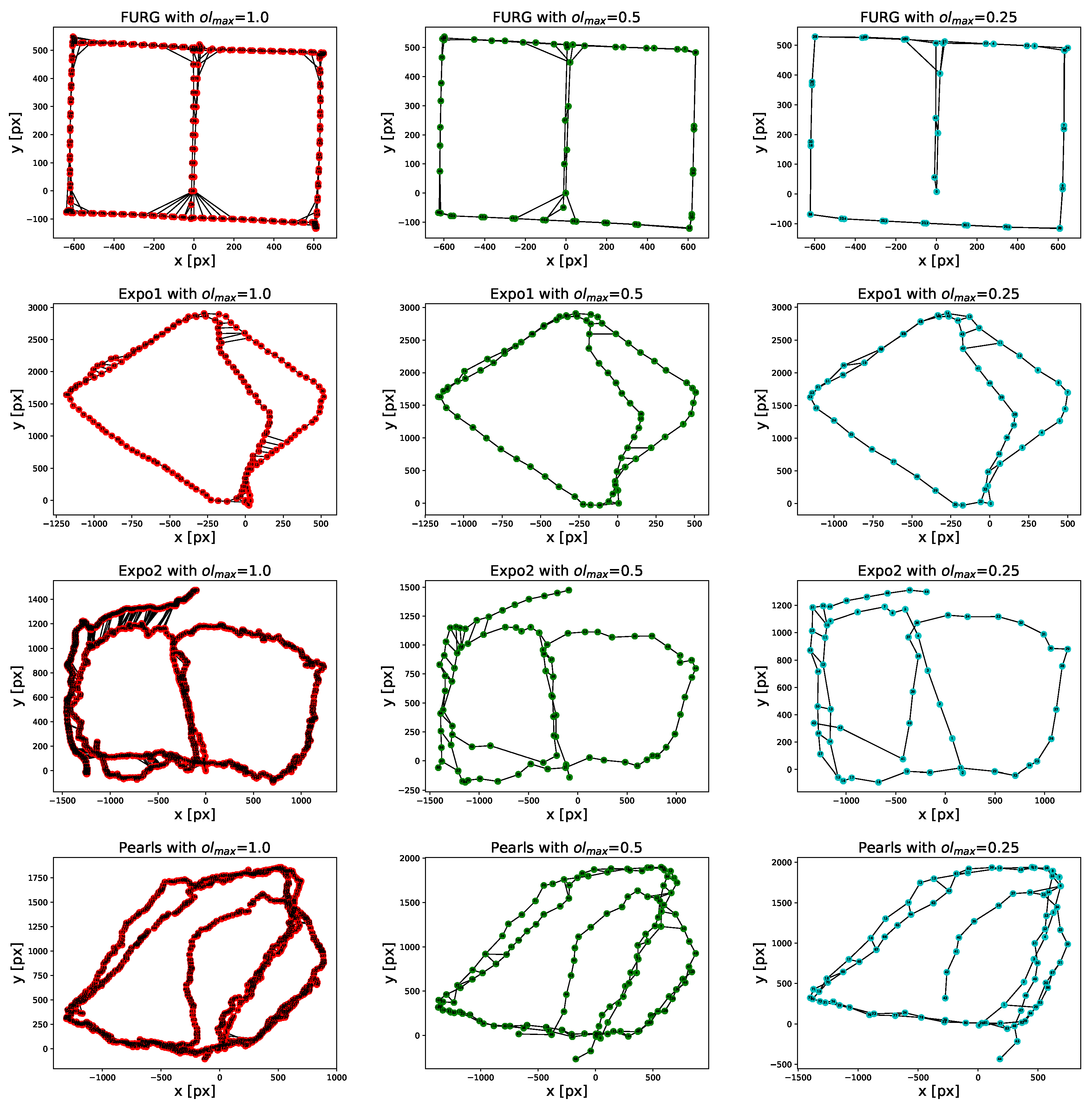
The proposed method has been evaluated with regard to the Precision-Recall ability to recognize previously visited places when using images captured by different agents and when varying the keyframe selection criteria. As presented in the results, the proposed approach manages those factors by striking a compromise between the Precision-Recall and the number of keyframes added to the map. After, we compared the spatial structure of the map obtained after reducing the number of keyframes. We observed that there is no significant difference between the spatial structures when our method uses fewer images than those contained in the original dataset.

In terms of future work, we are interested in testing other types of local features, distinctive enough to require only a few of them, thereby, improving the scalability of the proposed approach. In particular, we are interested in testing the use of features obtained using deep convolutional neural networks as these have shown promising results in matching visual patterns.

References

1. Bosch, A.; Zisserman, A.; Munoz, X. Representing shape with a spatial pyramid kernel. In Proceedings of the 6th ACM International Conference on Image And Video Retrieval, Amsterdam, The Netherlands, 9–11 July 2017; ACM: New York, NY, USA, 2007; pp. 401–408. [Google Scholar]
2. Bay, H.; Ess, A.; Tuytelaars, T.; Gool, L.V. Speeded-Up Robust Features (SURF). Comput. Vis. Image Underst. 2008, 110, 346–359. [Google Scholar] [CrossRef] [Green Version]
3. Cummins, M.; Newman, P. FAB-MAP: Probabilistic localization and mapping in the space of appearance. Int. J. Robot. Res. 2008, 27, 647–665. [Google Scholar] [CrossRef]
4. Csurka, G.; Dance, C.; Fan, L.; Willamowski, J.; Bray, C. Visual categorization with bags of keypoints. In Workshop on Statistical Learning in Computer Vision, ECCV; Springer: Berlin/Heidelberg, Germany, 2004; Volume 1, pp. 1–2. [Google Scholar]
5. Angeli, A.; Filliat, D.; Doncieux, S.; Meyer, J.A. Fast and Incremental Method for Loop-Closure Detection Using Bags of Visual Words. IEEE Trans. Robot. 2008, 24, 1027–1037. [Google Scholar] [CrossRef] [Green Version]
6. Angeli, A.; Doncieux, S.; Meyer, J.A.; Filliat, D. Visual topological SLAM and global localization. In Proceedings of the 2009 IEEE International Conference on Robotics and Automation, Kobe, Japan, 12–17 May 2009; pp. 4300–4305. [Google Scholar] [CrossRef]
7. Rublee, E.; Rabaud, V.; Konolige, K.; Bradski, G. ORB: An efficient alternative to SIFT or SURF. In Proceedings of the 2011 International Conference on Computer Vision, Barcelona, Spain, 6–13 November 2011; pp. 2564–2571. [Google Scholar] [CrossRef]
8. Garcia-Fidalgo, E.; Ortiz, A. Vision-based topological mapping and localization by means of local invariant features and map refinement. Robotica 2015, 33, 1446–1470. [Google Scholar] [CrossRef]
9. Lowe, D.G. Object recognition from local scale-invariant features. In Proceedings of the Seventh IEEE International Conference On Computer Vision, Kerkyra, Greece, 20–27 September 1999; Volume 2, pp. 1150–1157. [Google Scholar]
10. Milford, M.J.; Wyeth, G.F. Mapping a suburb with a single camera using a biologically inspired SLAM system. IEEE Trans. Robot. 2008, 24, 1038–1053. [Google Scholar] [CrossRef]
11. Milford, M.; Wyeth, G. Persistent navigation and mapping using a biologically inspired SLAM system. Int. J. Robot. Res. 2010, 29, 1131–1153. [Google Scholar] [CrossRef]
12. Garcia-Fidalgo, E.; Ortiz, A. Hierarchical Place Recognition for Topological Mapping. IEEE Trans. Robot. 2017, 33, 1061–1074. [Google Scholar] [CrossRef]
13. Rosten, E.; Drummond, T. Machine learning for high-speed corner detection. In Computer Vision–ECCV 2006; Springer: Berlin/Heidelberg, Germany, 2006; pp. 430–443. [Google Scholar]
14. Sermanet, P.; Eigen, D.; Zhang, X.; Mathieu, M.; Fergus, R.; LeCun, Y. Overfeat: Integrated recognition, localization and detection using convolutional networks. arXiv, 2013; arXiv:1312.6229. [Google Scholar]
15. Chen, Z.; Lam, O.; Jacobson, A.; Milford, M. Convolutional neural network-based place recognition. In Proceedings of the Australian Conference on Robotics and Automation, Victoria, Australia, 2–4 December 2014. [Google Scholar]
16. Sünderhauf, N.; Shirazi, S.; Dayoub, F.; Upcroft, B.; Milford, M. On the performance of convnet features for place recognition. In Proceedings of the 2015 IEEE/RSJ International Conference on Intelligent Robots and Systems (IROS), Hamburg, Germany, 28 September–2 October 2015; pp. 4297–4304. [Google Scholar]
17. Krizhevsky, A.; Sutskever, I.; Hinton, G.E. Imagenet classification with deep convolutional neural networks. In Advances in Neural Information Processing Systems; Curran Associates: Red Hook, NY, USA, 2012; pp. 1097–1105. [Google Scholar]
18. Milford, M.J.; Wyeth, G.F. SeqSLAM: Visual route-based navigation for sunny summer days and stormy winter nights. In Proceedings of the 2012 IEEE International Conference on Robotics and Automation, Saint Paul, MN, USA, 14–18 May 2012; pp. 1643–1649. [Google Scholar] [CrossRef]
19. Ouerghi, S.; Boutteau, R.; Savatier, X.; Tlili, F. Visual Odometry and Place Recognition Fusion for Vehicle Position Tracking in Urban Environments. Sensors 2018, 18, 939. [Google Scholar] [CrossRef]
20. Liu, Y.; Zhang, H. Towards improving the efficiency of sequence-based SLAM. In Proceedings of the 2013 IEEE International Conference on Mechatronics and Automation (ICMA), Takamatsu, Japan, 4–7 August 2013; pp. 1261–1266. [Google Scholar]
21. Siam, S.M.; Zhang, H. Fast-seqslam: A fast appearance based place recognition algorithm. In Proceedings of the 2017 IEEE International Conference on Robotics and Automation (ICRA), Singapore, 29 May–3 June 2017; pp. 5702–5708. [Google Scholar]
22. Nicosevici, T.; Garcia, R. Automatic Visual Bag-of-Words for Online Robot Navigation and Mapping. IEEE Trans. Robot. 2012, 28, 886–898. [Google Scholar] [CrossRef]
23. Maldonado-Ramírez, A.; Torres-Méndez, L.A. A Discrete Bayes Filter for visual loop-closing in image sequences of coral reef explorations taken by humans and AUVs. In Proceedings of the OCEANS 2017, Anchorage, AK, USA, 18–21 September 2017; pp. 1–5. [Google Scholar]
24. Guth, F.; Silveira, L.; Botelho, S.; Drews, P.; Ballester, P. Underwater SLAM: Challenges, state of the art, algorithms and a new biologically-inspired approach. In Proceedings of the 5th IEEE RAS/EMBS International Conference on Biomedical Robotics and Biomechatronics, Sao Paulo, Brazil, 12–15 August 2014; pp. 981–986. [Google Scholar] [CrossRef]
25. Silveira, L.; Guth, F.; Drews-Jr, P.; Ballester, P.; Machado, M.; Codevilla, F.; Duarte-Filho, N.; Botelho, S. An Open-source Bio-inspired Solution to Underwater SLAM. IFAC-PapersOnLine 2015, 48, 212–217. [Google Scholar] [CrossRef]
26. Rahman, S.; Li, A.Q.; Rekleitis, I. Sonar Visual Inertial SLAM of Underwater Structures. In Proceedings of the 2018 IEEE International Conference on Robotics and Automation (ICRA), Brisbane, Australia, 21–25 May 2018; pp. 1–7. [Google Scholar]
27. Leutenegger, S.; Lynen, S.; Bosse, M.; Siegwart, R.; Furgale, P. Keyframe-based visual–inertial odometry using nonlinear optimization. Int. J. Robot. Res. 2015, 34, 314–334. [Google Scholar] [CrossRef]
28. Campos, R.; Gracias, N.; Ridao, P. Underwater Multi-Vehicle Trajectory Alignment and Mapping Using Acoustic and Optical Constraints. Sensors 2016, 16, 387. [Google Scholar] [CrossRef] [PubMed]
29. Ruiz, J.J.; Caballero, F.; Merino, L. MGRAPH: A Multigraph Homography Method to Generate Incremental Mosaics in Real-Time From UAV Swarms. IEEE Robot. Autom. Lett. 2018, 3, 2838–2845. [Google Scholar] [CrossRef]
30. Elibol, A.; Kim, J.; Gracias, N.; Garcia, R. Efficient image mosaicing for multi-robot visual underwater mapping. Pattern Recognit. Lett. 2014, 46, 20–26. [Google Scholar] [CrossRef]
31. Bresenham, J.E. Algorithm for computer control of a digital plotter. IBM Syst. J. 1965, 4, 25–30. [Google Scholar] [CrossRef]
32. Duda, R.O.; Hart, P.E. Use of the Hough transformation to detect lines and curves in pictures. Commun. ACM 1972, 15, 11–15. [Google Scholar] [CrossRef] [Green Version]
33. Matas, J.; Galambos, C.; Kittler, J. Robust detection of lines using the progressive probabilistic hough transform. Comput. Vis. Image Underst. 2000, 78, 119–137. [Google Scholar] [CrossRef]
34. Shkurti, F.; Rekleitis, I.; Dudek, G. Feature Tracking Evaluation for Pose Estimation in Underwater Environments. In Proceedings of the 2011 Canadian Conference on Computer and Robot Vision, St. Johns, NL, Canada, 25–27 May 2011; pp. 160–167. [Google Scholar] [CrossRef]
35. Muja, M.; Lowe, D.G. Fast Approximate Nearest Neighbors with Automatic Algorithm Configuration. VISAPP 2009, 2, 2. [Google Scholar]
36. Naseer, T.; Spinello, L.; Burgard, W.; Stachniss, C. Robust Visual Robot Localization Across Seasons Using Network Flows. In Proceedings of the Twenty-Eighth AAAI Conference on Artificial Intelligence (AAAI’14); AAAI Press: Palo Alto, CA, USA, 2014; pp. 2564–2570. [Google Scholar]
37. Vysotska, O.; Stachniss, C. Lazy Data Association for Image Sequences Matching Under Substantial Appearance Changes. IEEE Robot. Autom. Lett. 2016, 1, 213–220. [Google Scholar] [CrossRef]
38. Grisetti, G.; Kummerle, R.; Stachniss, C.; Burgard, W. A Tutorial on Graph-Based SLAM. IEEE Intell. Transp. Syst. Mag. 2010, 2, 31–43. [Google Scholar] [CrossRef]
39. Cummins, M.; Newman, P. Appearance-only SLAM at large scale with FAB-MAP 2.0. Int. J. Robot. Res. 2011, 30, 1100–1123. [Google Scholar] [CrossRef]
40. Duarte, A.C.; Zaffari, G.B.; da Rosa, R.T.S.; Longaray, L.M.; Drews, P.; Botelho, S.S.C. Towards comparison of underwater SLAM methods: An open dataset collection. In Proceedings of the OCEANS 2016 MTS/IEEE Monterey, Monterey, CA, USA, 19–23 September 2016; pp. 1–5. [Google Scholar] [CrossRef]
41. Georgiades, C.; German, A.; Hogue, A.; Liu, H.; Prahacs, C.; Ripsman, A.; Sim, R.; Torres, L.A.; Zhang, P.; Buehler, M.; Dudek, G.; Jenkin, M.; Milios, E. AQUA: An aquatic walking robot. In Proceedings of the 2004 IEEE/RSJ International Conference on Intelligent Robots and Systems (IROS), Sendai, Japan, 28 September–2 October 2004; Volume 4, pp. 3525–3531. [Google Scholar] [CrossRef]
42. Dudek, G.; Jenkin, M.; Prahacs, C.; Hogue, A.; Sattar, J.; Giguere, P.; German, A.; Liu, H.; Saunderson, S.; Ripsman, A.; et al. A visually guided swimming robot. In Proceedings of the 2005 IEEE/RSJ International Conference on Intelligent Robots and Systems (IROS 2005), Edmonton, AB, Canada, 2–6 August 2005; pp. 3604–3609. [Google Scholar]
43. Glover, A.; Maddern, W.; Warren, M.; Reid, S.; Milford, M.; Wyeth, G. OpenFABMAP: An open source toolbox for appearance-based loop closure detection. In Proceedings of the 2012 IEEE International Conference on Robotics and Automation (ICRA), Saint Paul, MN, USA, 14–18 May 2012; pp. 4730–4735. [Google Scholar]
Figure 1. General overview of the proposed approach.
Applsci 09 00261 g001
Figure 2. Example of the overlap calculation. Given two images I a and I b , the visual features between both images are matched. From those matches, a rigid transformation A a b is obtained. After that, we can calculate the intersection between both frames and its area.
Applsci 09 00261 g002
Figure 3. Comparison of a similarity matrix computed by matching directly the visual features and using the voting scheme propose in this work. Each entry ( i , j ) in this matrix indicates the similarity between image i and j. The darker an entry is, the more similar the associated images are. The main diagonals were eliminated from these matrices as they only indicate that the same image is similar to itself.
Applsci 09 00261 g003
Figure 4. Calculation of the base lines. The Bresenham algorithm is applied to every pair of points defined by the central point (blue) and all the points in the grid’s perimeter (yellow).
Applsci 09 00261 g004
Figure 5. Given a similarity matrix S ¯ , we look for the starting points with scores greater than the threshold μ in the last row. Then, we evaluate the score for every predefined line in C translated to each starting point ( ( i s p k , j s p k ) ). The winning sequence c is the one with highest score from all sequences. In this example is the matching sequence starts in point 2.
Applsci 09 00261 g005
Figure 6. Comparison of a topological map with and without pose optimization.
Applsci 09 00261 g006
Figure 7. Example of images taken from the same place but at different distances from the scene.
Applsci 09 00261 g007
Figure 8. Examples of the images contained in each dataset. In the case of Pearls and Expo2 dataset we show images from the same place taken by the different agents (in the same row).
Applsci 09 00261 g008
Figure 9. Precision-Recall curves obtained with o l m a x = 1.0 . This means that all the images in each dataset are utilized. A method is not shown in a plot when it was not able to recognize previously seen places.
Applsci 09 00261 g009
Figure 10. Precision-Recall curves obtained with o l m a x = 0.5 . A method is not shown in a plot when it was not able to recognize previously seen places.
Applsci 09 00261 g010aApplsci 09 00261 g010b
Figure 11. Precision-Recall curves obtained with o l m a x = 0.25 . A method is not shown in a plot when it was not able to recognize previously seen places.
Applsci 09 00261 g011
Figure 12. Examples of recognized places from images taken from different agents. (a) In this example the image taken by the underwater robot is from the same place than the one taken by a diver but rotated approximately 90° to the right. (b) The same place is captured in both images but the one captured by the robot is closer to the coral reef than the one captured by the diver. Moreover, the image captured by the robot is more illuminated. (c) These images were taken from the same place but the one captured by the second diver is closer to the coral reef and rotated approximately 90° to the left with respect to the one captured by the first diver. In addition to that, the second one is more bluish than the first one. (d) In this case the image captured by the second diver is closer to the coral reef and rotated to the approximately 90° left with respect to the one captured by the first diver.
Applsci 09 00261 g012
Figure 13. Obtained graphs from applying our method to each dataset varying the overlap factor o l m a x .
Applsci 09 00261 g013
Figure 14. Obtained mosaics from applying our method to each dataset.
Applsci 09 00261 g014