Investigation on the Potential to Integrate Different Artificial Intelligence Models with Metaheuristic Algorithms for Improving River Suspended Sediment Predictions


 ,
, 

Abstract
1. Introduction
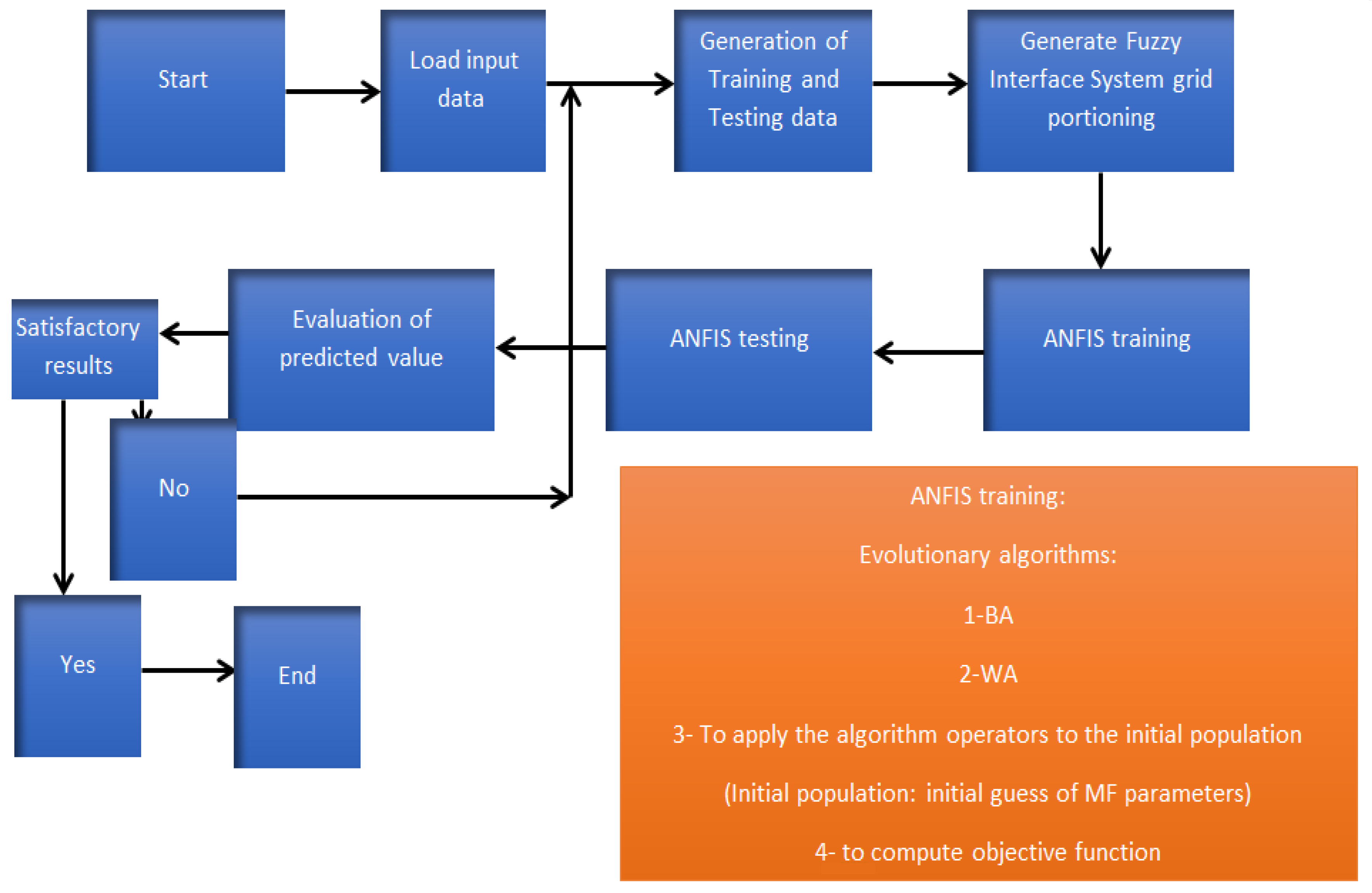
- To improve ANFIS and MFNN model efficiency by applying new optimization algorithms. These algorithms are used to obtain the best ANFIS and MFNN structures and parameters;
- To predict monthly sediment load by applying improved ANFIS and MFNN models;
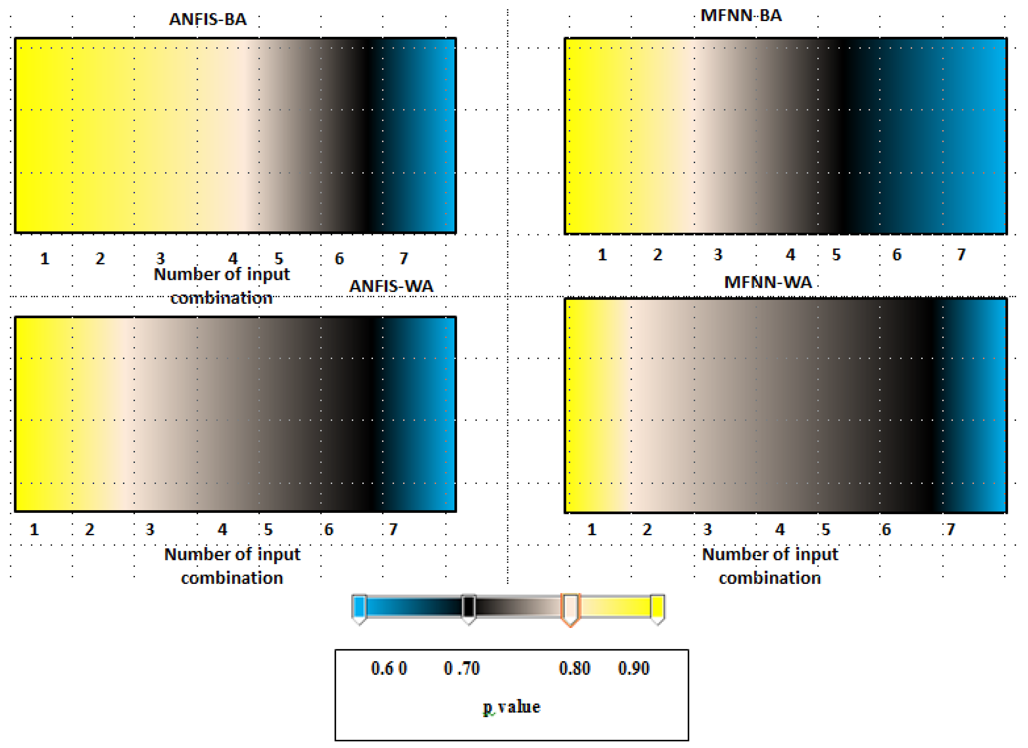
- To examine the uncertainty of the predictions; and
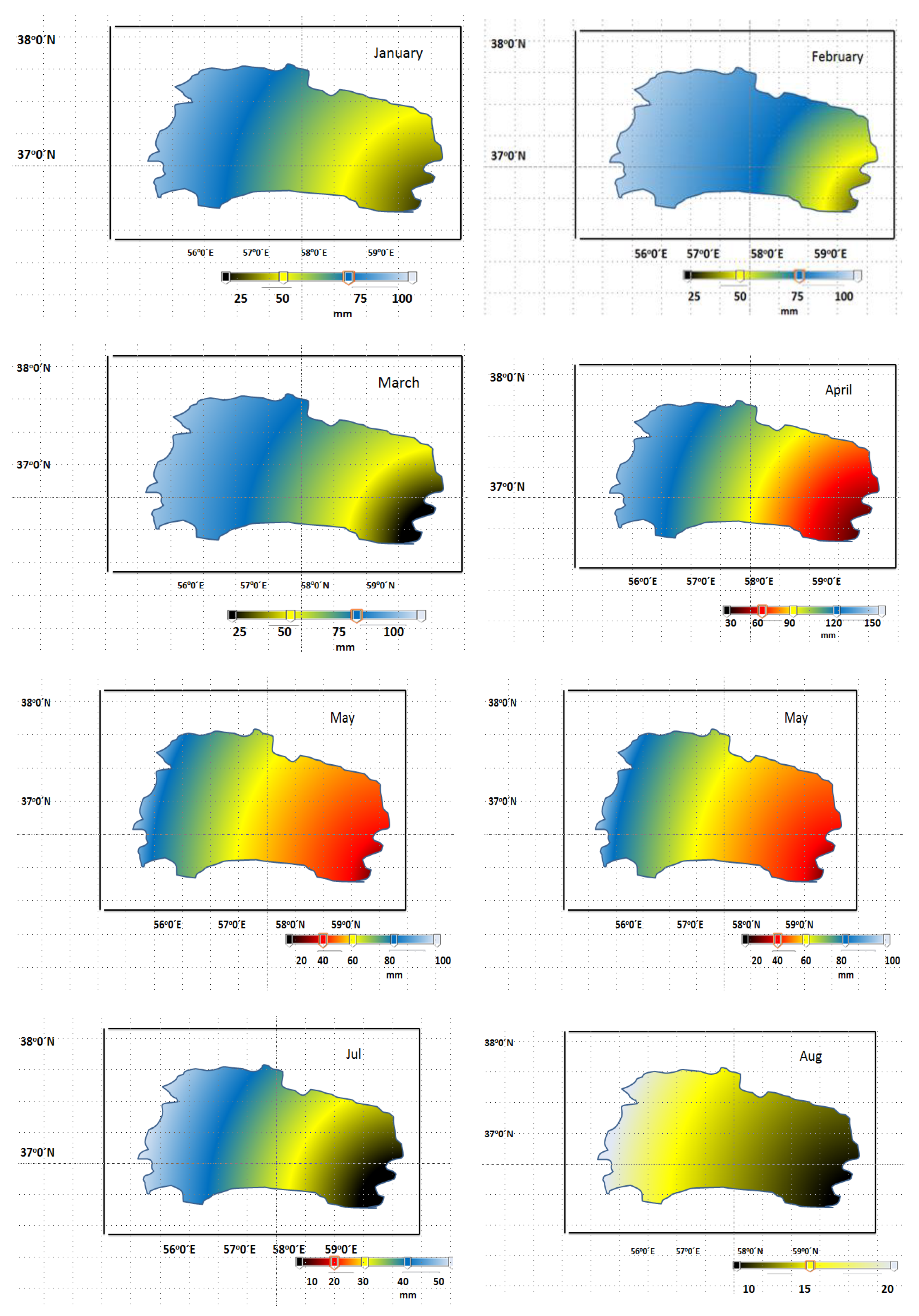
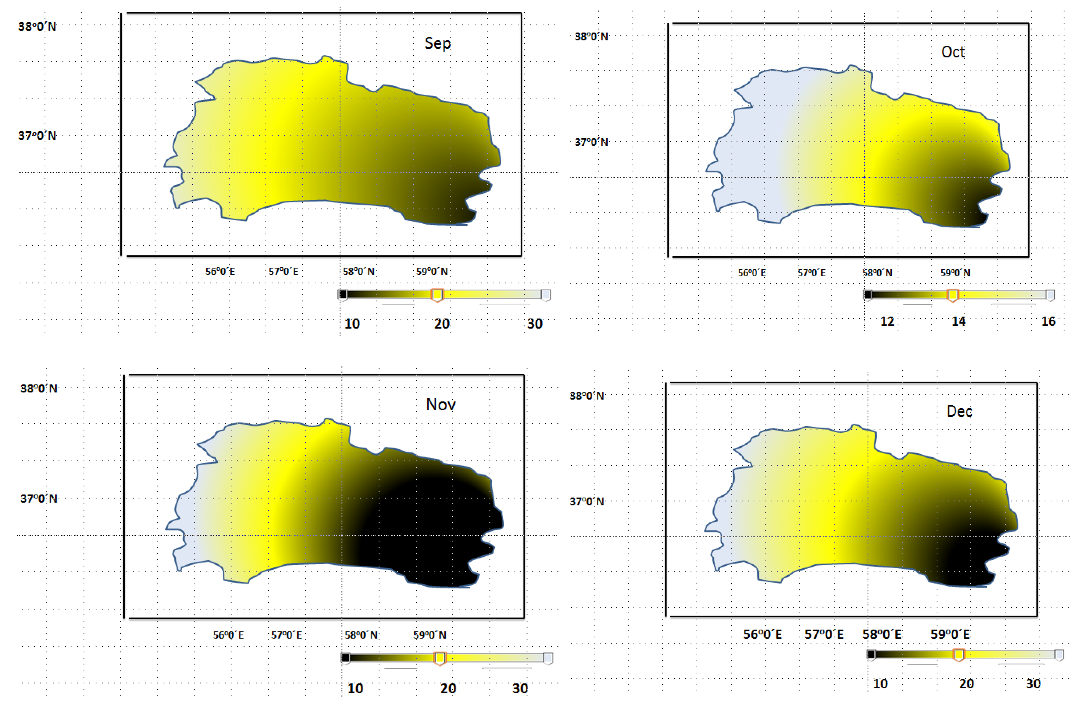
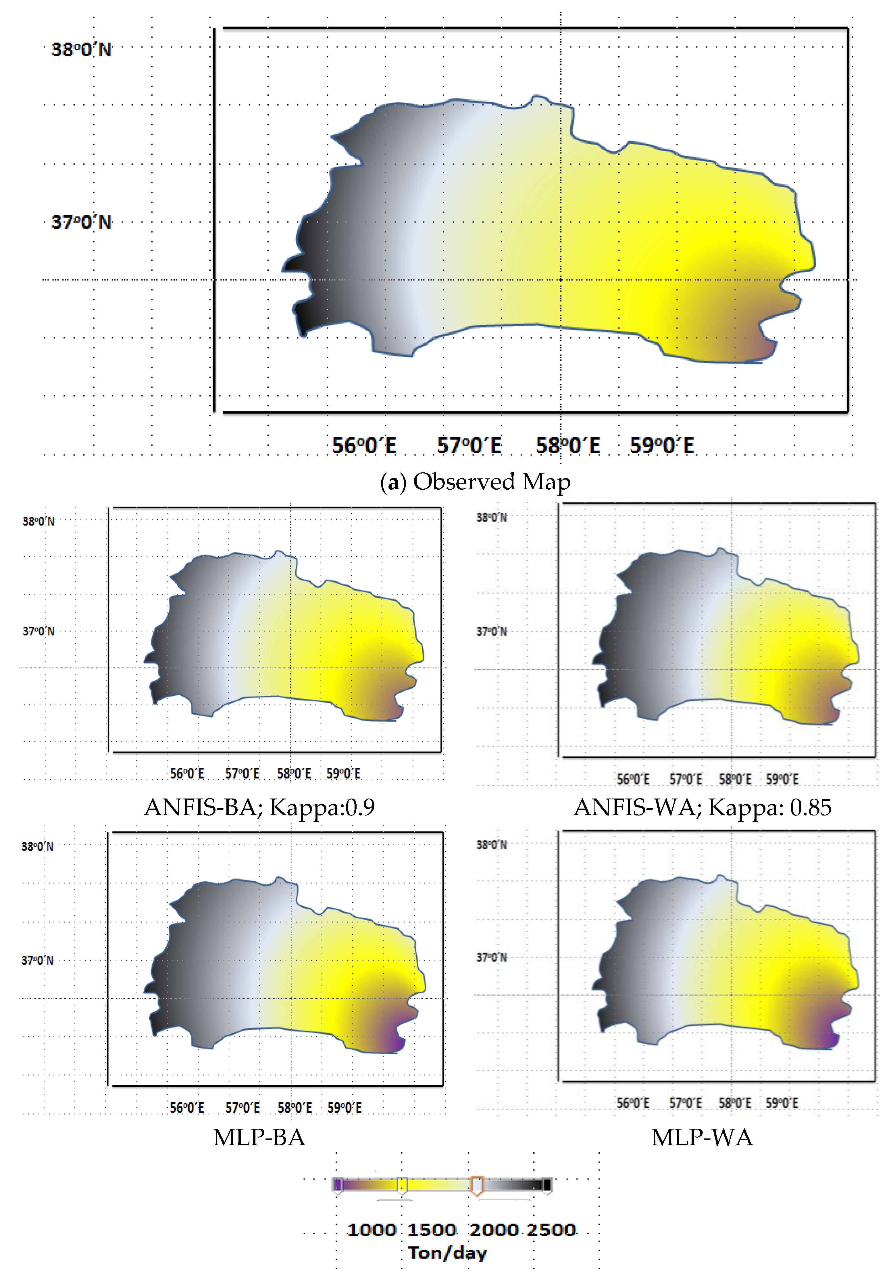
- To obtain a sediment map of the case study.
2. Literature Review
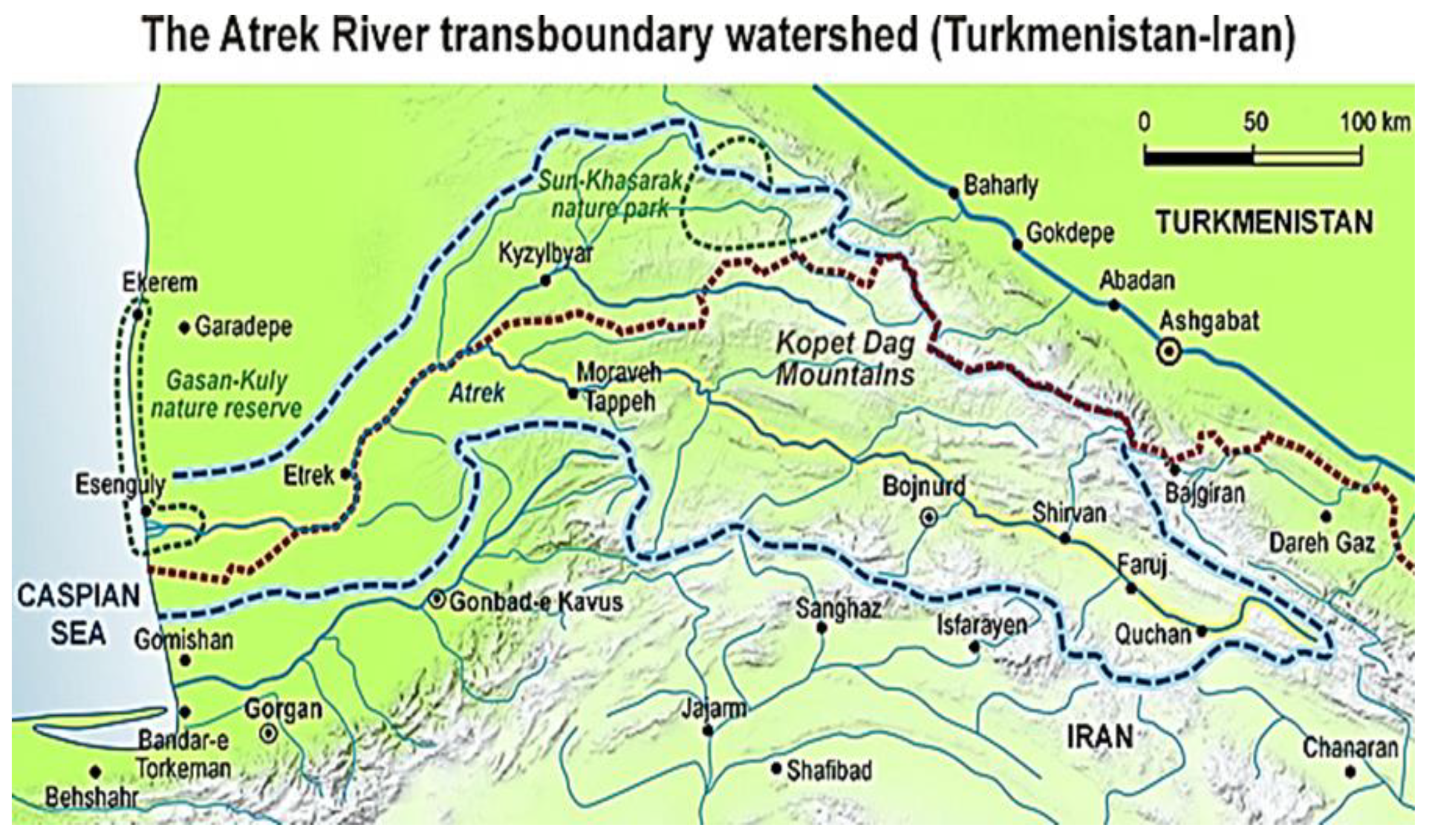
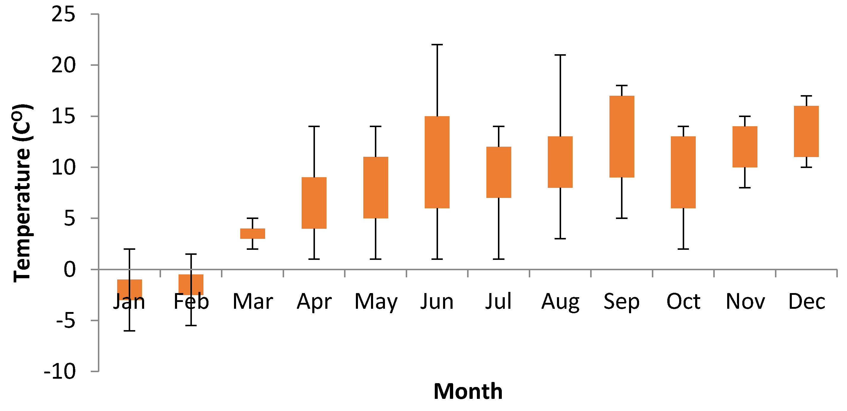
2.1. Case Study
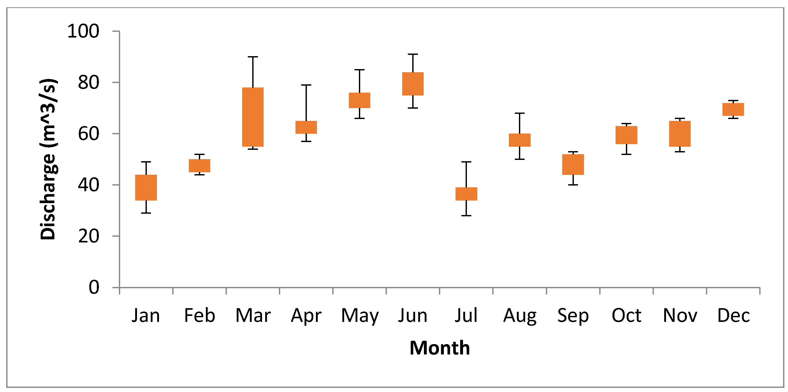
2.2. Data and Parameters Applied in Suspended Sediment Load (SSL) Prediction
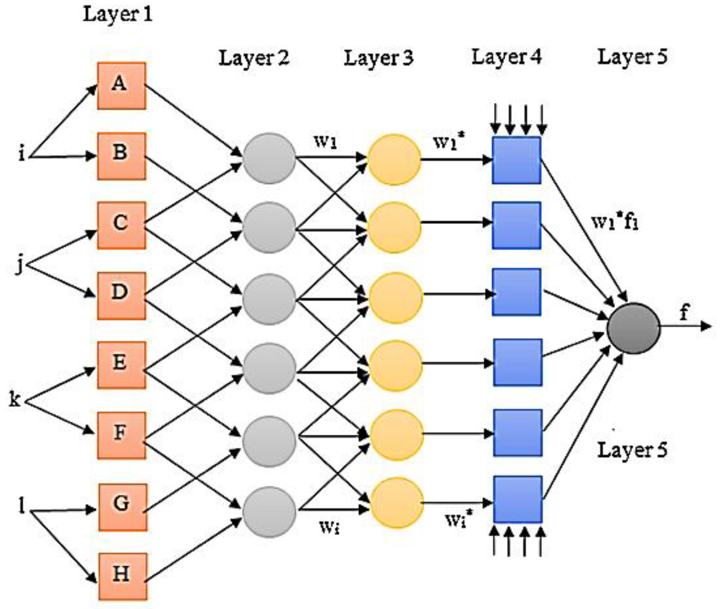
2.3. Adaptive Neuro Fuzzy System (ANFIS) Method
- The first layer calculates the membership degree. Each node produces a membership degree. The fuzzy sets apply membership functions [29].where and y are outputs, Ai and Bi are linguistic labels, and and are the degree of membership function for Ai and Bi, respectively.
- The output of the second layer (fire strengths) is computed based on the computed membership degrees. In fact, membership functions of the previous layer are compounded together to generate the firing strengths.where is the output of this layer called fire strength.
- The firing strengths are normalized in this level. The contribution of the firing strengths is computed by the constant nodes:
- In this layer, consequent parameters are used to determine the proportion of the ith rule to the overall outcomes:where pi, qi, and ri are consequent parameters.
- This layer uses summation of input signals to obtain the overall output.
2.4. Feed-Forward Neural Network (FNN)
2.5. ANFIS and Multilayer FNN (MFNN) Models and Optimization Algorithms
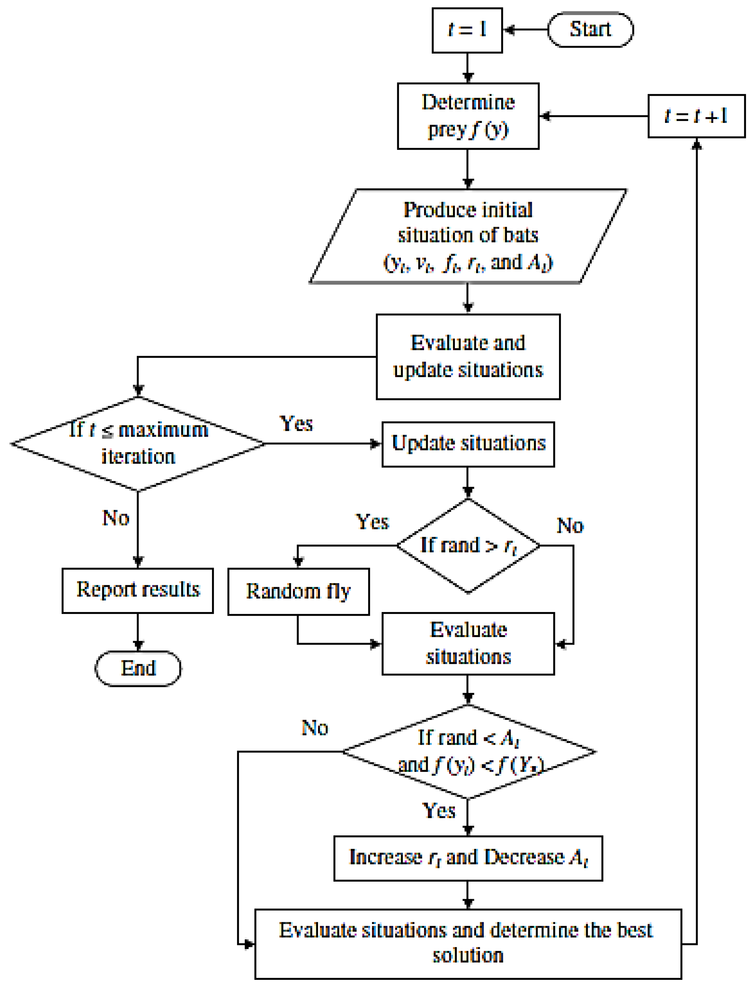
- Bat algorithm (BA): BA is an optimization algorithm that acts based on echolocation characteristics. Each of the flying bats has a random velocity and flies at random positions. When it is searching for prey, its loudness, frequency, and pulsation rates are widely varied. A local random walk is used to increase the search ability [26]. The velocity and position components are used to obtain the optimal solutions. Each position is a candidate solution. Thus, the best position is the best solution while the algorithm should avoid trapping in the local optimums (Figure 6). In fact, bats generate sounds that are returned from the surroundings. They can differentiate an obstacle from prey based on returned frequencies [26].The velocity, frequency, and position are defined as:where is frequency, is minimum frequency, is maximum frequency, is velocity, is position, and is the best position.Equation (9) defines the local search applying a random walk [30]:where is loudness and is a random value. The pulsation and loudness rate are varied during computational levels. If a bat finds its prey, the pulsation (rl) and loudness rate have an increasing and decreasing trend, respectively. The quality solutions are identified by the objective function computation (Figure 6).
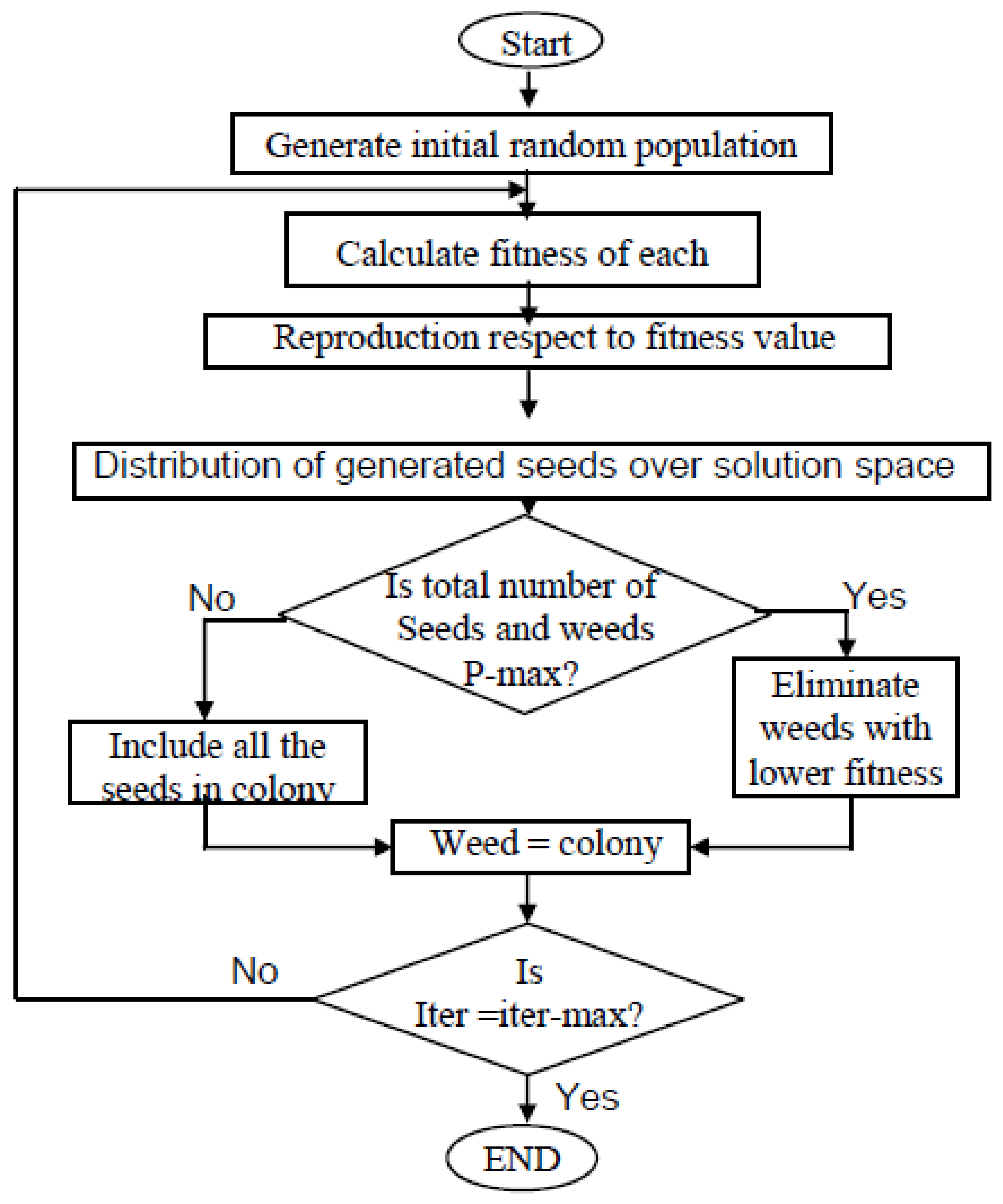
- Weed algorithm (WA): Weeds attempt to find the best growth position. Among all the characteristics of this optimization algorithm, its easy structure, high accuracy, and few random parameters make it useful for practice in optimization problems.
- Initialization: The initial population is distributed randomly in a d dimensional problem space. The locations of weeds are considered as the decision-making components.
- Reproduction: The weeds generate a particular number of seeds. The number of seeds varies from Smin (minimum number of seeds) to Smax (maximum number of seeds). The number of seeds is Smax if a weed has the best objective function value. Although the quality of some weeds is not good, the reproduction process allows them to have a chance again for continuation of life. This issue is important because some of them may have important information. If they do not have another chance, important information is eliminated from the algorithm cycle.
- Competitive level: The combination of weeds produces the next weed generation. If the population exceeds a threshold, the weeds with low quality are eliminated compared to weeds with high quality.
- Termination level: The algorithm finishes when the number of algorithm levels of iteration (Iter) reaches the maximum number of iterations (iter-max), which has been proposed to be 1000 iterations. (Figure 7).
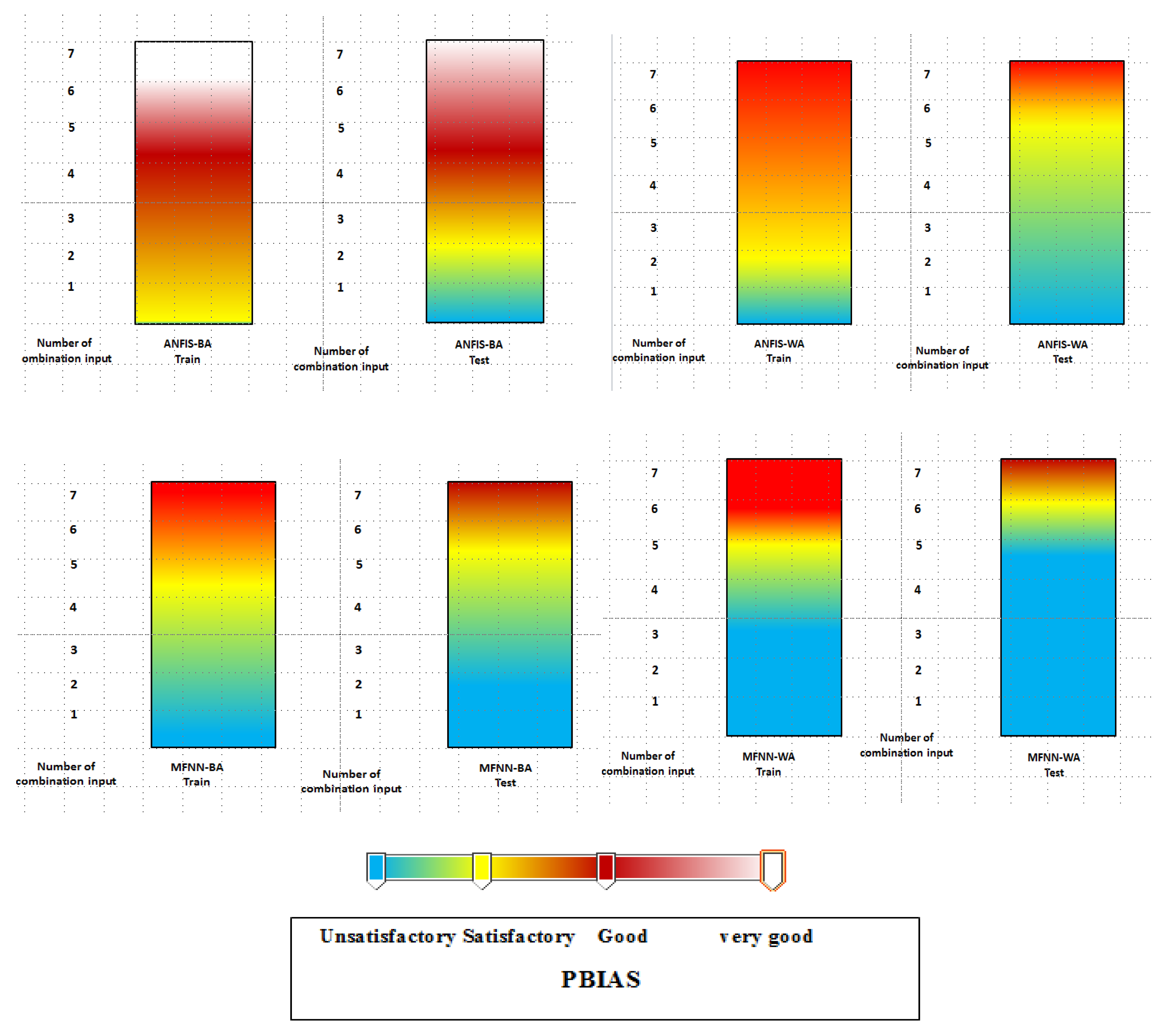
- Percent bias:
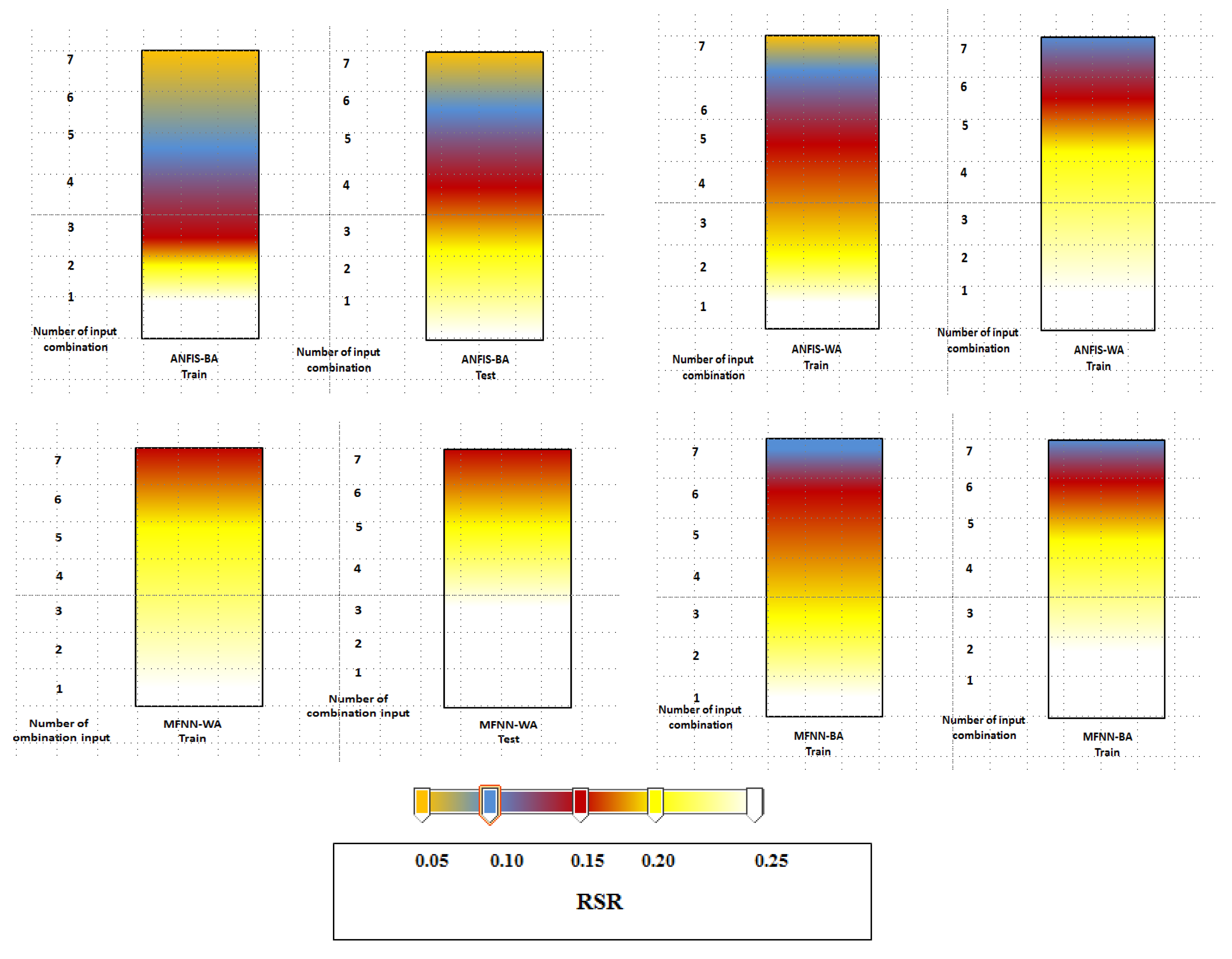
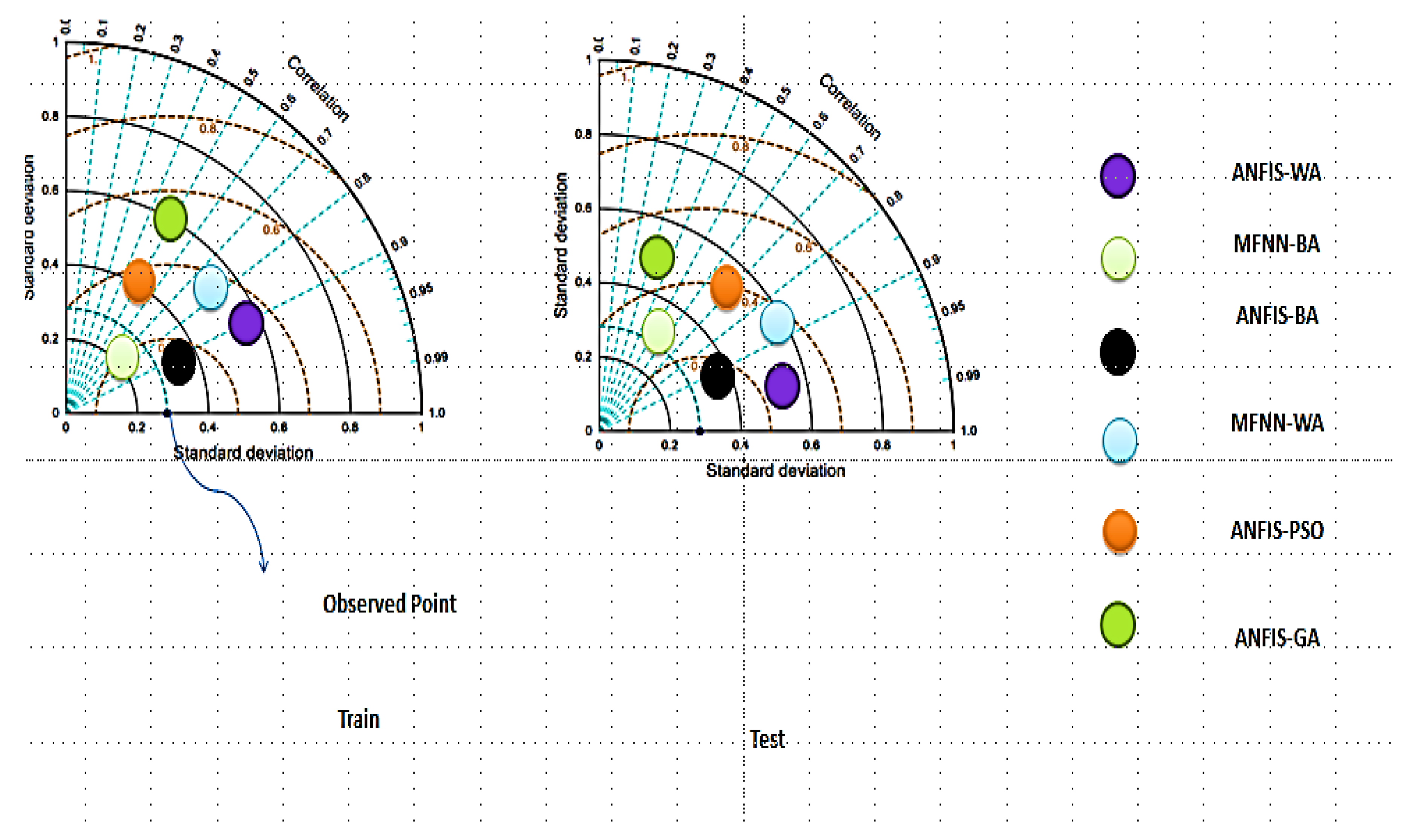
- Standard deviation of RMSE observations
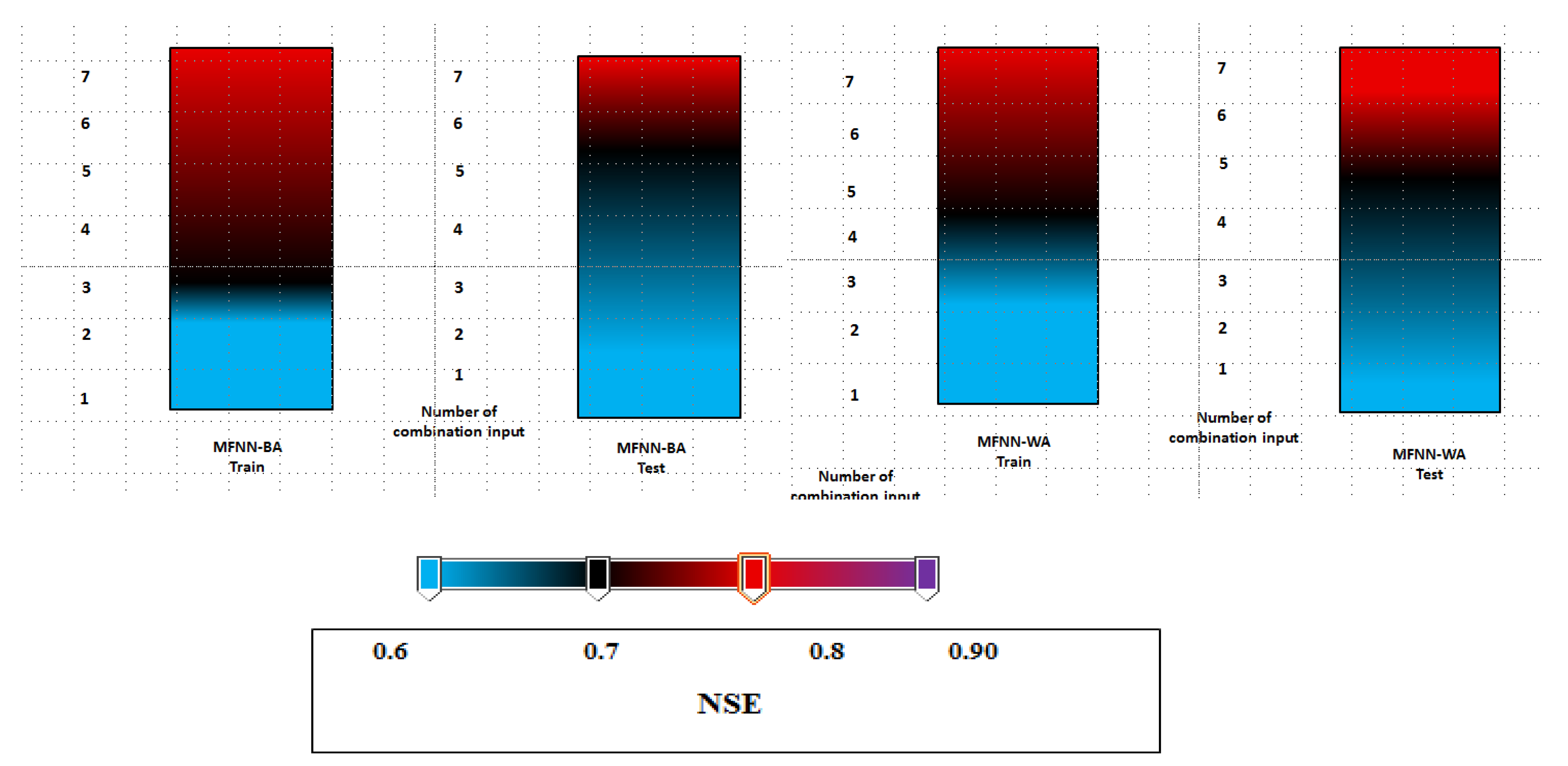
- Nash–Sutcliff efficiency
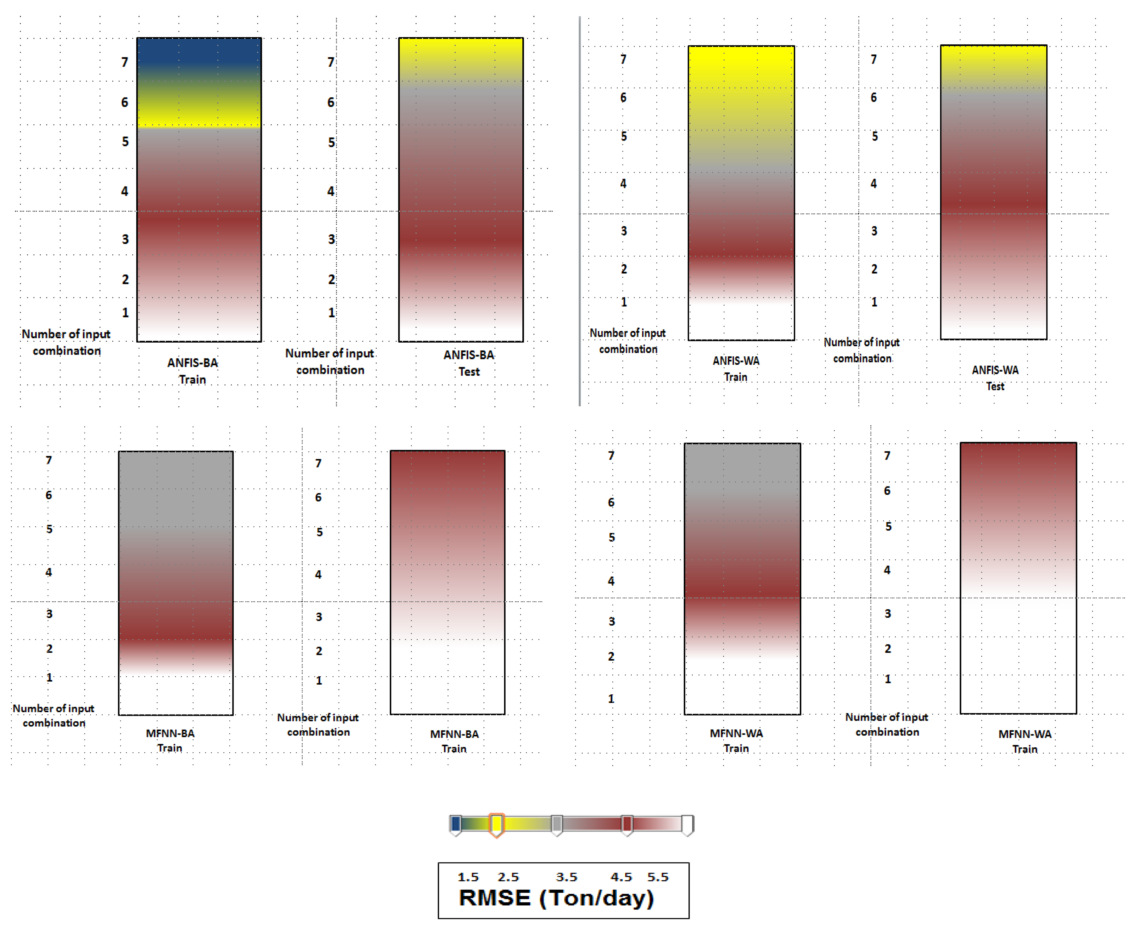
- RMSE (root-mean-square error)is observed data, is simulated data, N is the number of data, and is the average value of the data.
3. Results and Discussion
3.1. Sensitivity Analysis for Optimization Algorithms
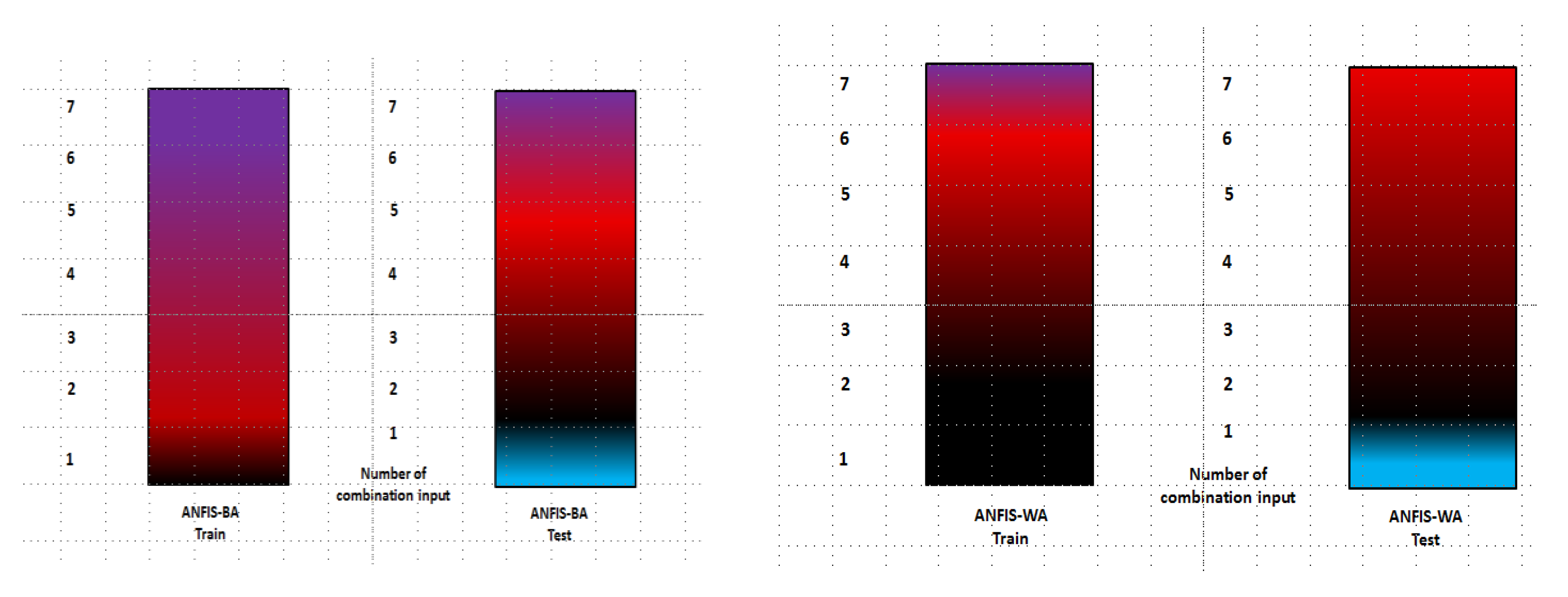
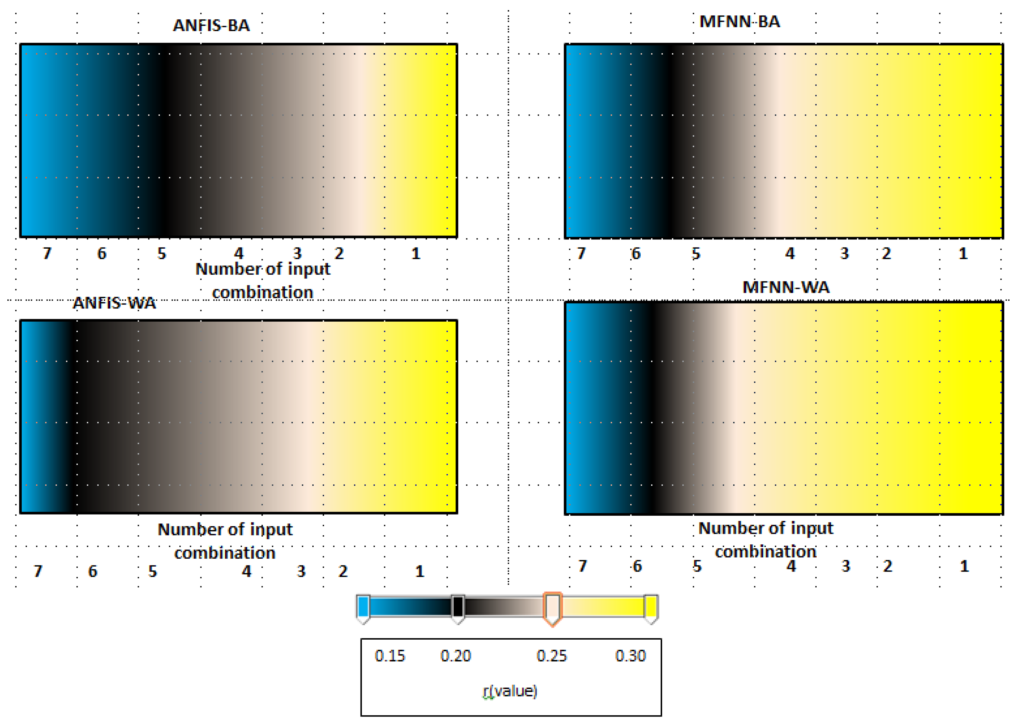
3.2. Performance Index Analysis
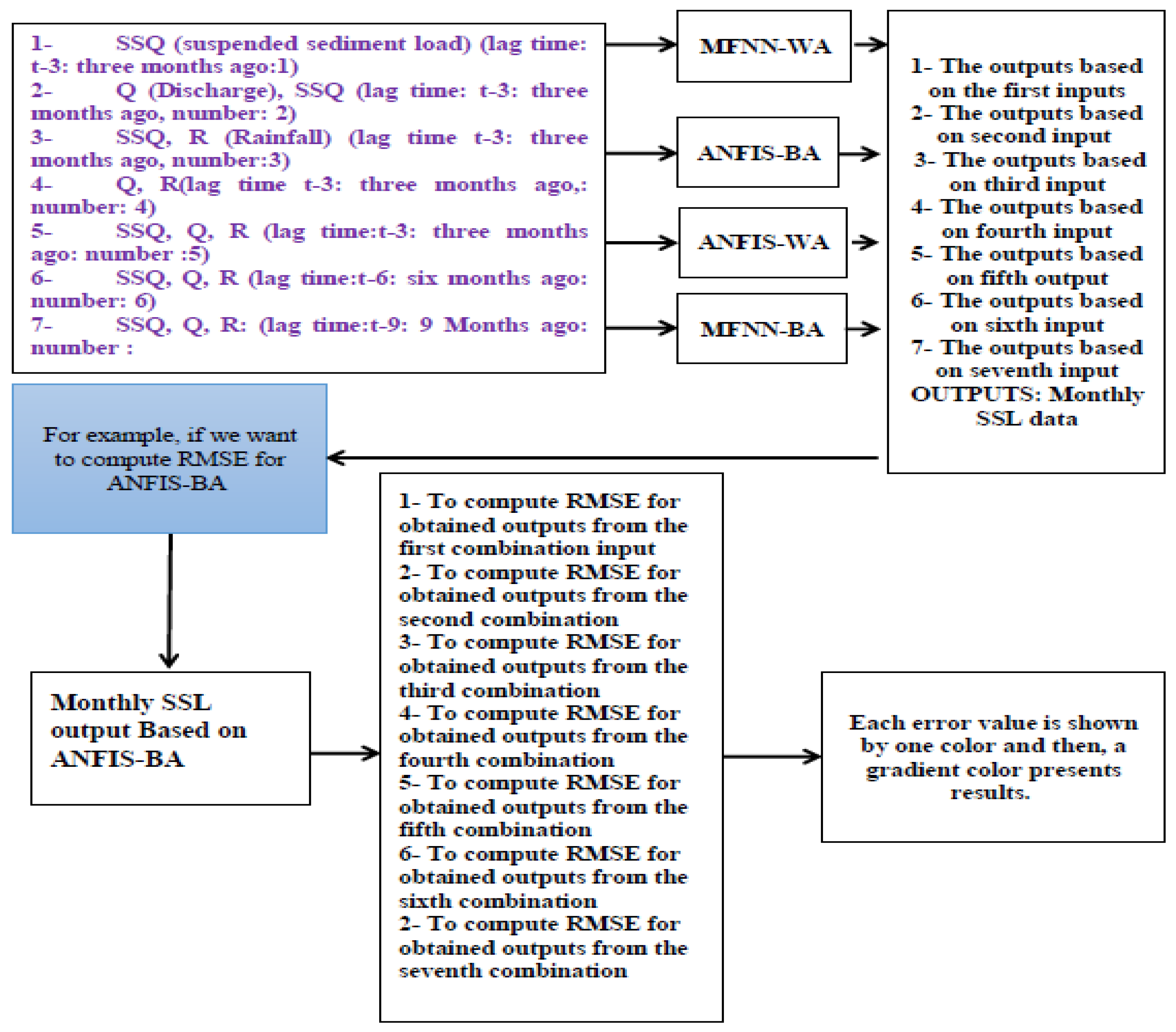
- SSL (suspended sediment load) (lag time t–3: three months ago, number: 1);
- Q (discharge), SSQ (lag time t-3: three months ago, number: 2);
- SSQ, R (rainfall) (lag time t-3: three months ago, number: 3);
- Q, R (lag time t-3: three months ago, number: 4);
- SSL, Q, R (lag time t-3: three months ago, number: 5);
- SSL, Q, R (lag time t-6: 6 months ago, number: 6); and
- SSL, Q, R: (lag time t-9: 9 months ago, number: 7).
3.3. Discussion of Results
4. Conclusions
Author Contributions
Funding
Acknowledgments
Conflicts of Interest
References
- Liu, Q.J.; Zhang, H.Y.; Gao, K.T.; Xu, B.; Wu, J.Z.; Fang, N.F. Time-frequency analysis and simulation of the watershed suspended sediment concentration based on the Hilbert-Huang transform (HHT) and artificial neural network (ANN) methods: A case study in the Loess Plateau of China. Catena 2019, 179, 107–118. [Google Scholar] [CrossRef]
- Sharghi, E.; Nourani, V.; Najafi, H.; Gokcekus, H. Conjunction of a newly proposed emotional ANN (EANN) and wavelet transform for suspended sediment load modeling. Water Supply 2019, 19, 1726–1734. [Google Scholar] [CrossRef]
- Nourani, V.; Molajou, A.; Tajbakhsh, A.D.; Najafi, H. A Wavelet Based Data Mining Technique for Suspended Sediment Load Modeling. Water Resour. Manag. 2019, 33, 1769–1784. [Google Scholar] [CrossRef]
- Abobakr Yahya, A.S.; Ahmed, A.N.; Binti Othman, F.; Ibrahim, R.K.; Afan, H.A.; El-Shafie, A.; Fai, C.M.; Hossain, M.S.; Ehteram, M.; Elshafie, A. Water Quality Prediction Model Based Support Vector Machine Model for Ungauged River Catchment under Dual Scenarios. Water 2019, 11, 1231. [Google Scholar] [CrossRef]
- Tabatabaei, M.; Salehpour Jam, A.; Hosseini, S.A. Suspended sediment load prediction using non-dominated sorting genetic algorithm II. Int. Soil Water Conserv. Res. 2019, 7, 119–129. [Google Scholar] [CrossRef]
- Hassanpour, F.; Sharifazari, S.; Ahmadaali, K.; Mohammadi, S.; Sheikhalipour, Z. Development of the FCM-SVR Hybrid Model for Estimating the Suspended Sediment Load. KSCE J. Civ. Eng. 2019, 23, 2514–2523. [Google Scholar] [CrossRef]
- Rezakazemi, M.; Mosavi, A.; Shirazian, S. ANFIS pattern for molecular membranes separation optimization. J. Mol. Liq. 2019, 274, 470–476. [Google Scholar] [CrossRef]
- Sihag, P.; Tiwari, N.K.; Ranjan, S. Prediction of unsaturated hydraulic conductivity using adaptive neuro- fuzzy inference system (ANFIS). ISH J. Hydraul. Eng. 2017, 25, 132–142. [Google Scholar] [CrossRef]
- Karaboga, D.; Kaya, E. Training ANFIS by Using an Adaptive and Hybrid Artificial Bee Colony Algorithm (aABC) for the Identification of Nonlinear Static Systems. Arab. J. Sci. Eng. 2018, 44, 3531–3547. [Google Scholar] [CrossRef]
- Ho, J.Y.; Afan, H.A.; El-Shafie, A.H.; Koting, S.B.; Mohd, N.S.; Jaafar, W.Z.B.; Lai Sai, H.; Malek, M.A.; Ahmed, A.N.; Mohtar, W.H.M.W.; et al. Towards a time and cost effective approach to water quality index class prediction. J. Hydrol. 2019, 575, 148–165. [Google Scholar] [CrossRef]
- Gao, F.; Wang, Y.; Hu, X. Evaluation of the suitability of Landsat, MERIS, and MODIS for identifying spatial distribution patterns of total suspended matter from a self-organizing map (SOM) perspective. Catena 2019, 172, 699–710. [Google Scholar] [CrossRef]
- Binns, A.D.; Fata, A.; Ferreira da Silva, A.M.; Bonakdari, H.; Gharabaghi, B. Modeling Performance of Sediment Control Wet Ponds at Two Construction Sites in Ontario, Canada. J. Hydraul. Eng. 2019, 145, 5019001. [Google Scholar] [CrossRef]
- Guven, A.; Kişi, Ö. Estimation of Suspended Sediment Yield in Natural Rivers Using Machine-coded Linear Genetic Programming. Water Resour. Manag. 2010, 25, 691–704. [Google Scholar] [CrossRef]
- Kisi, O.; Yaseen, Z.M. The potential of hybrid evolutionary fuzzy intelligence model for suspended sediment concentration prediction. Catena 2019, 174, 11–23. [Google Scholar] [CrossRef]
- Choubin, B.; Darabi, H.; Rahmati, O.; Sajedi-Hosseini, F.; Kløve, B. River suspended sediment modelling using the CART model: A comparative study of machine learning techniques. Sci. Total Environ. 2018, 615, 272–281. [Google Scholar] [CrossRef] [PubMed]
- Kakaei Lafdani, E.; Moghaddam Nia, A.; Ahmadi, A. Daily suspended sediment load prediction using artificial neural networks and support vector machines. J. Hydrol. 2013, 478, 50–62. [Google Scholar] [CrossRef]
- Ebtehaj, I.; Bonakdari, H. Evaluation of Sediment Transport in Sewer using Artificial Neural Network. Eng. Appl. Comput. Fluid Mech. 2013, 7, 382–392. [Google Scholar] [CrossRef]
- Melesse, A.M.; Ahmad, S.; McClain, M.E.; Wang, X.; Lim, Y.H. Suspended sediment load prediction of river systems: An artificial neural network approach. Agric. Water Manag. 2011, 98, 855–866. [Google Scholar] [CrossRef]
- Shiau, J.-T.; Chen, T.-J. Quantile Regression-Based Probabilistic Estimation Scheme for Daily and Annual Suspended Sediment Loads. Water Resour. Manag. 2015, 29, 2805–2818. [Google Scholar] [CrossRef]
- Chen, X.Y.; Chau, K.W. A Hybrid Double Feedforward Neural Network for Suspended Sediment Load Estimation. Water Resour. Manag. 2016, 30, 2179–2194. [Google Scholar] [CrossRef]
- Shamaei, E.; Kaedi, M. Suspended sediment concentration estimation by stacking the genetic programming and neuro-fuzzy predictions. Appl. Soft Comput. 2016, 45, 187–196. [Google Scholar] [CrossRef]
- Buyukyildiz, M.; Kumcu, S.Y. An Estimation of the Suspended Sediment Load Using Adaptive Network Based Fuzzy Inference System, Support Vector Machine and Artificial Neural Network Models. Water Resour. Manag. 2017, 31, 1343–1359. [Google Scholar] [CrossRef]
- Mustafa, M.R.; Rezaur, R.B.; Saiedi, S.; Isa, M.H. River Suspended Sediment Prediction Using Various Multilayer Perceptron Neural Network Training Algorithms—A Case Study in Malaysia. Water Resour. Manag. 2012, 26, 1879–1897. [Google Scholar] [CrossRef]
- Khosravi, K.; Mao, L.; Kisi, O.; Yaseen, Z.M.; Shahid, S. Quantifying hourly suspended sediment load using data mining models: Case study of a glacierized Andean catchment in Chile. J. Hydrol. 2018, 567, 165–179. [Google Scholar] [CrossRef]
- Khan, M.Y.A.; Tian, F.; Hasan, F.; Chakrapani, G.J. Artificial neural network simulation for prediction of suspended sediment concentration in the River Ramganga, Ganges Basin, India. Int. J. Sediment Res. 2019, 34, 95–107. [Google Scholar] [CrossRef]
- Cai, X.; Wang, H.; Cui, Z.; Cai, J.; Xue, Y.; Wang, L. Bat algorithm with triangle-flipping strategy for numerical optimization. Int. J. Mach. Learn. Cybern. 2017, 9, 199–215. [Google Scholar] [CrossRef]
- Biswas, P.; Navaneethkrishnan, B.; Anand, G.; Omkar, S.N. System identification of a small scaled helicopter using simulated annealing algorithm. In Proceedings of the 2018 Indian Control Conference, Kanpur, India, 4–6 January 2018. [Google Scholar]
- Peña-Angulo, D.; Nadal-Romero, E.; González-Hidalgo, J.C.; Albaladejo, J.; Andreu, V.; Bagarello, V.; Barhi, H.; Batalla, R.J.; Bernal, S.; Bienes, R.; et al. Spatial variability of the relationships of runoff and sediment yield with weather types throughout the Mediterranean basin. J. Hydrol. 2019, 571, 390–405. [Google Scholar] [CrossRef]
- Ehteram, M.; Afan, H.A.; Dianatikhah, M.; Ahmed, A.N.; Fai, C.M.; Hossain, M.S.; Allawi, M.F.; Elshafie, A.; Ehteram, M.; Afan, H.A.; et al. Assessing the Predictability of an Improved ANFIS Model for Monthly Streamflow Using Lagged Climate Indices as Predictors. Water 2019, 11, 1130. [Google Scholar] [CrossRef]
- Valikhan-Anaraki, M.; Mousavi, S.-F.; Farzin, S.; Karami, H.; Ehteram, M.; Kisi, O.; Chow, M.F.; Hossain, M.; Hayder, G.; Najah, A.-M.; et al. Development of a Novel Hybrid Optimization Algorithm for Minimizing Irrigation Deficiencies. Sustainability 2019, 11, 2337. [Google Scholar] [CrossRef]
- Yaseen, Z.M.; Ehteram, M.; Sharafati, A.; Shahid, S.; Al-Ansari, N.; El-Shafie, A. The integration of nature-inspired algorithms with Least Square Support Vector regression models: Application to modeling river dissolved oxygen concentration. Water 2018, 10, 1124. [Google Scholar] [CrossRef]
- Ehteram, M.; Ahmed, A.N.; Fai, C.M.; Afan, H.A.; El-Shafie, A. Accuracy Enhancement for Zone Mapping of a Solar Radiation Forecasting Based Multi-Objective Model for Better Management of the Generation of Renewable Energy. Energies 2019, 12, 2730. [Google Scholar] [CrossRef]
- Tariq, Z.; Mahmoud, M.; Abdulraheem, A. Core log integration: A hybrid intelligent data-driven solution to improve elastic parameter prediction. Neural Comput. Appl. 2019. [Google Scholar] [CrossRef]
- Yilmaz, B.; Aras, E.; Nacar, S.; Kankal, M. Estimating suspended sediment load with multivariate adaptive regression spline, teaching-learning based optimization, and artificial bee colony models. Sci. Total Environ. 2018, 639, 826–840. [Google Scholar] [CrossRef] [PubMed]
- Najah, A.-M.; El-Shafie, A.; Karim, O.A. An augmented Wavelet De-noising Technique with Neuro-Fuzzy Inference System for water quality prediction. Int. J. Innov. Comput. Inf. Control 2012, 8, 7055–7082. [Google Scholar]


| Model Simulation | Parameter | Time Lag | Output |
|---|---|---|---|
| Group 1 | SSL | t-3 | Suspended Sediment Load (SSL) (t) |
| Group 2 | Q, SSL | t-3 | SSL (t) |
| Group 3 | SSL, R | t-3 | SSL (t) |
| Group 4 | Q, R | t-3 | SSL (t) |
| Group 5 | SSL, Q, R | t-3 | SSL (t) |
| Group 6 | SSL, Q, R | t-6 | SSL (t) |
| Group 7 | SSL, Q, R | t-9 | SSL (t) |
| SP: Size of Population | Maximum Frequency (MaxF) | Minimum Frequency (MinF) | Maximum Loudness (MaxA) | Minimum Loudness (MinA) |
|---|---|---|---|---|
| 10 | 0.3 | 0.10 | 3 | 1 |
| 30 | 0.5 | 0.20 | 5 | 2 |
| 50 | 0.7 | 0.30 | 7 | 3 |
| 70 | 0.90 | 0.40 | 9 | 4 |
| Mean objective function for the first combination of random parameters: 3.12 ton/month (SP:10, MAXF:0.30, MINF:0.10, MAXA:3 and Min A:1) | ||||
| SP: Size of Population | Maximum Frequency (MAXF) | Minimum Frequency (MinF) | Maximum Loudness (MAXA) | Minimum Loudness (MinA) |
|---|---|---|---|---|
| 10 | 0.3 | 0.10 | 3 | 1 |
| 30 | 0.5 | 0.2 | 5 | 2 |
| 50 | 0.7 | 0.30 | 7 | 3 |
| 70 | 0.90 | 0.40 | 9 | 4 |
| Mean objective function for the first combination of random parameters: 3.02 ton/month (SP:10, MAXF:0.30, MINF:0.10, MAXA:3 and Min A:3) | ||||
| SP: Size of Population | Maximum Frequency (MAXF) | Minimum Frequency (MinF) | Maximum Loudness (MAXA) | Minimum Loudness (MinA) |
|---|---|---|---|---|
| 10 | 0.3 | 0.10 | 3 | 1 |
| 30 | 0.5 | 0.20 | 5 | 2 |
| 50 | 0.7 | 0.30 | 7 | 3 |
| 70 | 0.90 | 0.40 | 9 | 4 |
| Mean objective function for the first combination of random parameters: 2.97 ton/month (SP:10, MAXF:0.30, MINF:0.10, MAXA:5 and Min A:3) | ||||
| SP: Size of Population | Maximum Frequency (MAXF) | Minimum Frequency (MinF) | Maximum Loudness (MAXA) | Minimum Loudness (MinA) |
|---|---|---|---|---|
| 10 | 0.3 | 0.10 | 3 | 1 |
| 30 | 0.5 | 0.20 | 5 | 2 |
| 50 | 0.7 | 0.30 | 7 | 3 |
| 70 | 0.90 | 0.40 | 9 | 4 |
| Mean objective function for the first combination of random parameters: 3.15 ton/month (SP:10, MAXF:0.30, MINF:0.10, MAXA:5 and Min A:7 | ||||
| BA | Parameter Value | WA | Parameter Value |
|---|---|---|---|
| SP | 30 | MAXSP | 10 |
| MAXF | 0.7 | Minimum SP | 40 |
| MINF | 0.10 | Maximum number of seeds | 7 |
| MAXA | 5 | Minimum number of seeds | 1 |
| MinA | 1 | Maximum iteration | 900 |
© 2019 by the authors. Licensee MDPI, Basel, Switzerland. This article is an open access article distributed under the terms and conditions of the Creative Commons Attribution (CC BY) license (http://creativecommons.org/licenses/by/4.0/).
Share and Cite
Ehteram, M.; Ghotbi, S.; Kisi, O.; Najah Ahmed, A.; Hayder, G.; Ming Fai, C.; Krishnan, M.; Abdulmohsin Afan, H.; EL-Shafie, A. Investigation on the Potential to Integrate Different Artificial Intelligence Models with Metaheuristic Algorithms for Improving River Suspended Sediment Predictions. Appl. Sci. 2019, 9, 4149. https://doi.org/10.3390/app9194149
Ehteram M, Ghotbi S, Kisi O, Najah Ahmed A, Hayder G, Ming Fai C, Krishnan M, Abdulmohsin Afan H, EL-Shafie A. Investigation on the Potential to Integrate Different Artificial Intelligence Models with Metaheuristic Algorithms for Improving River Suspended Sediment Predictions. Applied Sciences. 2019; 9(19):4149. https://doi.org/10.3390/app9194149
Chicago/Turabian StyleEhteram, Mohammad, Samira Ghotbi, Ozgur Kisi, Ali Najah Ahmed, Gasim Hayder, Chow Ming Fai, Mathivanan Krishnan, Haitham Abdulmohsin Afan, and Ahmed EL-Shafie. 2019. "Investigation on the Potential to Integrate Different Artificial Intelligence Models with Metaheuristic Algorithms for Improving River Suspended Sediment Predictions" Applied Sciences 9, no. 19: 4149. https://doi.org/10.3390/app9194149
APA StyleEhteram, M., Ghotbi, S., Kisi, O., Najah Ahmed, A., Hayder, G., Ming Fai, C., Krishnan, M., Abdulmohsin Afan, H., & EL-Shafie, A. (2019). Investigation on the Potential to Integrate Different Artificial Intelligence Models with Metaheuristic Algorithms for Improving River Suspended Sediment Predictions. Applied Sciences, 9(19), 4149. https://doi.org/10.3390/app9194149