Dependence-Analysis-Based Data-Refinement in Optical Scatterometry for Fast Nanostructure Reconstruction

Abstract

Optical scatterometry is known as a powerful tool for nanostructure reconstruction due to its advantages of being non-contact, non-destructive, low cost, and easy to integrate. As a typical model-based method, it usually makes use of abundant measured data for structural profile reconstruction, on the other hand, too much redundant information significantly degrades the efficiency in profile reconstruction. We propose a method based on dependence analysis to identify and then eliminate the measurement configurations with redundant information. Our experiments demonstrated the capability of the proposed method in an optimized selection of a subset of measurement wavelengths that contained sufficient information for profile reconstruction and strikingly improved the profile reconstruction efficiency without sacrificing accuracy, compared with the primitive approach, by making use of the whole spectrum.

1. Introduction

Nano-metrology is the only effective method that ensures the reliability and consistency of nano-manufacturing [1,2,3]. Compared with other techniques such as scanning electron microscopy (SEM), atomic force microscopy (AFM) [4], and near-field scanning optical microscope (NSOM) [5], optical scatterometry [6,7], also known as optical critical dimension metrology or optical critical dimension (OCD) metrology, is more suitable for monitoring, assessing, and optimizing the nano-manufacturing processes due to its advantages of being non-contact, non-destructive, low in cost, and easy to integrate, etc. Recently, optical scatterometry has been applied in many fields with great success, such as the process control for back-end-of-the-line (BEOL) [8], the in-chip critical dimension (CD), overlay metrology [9], and in-situ measurement of pattern reflow in nanoimprinting [10].

In general, optical scatterometry involves two procedures: the forward optical modeling of sub-wavelength structures and the reconstruction of structural profiles from the measured signatures [11]. Here, the general term signatures means the scattered light information from the diffractive grating structure, which can be in the form of reflectance, ellipsometric angles, Stokes vector elements, or Mueller matrix elements. The forward optical model describes the light-nanostructure interaction by solving the complex Maxwell’s equations. There are many reliable forward-modeling techniques such as the rigorous coupled-wave analysis (RCWA), the finite element method (FEM), the boundary element method (BEM), or the finite-difference time-domain (FDTD) method. The profile reconstruction process conducted under a fixed measurement configuration is an inverse problem with the objective of optimizing a set of floating profile parameters (e.g., CD, sidewall angle, and height) whose theoretical signatures can best match the measured ones through regression analysis or library search [12,13,14]. The measurement configuration is defined as a combination of specially selected wavelengths and incident and azimuthal angles.

As a typical model-based method, abundant measured data is usually collected under the measurement configurations with fixed incidence and azimuthal angles, but a wide waveband for spectroscopic scatterometry, or with fixed measurement wavelength and azimuthal angle, but incidence angular range for angle-resolved scatterometry. Taking the inverse structural profile reconstruction in spectroscopic scatterometry as an example, the measurement sensitivities of unknown profile parameters are affected by the fixed incident and azimuthal angles, which can be improved by traversing their possible values; the size of fitting data usually directly depends on the number of selected wavelength points within the waveband. A large sized measured data set should be used to guarantee the fidelity of the fitting results, but on the other hand, too much redundant information will significantly degrade the efficiency during the inverse problem solving process due to the frequent iteration of the forward model. Moreover, the employment of the redundant information, which is insensitive to the measurands in solving inverse problems, leads to the loss in precision as well. Thus, an appropriate measurement configuration with high sensitivity and a small amount of fitting data will benefit the measurement with both precision and speed.

Many instrument optimization and spectrum denoising methods have been proposed with the objective of improving the quality of measured data [15,16,17]. As the measurement precision mainly depends on the sensitivity of model parameters, several approaches based on local sensitivity analysis (LSA) also have been developed to determine optimal incident and azimuthal angles for spectroscopic scatterometry [18,19,20,21]. We have previously provided an optimization method based on global sensitivity analysis (GSA) to determine an optimal combination of the fixed incident and azimuthal angles corresponding to the best measurement precision [22]. However, the present measurement-configuration optimization methods only focus on the improvement of measurement precision, the speed of the reconstruction process has not been considered. Usually, a vector consisting of several data points at multiple measurement wavelengths or incidence angles is calculated by a forward model to match the measured spectrum. The forward model’s computing time linearly depends on the number of selected data points and it will be called frequently, therefore, it is highly desirable to find an appropriate strategy that can select the measurement configurations containing sufficient information for structural parameter reconstruction to enhance the measurement speed without sacrificing the accuracies, especially for the nanostructures whose forward model is very complex and time-consuming.

In this paper, we propose to refine the measured signatures by identifying and removing the measurement configurations with redundant information based on dependence analysis before the reconstruction process. As for the mathematical inverse problem, Twomey’s pioneer work on atmospheric measurements has demonstrated that in a chosen set of data the most linearly independent measurements contain all the information needed for an inverse problem solution [23,24,25]. Then, Assaad estimated additional reflectance values using the several acquired independent measurements to obtain a larger set of measurement data in optical scatterometry, which is desired to reduce the uncertainty range of the parameter estimates [26]. Inspired by these analyses, we conducted information content analysis of the measured signatures based on dependence-analysis theory for optical scatterometry. The analysis was conducted by the eigen-decomposition of the Jacobian matrix JJ^T in the linear model to allocate the most independent measurements in the acquired data set. The few remaining independent measurements were then adopted to reduce the reconstruction time, which is crucial for real-time and in-process applications.

It should be noted that this paper does not intend to discuss the existence and uniqueness of the inverse problem in optical scatterometry with respect to measurement conditions, which is a tough and still open issue in mathematics [27,28,29]. The main purpose of this paper is to provide an effective approach to choose a subset of measurement configurations from the whole optical wavelength spectrum or angular range that contains sufficient information for efficient structural profile reconstruction without sacrificing accuracy. The selected subset of measurement configurations may not be unique; its size may not be the smallest, but it should provide a higher reconstruction accuracy than its randomly selected counterparts and a higher reconstruction efficiency than the primitive approach that analyzes the whole optical wavelength spectrum or angular range.

2. Method

The inverse problem in optical scatterometry is described as an objective to minimize a least-square function, which can be generally expressed as:

$${\chi }^2={\displaystyle \sum _{i=1}^N\left\{{[{\mathbf{y}}_i-\mathbf{f}(\mathbf{x},{\mathbf{a}}_i)]}^{\mathrm{T}}{\mathbf{w}}_i[{\mathbf{y}}_i-\mathbf{f}(\mathbf{x},{\mathbf{a}}_i)]\right\}},$$

(1)

where, x = [x₁, x₂, …, x_m]^T represents a column vector of m profile parameters (e.g., CD, sidewall angle, and height) and $\mathbf{f}(\mathbf{x},{\mathbf{a}}_i)$ is a column vector containing the calculated signature according to the forward optical model under the ith measurement configuration a_i. The measurement configuration a_i is a combination of fixed azimuthal angle φ, fixed incident angle θ, and the ith measurement wavelength λ_i for spectroscopic scatterometry, namely a_i = [φ, θ, λ_i]^T, and is a combination of fixed azimuthal angle φ, fixed measurement wavelength λ, and the ith incident angle θ_i for angle-resolved scatterometry, namely, a_i = [φ, θ_i, λ]^T. Correspondingly, the N in Equation (1) denotes the number of measurement configurations, which can be the number of measurement wavelengths for spectroscopic scatterometry or the number of incidence angles for angle-resolved scatterometry. The column vector y_i = [y_i1, y_i2, …, y_il]^T consists of the corresponding measured signature under the same measurement configuration a_i. Here, the value of l depends on the specific types of the measured signature. If the measured signature is reflectance, l = 1, while if the measured signature is a Mueller matrix, l = 16 (or l = 15 for the normalized Mueller matrix). The weighting matrix w_i is a l × l positive definite matrix, which is usually chosen to be the inverse of the covariance matrix of the measured signature under the ith measurement configuration a_i. In this case, Equation (1) relates to the commonly used multivariate chi-square statistics χ². Writing the right side of Equation (1) in a matrix expression, the solution $\widehat{\mathbf{x}}$ of the inverse problem can be obtained by:

$$\widehat{x}=\underset{x\in \mathsf{\Omega }}{\arg \min }\{{[\mathbf{y}-\mathbf{f}(\mathbf{x},\mathbf{a})]}^{\mathrm{T}}\mathbf{w}[\mathbf{y}-\mathbf{f}(\mathbf{x},\mathbf{a})]\},$$

(2)

here, Ω is the associated profile parameter domain.

The use of χ² is built on top of the belief that the measurement errors are normally distributed with zero mean, namely, the measured signature y can be expressed as:

$$\mathbf{y}=\mathbf{f}(\widehat{\mathbf{x}},\mathbf{a})+\mathsf{\epsilon },$$

(3)

where ε is a vector of multiple random and independent variables with each element subjected to a normal distribution with zero mean. Assuming a profile parameter vector x is close enough to the true or nominal parameter vector x* under a measurement configuration a_i, and the function f(x, a_i) is sufficiently smooth, then the function value f(x, a_i) can be expanded in the vicinity of x* using the first-order Taylor expansion formulation [30]:

$$\mathbf{f}(\mathbf{x},{\mathbf{a}}_i)\approx \mathbf{f}(\mathbf{x}*,{\mathbf{a}}_i)+\mathbf{J}(\mathbf{x}*,{\mathbf{a}}_i)\cdot \Delta \mathbf{x},$$

(4)

where J(x*, a_i) is the Jacobian matrix with respect to x at x = x* and Δx represents the error in x and is given by Δx = x − x*. The differences between the measured signatures and the expected values can be expressed as:

$$\Delta {\mathbf{y}}_i\approx \mathbf{J}(\mathbf{x}*,{\mathbf{a}}_i)\cdot \Delta \mathbf{x}+{\mathsf{\epsilon }}_i.$$

(5)

To determine the degree of independence among N measurements, Equation (5) is multiplied by an arbitrary factor η_i and is summed over all i, to give:

$${\displaystyle \sum _{i=1}^N{\eta }_i}\Delta {\mathbf{y}}_i={\displaystyle \sum _{i=1}^N{\eta }_i}\mathbf{J}(\mathbf{x}*,{\mathbf{a}}_i)\cdot \Delta \mathbf{x}+{\displaystyle \sum _{i=1}^N{\eta }_i{\mathsf{\epsilon }}_i},$$

(6)

where, ${\displaystyle \sum _{i=1}^N{\eta }_i^2}=1$. Then, the difference Δy_j for a certain measurement configuration j can be expressed as [23]:

$$\Delta {\mathbf{y}}_j=-{\eta }_j^{-1}{\displaystyle \sum _{i\ne j}{\eta }_i\Delta {\mathbf{y}}_i}+{\eta }_j^{-1}\left\{{\displaystyle \sum _{i=1}^N{\eta }_i\mathbf{J}(\mathbf{x}*,{\mathbf{a}}_i)\cdot \Delta \mathbf{x}+{\displaystyle \sum _{i=1}^N{\eta }_i{\mathsf{\epsilon }}_i}}\right\}.$$

(7)

The first term of Equation (7) on the right side is completely dependent on the other differences and represents the predictable part of Δy_j; the bracketed expression on the right side is unpredictable and independent of the other measurements. When the first term in the bracketed expression does not exceed the second random measurement error part, Equation (7) provides a way for predicting Δy_j from other measurements, in other words, the Δy_j is redundant information and can be obtained by others; this is based on:

$$\left|{\displaystyle \sum _{i=1}^N{\eta }_i\mathbf{J}(\mathbf{x}*,{\mathbf{a}}_i)\cdot \Delta \mathbf{x}}\right|\le \left|{\displaystyle \sum _{i=1}^N{\eta }_i{\mathsf{\epsilon }}_i}\right|.$$

(8)

It follows that the smaller the left term of Equation (8), the better the prediction. The question of mutual independence can thereby be examined by considering the minimal value of ${\left|{\mathsf{\eta }}^{\mathrm{T}}\cdot \mathbf{J}(\mathbf{x}*,\mathbf{a})\right|}^2$, which can be achieved by a suitable selection of η_i. Here, η is a N dimensional vector consisting of elements η_i (i = 1, 2, ..., N).

According to the Schwartz inequality, the minimum value of ${\left|{\mathsf{\eta }}^{\mathrm{T}}\cdot \mathbf{J}(\mathbf{x}*,\mathbf{a})\right|}^2$ is equal to the smallest ζ_min of the eigenvalues of the matrix $\mathbf{J}(\mathbf{x}*,\mathbf{a})\cdot {\mathbf{J}}^{\mathrm{T}}(\mathbf{x}*,\mathbf{a})$ when the η_i values are equal to the N components of the corresponding eigen-vector. If the condition by the Equation (8) holds, the difference Δy_i that corresponds to the smallest η_i of the eigen-vector for ζ_min is the most linearly dependent. Consequently, the value of Δy_i can be calculated by the first term on the right side of Equation (7) from the other measurement differences with no loss of information. Therefore, we can identify the redundant measurement configuration by:

$${\mathbf{a}}_i^{\mathrm{redundant}}=\arg \underset{\mathbf{a}\in \mathsf{{\rm P}}}{\min }[\eta (a_i\left)\right],$$

(9)

here, P is the associated configuration domain.

The optimization procedure can be summarized as follows:

Firstly, give a slight deviation from the nominal dimensions of the investigated sample by calculating the signature difference Δy_i = [Δy_i1, Δy_i2, …, Δy_il]^T (i = 1, 2, …, N) under N measurement configurations according to Equation (5);

Secondly, for each element Δy_ij (j = 1, 2, …, l) in Δy_i, carry out the eigen-analysis according to Equations (6)–(9) to identify and eliminate the measurement configurations with redundant information one-by-one; since at least m measured data points are required to determine the m unknown parameters for any mathematical inverse problem in theory [21,22,23,24], the achieved set S_j will contain m non-redundant measurement configurations;

Thirdly, considering that different S_j may contain identical measurement configurations, the union of S_j for all j = 1, 2, …, l is the final set of non-redundant measurement configurations, namely,

$$S_{opt}={\displaystyle \underset{j=1}{\overset{l}{\cup }}{S}_j}.$$

(10)

After that, the inverse problem described in Equation (2) should be solved under the above achieved measurement configurations, namely, $\mathbf{a}\in S_{opt}$.

It is noted that the above refinement of measurement configurations involves the calculation of the Jacobian matrix J(x*, a_i), which is typically only valid at the vicinity of x. To ensure that the refinement results of measurement configurations are valid in the changes of profile parameters, it is necessary to repeat the above refinement process of measurement configurations at k different values of x. In this case, the final set of non-redundant measurement configurations will be the union of the achieved set at each value of x. Here, the value of k depends on the types of measured signatures as well as the complexity of the nanostructure under measurement. As a rule of thumb, k should take a relatively large value for a complicated nanostructure with a simple type of measured signature, such as reflectance.

3. Experiments

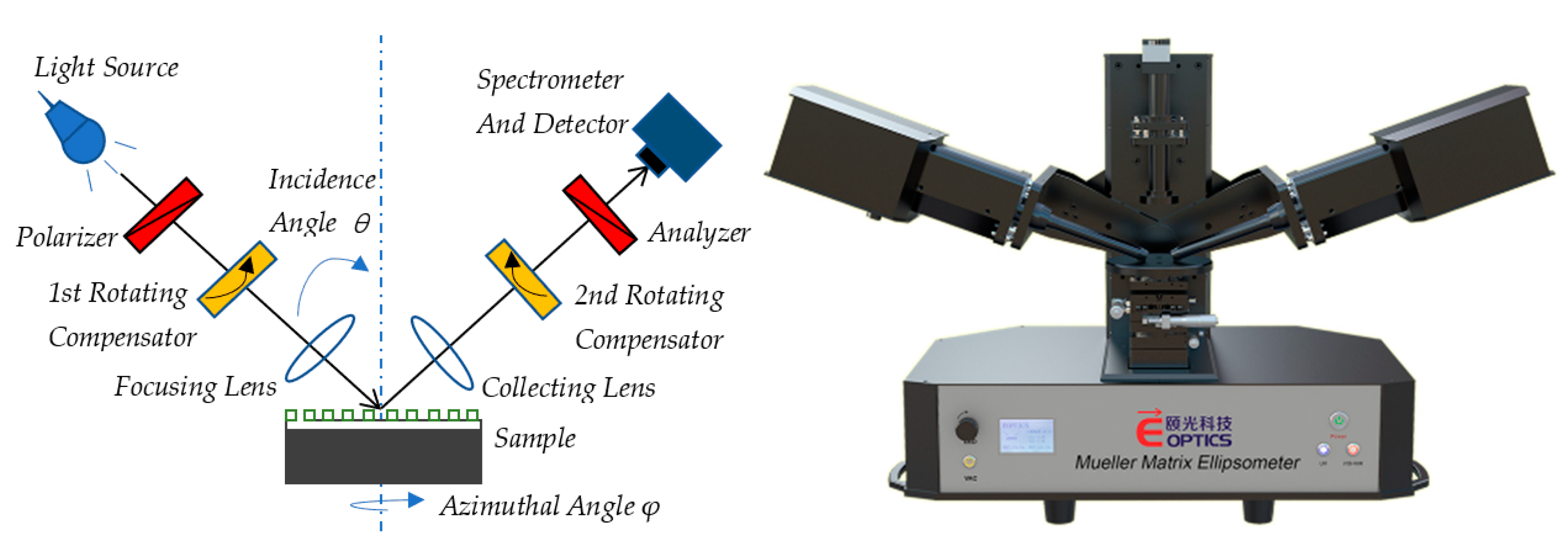
3.1. Experimental Setup

We took spectroscopic scatterometry as an example to demonstrate the capability of the proposed method in identifying and eliminating the measurement configurations with redundant information. The experiments were carried out by a commercial Mueller matrix ellipsometer (ME-L ellipsometer, Wuhan Eoptics Technology Co., China). As schematically shown in Figure 1, the system layout of the dual rotating-compensator ellipsometer in order of light propagation is PC_r1(ω₁)SC_r2(ω₂)A, where P and A stand for the fixed polarizer and analyzer, respectively, C_r1 and C_r2 refer to the 1st and 2nd frequency-coupled rotating compensators, respectively, and S stands for the sample [31,32]. The 1st and 2nd compensators rotate synchronously at ω₁ = 5ω and ω₂ = 3ω, respectively, where ω is the fundamental mechanical frequency. With the light source used in this ellipsometer, the spectral range is from 200 to 1000 nm, covering the spectral range of 300–900 nm used in this work. The beam diameter can be changed from the nominal values of ~3 mm to a value less than 200 μm with the focusing lens. The two arms of the ellipsometer and the sample stage can be rotated to change the incidence and azimuthal angles in experiments. Except for the reflectance and ellipsometric angles of the sample under measurement, the 16 Mueller matrix elements also can be obtained with the dual-rotating compensator setting. An in-house developed MATLAB^® (version R2017a, The MathWorks, Inc., Natick, MA, USA) program for analyzing the measured signatures ran on a workstation equipped with double 2.0 GHz Intel Xeon CPUs. The forward optical model in this program was developed based on rigorous coupled-wave analysis (RCWA) [33,34,35], and the inverse optical scattering problem was solved through the commonly used Levenberg-Marquardt (LM) algorithm [36].

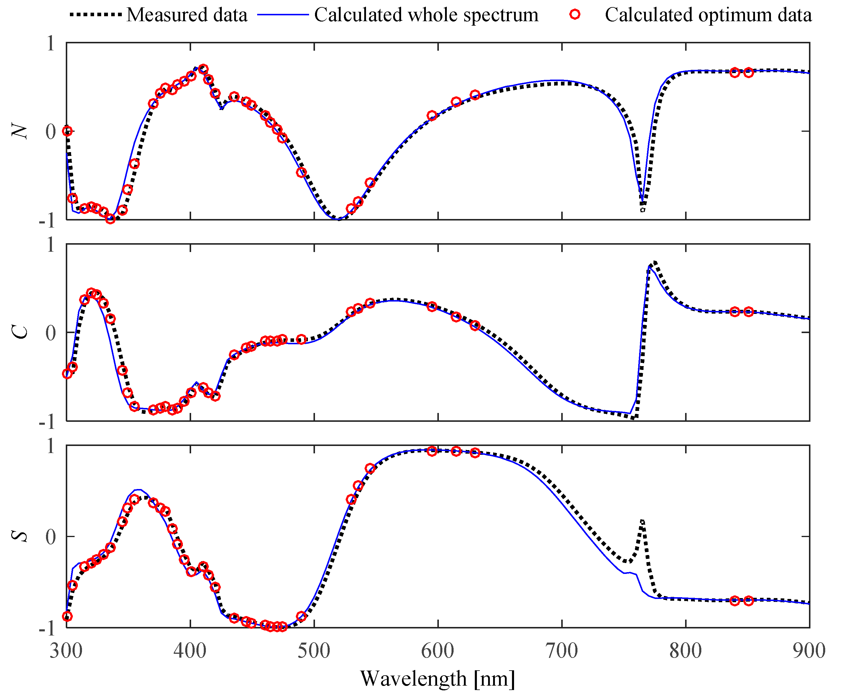
3.2. Experimental Results on 2D Grating

The first investigated sample was a 2D Si grating whose SEM cross-section image is shown in Figure 2. The optical properties of Si were taken from Reference [37]. As depicted in Figure 2, the cross section of the Si grating could be characterized by a symmetrical trapezoidal model with top width (W), grating height (H), sidewall angle (SWA), and period (P), whose dimensions obtained from Figure 2 were W = 350 nm, H = 472 nm, SWA = 87.63°, and P = 800 nm.

In this case, the profile parameters under study were W, H, and SWA, while the grating period P was fixed at its nominal dimension, namely, m = 3. The measured signature contained 15 Mueller matrix elements normalized to the first element, namely, l = 15. As mentioned above, the measurement configuration a = [φ, θ, λ] was defined as a combination of fixed azimuthal angle φ, fixed incident angle θ, but a wide waveband λ for spectroscopic scatterometry. As a simple example to demonstrate our data refinement method, here, the incident and azimuthal angles were fixed at θ = 65° and φ = 30°, the wavelength covered a fixed range of 300~900 nm with a step of 5 nm. We assumed that the dimensions of the three profile parameters under investigation had a deviation of about 1% from their nominal values. The differences of the 15 Mueller matrix elements between the actual and nominal profiles were calculated by our forward RCWA model under each wavelength point according to Equation (5). After considering all the 15 Mueller matrix elements and the wavelengths used, the enanalysis and eigen-analysis procedures described above were performed on the differences. According to Equations (6)–(9), the wavelength points with redundant information were identified and eliminated from the set of measured signatures in a repetitive manner. Since the investigated sample shown in Figure 2 is a simple structure, and the model output Mueller matrix had 15 elements, we achieved the 3 × 15 optimized data sets by traversing the three profile parameters and the 15 Mueller matrix elements. Through merging the same wavelengths into one for the 3 × 15 optimized data sets, the remaining unions S_opt, containing 19 points, were obtained and shown by the black circles in Figure 3, which are supposed to contain enough information needed for the profile reconstruction of the 2D Si grating.

To examine the validity of the remaining information, regression analysis was conducted to reconstruct the three profile parameters from the full spectral range of 300–900 nm, the optimal spectrum containing 19 points, and the spectrum of 19 random points. The non-linear LM algorithm was applied to fit the measured 15 Mueller matrix elements with the modeled ones, which converged very quickly to a minimum when a suitable initial condition was chosen. During the fitting procedure, the root-mean-squared error (RMSE) was used to quantify the goodness of fit, which summed over all the measurement wavelengths the differences between the measured data and model-generated data. The lower the RMSE value, the better the fit or agreement between the measured and model-generated data. Figure 3 presents the fitting result of the model-calculated best-fit Mueller matrix elements (black circles) and the measured spectrum including (red lines) 19 optimal points.

Table 1. Comparison of fitting results of the 2D grating extracted from different spectrum and SEM measurements.

Measuring Mode	Dimensions (nm/°)			RMSE	Time (s)
	W /nm	H /nm	SWA /°
SEM	350.3 ± 4.74	472.1 ± 4.87	87.63 ± 0.611	—	—
Full spectrum	347.3 ± 0.17	468.9 ± 0.20	86.89 ± 0.019	9.44	548
Optimal (19)	347.4 ± 0.15	476.9 ± 0.12	87.27 ± 0.008	8.27	143
Random (19)	345.2 ± 0.74	486.4 ± 0.86	86.31 ± 0.103	13.59	225

shows the extracted profile parameter values for the fits and the SEM-measured values. The uncertainties associated with the SEM-measured values were estimated by manually measuring the SEM micrographs. The uncertainties appended to the scatterometry-determined values were estimated from 30 repeated measurements. All uncertainties correspond to a 95% confidence level. As shown in Table 1, the parameters W, H, and SWA of the 2D grating, extracted by fitting the optimized spectrum, approximately agree with the ones obtained by using the full spectrum, while the former method is over three times faster than the later one; the time spent between the optimal and random measuring modes is slightly different, and the reason may be that the former iterations are a little smaller than the latter during the profile reconstruction procedure as that latter has more sufficient information. Figure 3 shows that the model-calculated 15 Mueller matrix elements match well with the measured spectrum. The experiments performed on the 2D Si grating provide preliminary evidence that the advantages of the proposed method are in speeding up the reconstruction procedure and effectively improving the precision of the extracted parameters.

3.3. Experimental Results on 3D Grating

The second sample was a photoresistive grating consisting of a cylinder array deposited on silicon with a bottom anti-reflective coating (BARC), which is a 3D grating whose SEM cross-section image is shown in Figure 4. The 3D grating of the cylinder array was chosen for this study due to the high computation effort of its forward optical model. As depicted in Figure 4, the cross section of the 3D grating is characterized by a model with cylinder diameter (D) and height (H₁), BARC height (H₂), and periods of arrays in two directions (P_x and P_y). The dimensions obtained from Figure 4 are D = 226.7 nm, H₁ = 355.1 nm, H₂ = 104.3 nm, and P_x = P_y = 835 nm. In our experiments, optical properties of the photoresist were modelled by a two-term Forouhi–Bloomer model [38], whose eight undetermined parameters were determined by measuring a photoresist film deposited on the silicon substrate using the above ellipsometer and were A₁ = 0.006029, A₂ = 0.020598, B₁ = 14.195303 eV, B₂ = 14.196431 eV, C₁ = 50.523937 eV², C₂ = = 50.537878 eV², n (∞) = 1.436087, and E_g = 4.774050 eV. Similarly, optical properties of the BARC were modelled using the Tauc–Lorentz model [39], whose five undetermined model parameters were obtained as ε₁ (∞) = 1.42680, E_g = 3.45971 eV, A = 21.14955, E₀ = 9.94921, C = 0.98767. For more details about physical meanings of the above parameters, one can consult References [38,39], which are omitted here for brevity.

Here, the investigated profile parameters of the 3D grating included the D, the H₁, and the H₂, namely, m = 3, while the two grating periods were fixed at their nominal dimensions. In contrast to the experiment settings above, the incidence and azimuthal angle were fixed at θ = 65° and φ = 0°, and the terms of N, C, and S parameters versus wavelength were used as measured signatures, which were derived from ellipsometric Psi (Ψ) and Delta (Δ) and taken as N = cos (2Ψ), C = sin (2Ψ) cos (Δ), and S = sin (2Ψ) sin (Δ). Considering that the investigated 3D sample deviated largely from its nominal values, its forward model was highly complex and nonlinear, and the model output was N, C, and S, namely, l = 3, we assumed that the dimensions of the three profile parameters changed k = 6 times to ensure that the optimization procedure was stable, and the deviations were about ±1%, ±5%, or ±10% from their nominal dimensions, respectively. According to our proposed method, 3 × 3 × 6 optimized data sets remained, then, the union S_opt of the remaining data sets, consisting of the 36 wavelength points shown in Figure 5, were achieved for the inverse problem solution.

In the same way, the regression analysis was performed to extract the three unknown profile parameters, and the non-linear LM algorithm was also applied to fit the measured signatures with the modeled ones. The extracted profile parameter values for the fits and the SEM-measured values are shown in

Table 2. Comparison of fitting results of the 3D photoresist grating extracted from different spectrum and SEM measurements.

Measuring Mode	Dimensions (nm)			RMSE	Time (hour)
	D /nm	H1 /nm	H2 /nm
SEM	226.7 ± 28.32	355.1 ± 2.05	104.3 ± 1.30	—	—
Full spectrum	249.8 ± 2.56	344.3 ± 1.44	107.6 ± 0.62	28.77	14
Optimal (36)	250.4 ± 2.21	343.9 ± 1.03	106.4 ± 0.51	17.45	4.5
Random (36)	262.4 ± 2.38	338.7 ± 2.42	108.1 ± 0.89	26.50	6

. The uncertainties appended to the SEM-measured and scatterometry-measured values in Table 2 were estimated in a similar manner to those in Table 1. Figure 5 presents the fitting result of the model-calculated best-fit N, C, and S parameters and the measured spectrum (black dots) containing whole range (blue lines) and only 36 optimal points (red circles), respectively.

From Table 2, the three average values of the 3D grating dimensions extracted using 36 optimal points are very close to the values obtained using the full range spectrum, but the extracted parameter D has about a 25 nm deviation from the SEM-measured value, which is probably caused by the obvious non-uniformity of the grating surface depicted in Figure 4, and the SEM-measured values include estimation errors in manually measuring the SEM micrographs. Table 2 also shows that the proposed method results in the lowest value of RMSE, the highest measurement precision, and the least time cost. It is observed from Figure 5 that the best-fit N, C, and S parameters using the optimized spectrum are in better agreement with the measured signatures compared to those of the full range. Consequently, we may conclude that the proposed dependence-analysis-based data-refinement method can be applied to determine several optimal measurement points without any loss in the accuracies for profile reconstruction in optical scatterometry.

4. Conclusions

In summary, we proposed a method to identify and eliminate the measurement configurations with redundant information based on dependence analysis in optical scatterometry. By assuming that the dimensions of profile parameters under investigation have some deviation from their nominal values, the differences between the actual and nominal dimensions were calculated by the forward optical model under each measurement point. A formulation was derived to identify the measurement configurations with redundant information through performance of a dependence analysis followed by an eigen-analysis. By eliminating redundant information from the measured data in a repetitive manner, a few optimal points remained and were used for the reconstruction process.

Experiments performed on a 2D Si grating and a 3D photoresist grating revealed that the reconstructed grating profiles from the optimally selected subset of measurement wavelengths according to the proposed method have a higher accuracy than those from the randomly selected counterparts with a higher efficiency than the analysis making use of the whole spectrum. This suggests that the proposed dependence-analysis-based data-refinement method can be a powerful tool to enhance the reconstruction speed of nanostructure metrology using scatterometry without sacrificing the accuracies, especially for the nanostructures whose forward model is very complex and time-consuming.

References

1. Fang, F.Z.; Zhang, X.D.; Gao, W.; Guo, Y.B.; Byrne, G.; Hansen, H.N. Nanomanufacturing – Perspective and applications. CIRP Ann. Manuf. Technol. 2017, 66, 683–705. [Google Scholar] [CrossRef]
2. Bundary, B.; Solecky, E.; Vaid, A.; Bello, A.F.; Dai, X. Metrology capabilities and needs for 7nm and 5nm logic nodes. Proc. SPIE 2017, 10145, 101450G. [Google Scholar]
3. Sunkoju, S.; Schujman, S.; Dixit, D.; Diebold, A.; Li, J.; Collins, R.; Haldar, P. Spectroscopic ellipsometry studies of 3-stage deposition of CuIn1 _ XGaXSe2 on Mo-coated glass and stainless steel substrates. Thin Solid Films 2016, 606, 113–119. [Google Scholar] [CrossRef]
4. Lereu, A.L.; Passian, A.; Farahi, R.H.; Abel-Tiberini, L.; Tetard, L.; Thundat, T. Spectroscopy and imaging of arrays of nanorods toward nanopolarimetry. Nanotechnology 2012, 23, 045701. [Google Scholar] [CrossRef]
5. Hansen, H.N.; Carneiro, K.; Haitjema, H.; Chiffre, L.D. Dimensional micro and nano metrology. CIRP Ann. Manuf. Technol. 2006, 55, 721–743. [Google Scholar] [CrossRef]
6. Huang, H.T.; Kong, W.; Terry, F.L., Jr. Normal-incidence spectroscopic ellipsometry for critical dimension monitoring. Appl. Phys. Lett. 2001, 78, 3983–3985. [Google Scholar] [CrossRef] [Green Version]
7. Matthias, W.; Johannes, E.; Jürgen, P.; Max, S.; Alexander, D.; Bernd, B. Metrology of nanoscale grating structures by UV scatterometry. Opt. Express 2017, 25, 2460–2468. [Google Scholar]
8. Faruk, M.G.; Zangooie, S.; Angyal, M.; Watts, D.K.; Sendelbach, M.; Economikos, L.; Herrera, P.; Wilkins, R. Enabling scatterometry as an in-line measurement technique for 32nm BEOL application. IEEE Trans. Semicond. Manuf. 2011, 24, 499–512. [Google Scholar] [CrossRef]
9. Kim, Y.N.; Paek, J.S.; Rabello, S.; Lee, S.; Hu, J.; Liu, Z.; Hao, Y.; McGahan, W. Device based in-chip critical dimension and overlay metrology. Opt. Express 2009, 17, 21336–21343. [Google Scholar] [CrossRef] [PubMed]
10. Patrick, H.J.; Gemer, T.A.; Ding, Y.F.; Ro, H.W.; Richter, L.J.; Soles, C.L. Scatterometry for in situ measurement of pattern flow in nanoimprinted polymers. Appl. Phys. Lett. 2008, 93, 233105. [Google Scholar] [CrossRef]
11. Paz, V.F.; Peterhänsel, S.; Frenner, K.; Osten, W. Solving the inverse grating problem by white light interference Fourier scatterometry. Light Sci. Appl. 2012, 1, e36. [Google Scholar]
12. Chen, X.; Liu, S.; Zhang, C.; Jiang, H. Measurement configuration optimization for accurate grating reconstruction by Mueller matrix polarimetry. J. Micro/Nanolith. MEMS MOEMS 2013, 12, 033013. [Google Scholar] [CrossRef]
13. Zhu, J.; Liu, S.; Zhang, C.; Chen, X.; Dong, Z. Identification and reconstruction of diffraction structures in optical scatterometry using support vector machine method. J. Micro/Nanolith. MEMS MOEMS 2013, 12, 013004. [Google Scholar] [CrossRef]
14. Zhang, C.; Liu, S.; Shi, T.; Tang, Z. Fitting-determined formulation of effective medium approximation for 3D trench structures in model-based infrared reflectrometry. J. Opt. Soc. Am. A 2011, 28, 263–271. [Google Scholar] [CrossRef] [PubMed] [Green Version]
15. Zallat, J.; Aïnouz, S.; Stoll, M.P. Optimal configurations for imaging polarimeters: Impact of image noise and systematic errors. J. Opt. A Pure Appl. Opt. 2006, 8, 807–814. [Google Scholar] [CrossRef]
16. Zaharov, V.V.; Farahi, R.H.; Snyder, P.J.; Davison, B.H.; Passian, A. Karhunen-Loève treatment to remove noise and facilitate data analysis in sensing, spectroscopy and other applications. Analyst 2014, 139, 5927–5935. [Google Scholar] [CrossRef] [PubMed]
17. Mu, T.; Chen, Z.; Zhang, C.; Liang, R. Optimal configurations of full-Stokes polarimeter with immunity to both Poisson and Gaussian noise. J. Opt. 2016, 18, 055702. [Google Scholar] [CrossRef]
18. Logofǎtu, P.C. Sensitivity analysis of grating parameter estimation. Appl. Opt. 2002, 41, 7179–7186. [Google Scholar] [CrossRef]
19. Ku, Y.; Wang, S.; Shyu, D.; Smith, N. Scatterometry-based metrology with feature region signature matching. Opt. Express 2006, 14, 8482–8491. [Google Scholar] [CrossRef]
20. Vagos, P.; Hu, J.; Liu, Z.; Rabello, S. Uncertainty and sensitivity analysis and its applications in OCD measurement. Proc. SPIE 2009, 7272, 72721N. [Google Scholar]
21. Dong, Z.; Liu, S.; Chen, X.; Shi, Y.; Zhang, C.; Jiang, H. Optimization of measurement configuration in optical scatterometry for one-dimensional nanostructures based on local sensitivity analysis. J Infrared Millim Waves 2016, 1, 116–122. [Google Scholar]
22. Dong, Z.; Liu, S.; Chen, X.; Zhang, C. Determination of an optimal measurement configuration in optical scatterometry using global sensitivity analysis. Thin Solid Films 2014, 562, 16–23. [Google Scholar] [CrossRef]
23. Twomey, S. Indirect measurements of atmospheric temperature profiles from satellites: II. Mathematical aspects of the inverse problem. Mon Weather Rev 1966, 96, 363–366. [Google Scholar] [CrossRef]
24. Twomey, S.; Howell, H.B. Some Aspects of the Optical Estimation of Microstructure in Fog and Cloud. Appl. Opt. 1967, 6, 2125–2131. [Google Scholar] [CrossRef] [PubMed]
25. Twomey, S. Information content in remote sensing. Appl. Opt. 1973, 13, 942–945. [Google Scholar] [CrossRef] [PubMed]
26. Al-Assaad, R.A. Scatterometry for Semiconductor Sub-Micrometer and Nanometer Critical Dimension Metrology. Ph. D. Thesis, University of Texas, Austin, TX, USA, 2006. [Google Scholar]
27. Kirsch, A. Uniqueness theorems in inverse scattering theory for periodic structures. Inverse Probl. 1994, 10, 145–152. [Google Scholar] [CrossRef]
28. Kirsch, A. An Introduction to the Mathematical Theory of Inverse Problems, 2nd ed.; Springer: New York, NY, USA, 2011. [Google Scholar]
29. Yang, J.; Zhang, B. Uniqueness results in the inverse scattering problem for periodic structures. Math. Method. Appl. Sci. 2012, 35, 828–838. [Google Scholar] [CrossRef]
30. Chen, X.; Liu, S.; Gu, H.; Zhang, C. Formulation of error propagation and estimation in grating reconstruction by a dual-rotating compensator Mueller matrix polarimeter. Thin Solid Films 2014, 571, 653–659. [Google Scholar] [CrossRef]
31. Collins, R.W.; Koh, J. Dual rotating-compensator multichannel ellipsometer: Instrument design for real-time Mueller matrix spectroscopy of surfaces and films. J. Opt. Soc. Am. A 1999, 16, 1997–2006. [Google Scholar] [CrossRef]
32. Liu, S.; Chen, X.; Zhang, C. Development of a broadband Mueller matrix ellipsometer as a powerful tool for nanostructure metrology. Thin Solid Films 2015, 584, 176–185. [Google Scholar] [CrossRef]
33. Moharam, M.G.; Pommet, D.A.; Grann, E.B.; Gaylord, T.K. Stable implementation of the rigorous coupled-wave analysis for surface-relief gratings: Enhanced transmittance matrix approach. J. Opt. Soc. Am. A 1995, 12, 1077–1086. [Google Scholar] [CrossRef]
34. Li, L. New Formulation of the Fourier modal method for crossed surface-relief gratings. J. Opt. Soc. Am. A 1997, 14, 2758–2767. [Google Scholar] [CrossRef]
35. Liu, S.; Ma, Y.; Chen, X.; Zhang, C. Estimation of the convergence order of rigorous coupled-wave analysis for binary gratings in optical critical dimension metrology. Opt. Eng. 2012, 51, 081504. [Google Scholar] [CrossRef]
36. Press, W.H.; Teukolsky, S.A.; Vetterling, W.T.; Flannery, B.P. Numerical Recipies: The Art of Scientific Computing, 3rd ed.; Cambridge University Press: Cambridge, UK, 2007; Chapter 15. [Google Scholar]
37. Herzinger, C.M.; Johs, B.; Mcgahan, W.A.; Woollam, J.A.; Paulson, W. Ellipsometric determination of optical constants for silicon and thermally grown silicon dioxide via a multi-sample, multi-wavelength, multi-angle investigation. J. Appl. Phys. 1998, 83, 3323–3336. [Google Scholar] [CrossRef]
38. Forouhi, A.R.; Bloomer, I. Optical properties of crystalline semiconductors and dielectrics. Phys. Rev. B 1988, 38, 1865–1874. [Google Scholar] [CrossRef] [PubMed]
39. Jellison, G.E., Jr.; Modine, F.A. Parameterization of the optical functions of amorphous materials in the interband region. Appl. Phys. Lett. 1996, 69, 371–373. [Google Scholar] [CrossRef]
Figure 1. Principle and instrument of the dual rotating-compensator Mueller matrix ellipsometer.
Applsci 09 04091 g001
Figure 2. Scanning electron microscopy (SEM) cross-section image of the investigated 2D Si grating sample.
Applsci 09 04091 g002
Figure 3. Fitting results of the calculated and the ellipsometer-measured Mueller matrix elements with the incidence and azimuthal angles fixed at θ = 65° and φ = 30°, respectively.
Applsci 09 04091 g003
Figure 4. SEM cross-section image of the investigated 3D grating sample.
Applsci 09 04091 g004
Figure 5. Fitting results of the calculated and the ellipsometer-measured N, C, and S parameters at the incidence angle θ = 65° and azimuthal angle φ = 0°.
Applsci 09 04091 g005