MFCSNet: Multi-Scale Deep Features Fusion and Cost-Sensitive Loss Function Based Segmentation Network for Remote Sensing Images

Abstract

Semantic segmentation of remote sensing images is an important technique for spatial analysis and geocomputation. It has important applications in the fields of military reconnaissance, urban planning, resource utilization and environmental monitoring. In order to accurately perform semantic segmentation of remote sensing images, we proposed a novel multi-scale deep features fusion and cost-sensitive loss function based segmentation network, named MFCSNet. To acquire the information of different levels in remote sensing images, we design a multi-scale feature encoding and decoding structure, which can fuse the low-level and high-level semantic information. Then a max-pooling indices up-sampling structure is designed to improve the recognition rate of the object edge and location information in the remote sensing image. In addition, the cost-sensitive loss function is designed to improve the classification accuracy of objects with fewer samples. The penalty coefficient of misclassification is designed to improve the robustness of the network model, and the batch normalization layer is also added to make the network converge faster. The experimental results show that the classification performance of MFCSNet outperforms U-Net and SegNet in classification accuracy, object details and prediction consistency.

1. Introduction

Remote sensing images are important data for spatial information processing. Automatic analysis of feature information in images has an important application significance [1,2,3,4,5,6]. Remote sensing image fully exploits geographic information, which is of great significance in the fields of forestry monitoring [2], water system monitoring [3] and geological exploration [4]. Remote sensing technology analysis of ground objects and their changes with time and space have great application significance in the fields of military reconnaissance, economic construction, meteorological forecasting [5,6,7,8] and earthquake disaster early warning [9], which are related to the national economy and people’s livelihood. A large amount of urban geographic information contained in remote sensing images, which can be used in many fields, such as digital cities, intelligent transportation, navigation maps, and urban planning [10,11]. Therefore, automatic analysis of remote sensing images has become an important research topic for geospatial information detection.

Remote sensing image contains a wealth of feature information. Rich geospatial information can be obtained through automatic classification methods to serve all aspects of human’s life. The multi-objective classification of remote sensing images is to assign a label to each pixel in the image. It divides the image into different semantic regions. The researchers have carried out many explorations.

In the 1980s, the statistical analysis of the features of remote sensing images is the mainstream method, which required different feature extraction methods for different tasks [12]. The development of digital image processing has promoted the advancement of image analysis, and remote sensing image classification can be realized based on artificial features. Commonly features include color histogram [13], direction gradient histogram [14] and scale-invariant feature transform [15], which contain a large amount of information. The artificial feature-based method can deal with some basic remote sensing image classification problems, but for more complex remote sensing images, it cannot achieve the desired performance.

In recent years, machine learning is developing rapidly, which leads to many remote sensing image classification and semantic segmentation algorithms based on machine learning methods are proposed. For example, Wang et al. [16] jointly used low-rank representation (LRR), spectral-spatial graph regularization and subspace learning to classify the objects in hyperspectral images, and proposed a self-supervised low-rank representation framework. Ma et al. [17] used classification and regression tree (CART) to classify remote sensing images, which achieved the accurate classification of different land objects in remote sensing image. However, its performance still needs to be improved. Réjichi S et al. [18] used principal component analysis to preserve the main information of the image and reduce the feature’s dimension. This method can obtain the invariant features in the classification task, which improves the efficiency of classification. Zhao et al. [19] used K-means to segment remote sensing image. In this method, the initial class number and centers are determined by the probability density function of the first principal component. The machine learning-based remote sensing image classification methods have achieved good results and strong stability. With the increasing demand for remote sensing image interpretation, the goals are becoming more complex and diverse. The algorithms based on feature engineering and shallow learning model are not suitable to solve the complex multi-class classification of remote sensing image.

Deep learning has been widely used in many fields. This kind of method autonomously learns data features through massive training data, which greatly accelerates the development of image recognition. In 2006, Hinton used the back propagation algorithm to train the deep confidence network [20], which greatly improved the recognition performance. Common image classification networks include LeNet [21], AlexNet [22], ResNet [23], etc. Later, the proposed Regions with Convolutional Neural Networks (RCNN) [24] opened up a research boom using the deep learning method for object detection. The object detection network can not only identify the object, but also identify the position of the object in the image. Object detection networks include Faster RCNN [25], SSD [26], YOLO [27], etc.

With the development of image classification and object detection algorithms, scholars have proposed networks for pixel-level classification of images, which can assign a label to each pixel in the image. For example, Shelhamer E et al. [28] proposed a fully convolutional network (FCN) for semantic segmentation. This network can achieve end-to-end pixel-level classification of images, which greatly improves the efficiency of remote sensing image object classification. In 2015, Vijay et al. 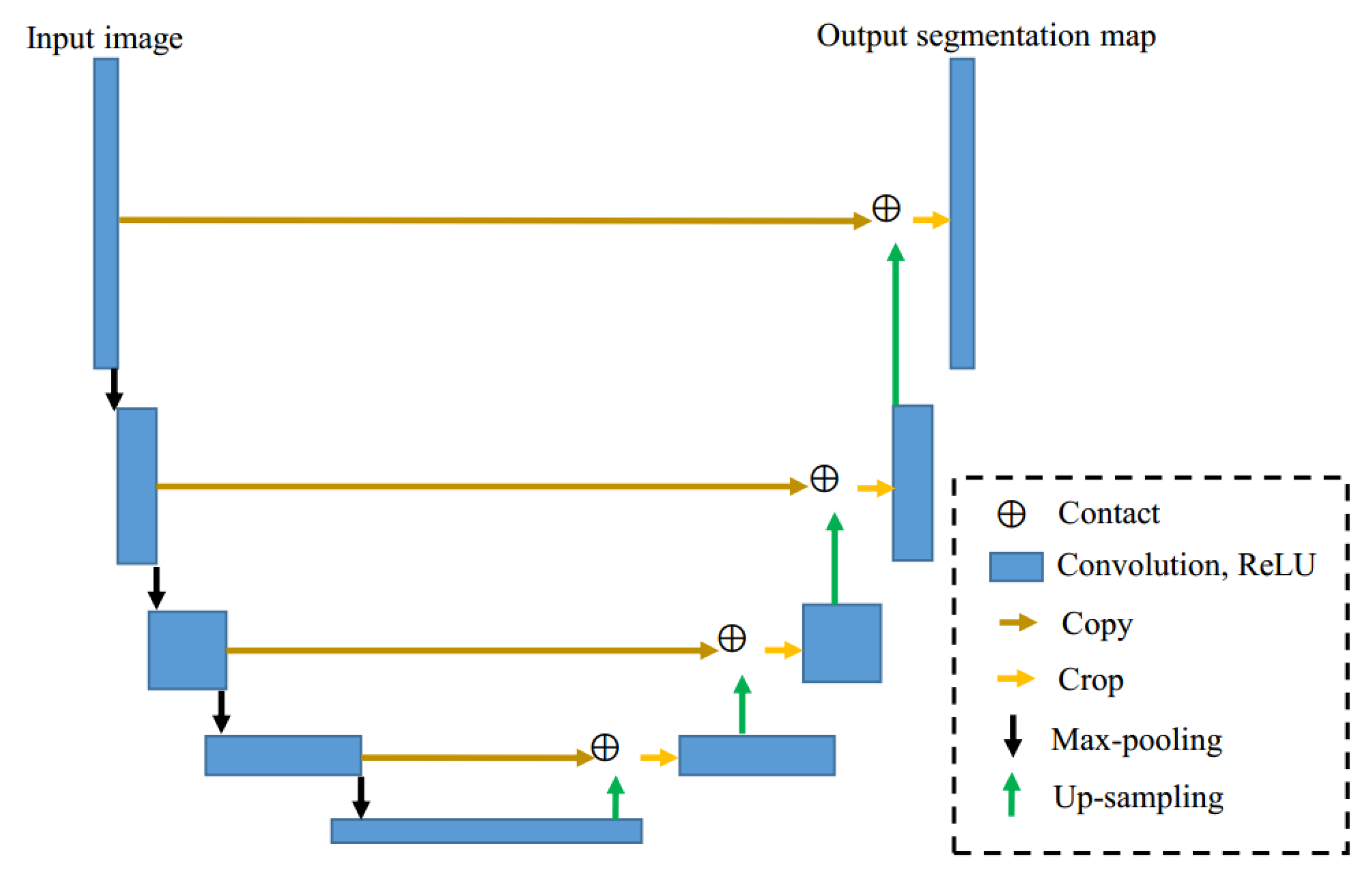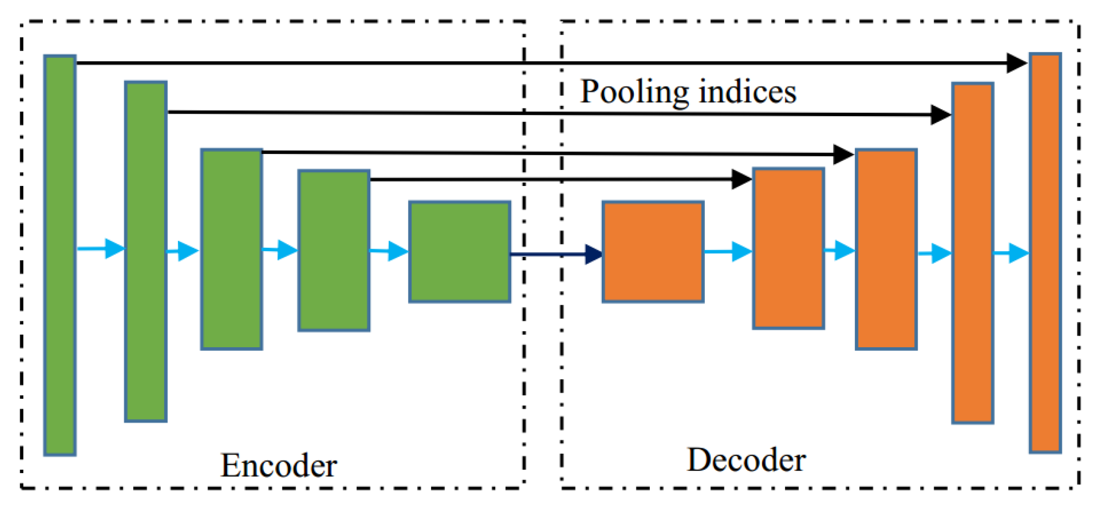[29] proposed a semantic segmentation network, named SegNet. It consists of an encoding structure and a decoding structure, which preserved the details of the image by saving the position index in the pooling process. At the same year, U-Net [30] is proposed by for semantic segmentation of the image, which makes full use of the low-level semantic information of the image in the up-sampling process. It can achieve good results in image segmentation with fewer samples. Besides, some effective networks (e.g., References [31,32,33,34]) are proposed for remote sensing image. For example, He et al. [35] use deep confidence network to analyze remote sensing data. The network training speed is fast, and it is not easy to fall into local optimum. Although it has achieved good classification performance, the accuracy of object recognition still needs to be improved.

To achieve effective semantic segmentation performance of remote sensing image, we design multi-scale feature encoding structure and max-pooling indices decoding structure. In addition, we propose cost-sensitive loss function, and introduce batch normalization layer to accelerate network convergence process.

The main contributions of this paper are as follows:

1. This paper presents a novel multi-scale deep features fusion and cost-sensitive loss function based semantic segmentation network for remote sensing images, named MFCSNet. Combining the advantages of U-Net and SegNet, a multi-scale feature encoding structure and a max-pooling indices decoding structure is designed. The MFCSNet can fully extract the features of the remote sensing image. This network can integrate the low-level semantic information and high-level semantic information. The max-pooling indices up-sampling method retains the details, such as the object edge, which can effectively improve the network classification effect.

2. In order to solve the problem of low classification accuracy of objects with few pixels in complex remote sensing images. This paper designs a cost-sensitive loss function. The MFCSNet obtains a more robust network model by raising the penalty coefficient for the misclassified samples. Besides, the batch normalization layer and standardizing the distribution of neural network output are used to improve the network convergence speed, which can improve the classification performance of the network.

2. Related Work

After the FCN was proposed for semantic segmentation, the researchers conducted many researches and improvements on its structural design and theory. In the field of image multi-objective classification, many deep learning networks have been proposed. U-Net and SegNet are two state-of-the-art network models. The U-Net structure is relatively simple and clear. It has a few network parameters, high training and testing efficiency, and low dependence on the number of samples. However, the details extraction and processing of the object edge still need to be improved. For SegNet, it retains more object location and neighborhood information. However, the extracted features of SegNet are insufficient and incomprehensive caused by the sample feature extraction structure. Considering the advantages and disadvantages of U-Net and SegNet, we can propose the improved network for remote sensing image semantic segmentation. Thus, this section introduces these two related networks as the basic methods.

2.1. U-Net Network

U-Net consists of two parts, as shown in Figure 1. The feature extraction part is on the left, and the up-sampled part is on the right. The feature extraction part is composed of convolution layers and pooling layers of different scales, so that different scales features of the image can be extracted. The up-sampling portion fuses the current sampling feature and the feature image of the corresponding feature extraction portion at each time. This can merge the low-level features and high-level features, and the low-level features help provide edge information which can solve the object pixels location problem.

As shown in Figure 1, the feature extraction part is used to extract multi-scale features of the image. Each down-sampling stage includes two convolution layers with a convolution kernel size of 3 × 3 and a pooling layer with a kernel size of 2 × 2. The active function is ReLU. After down-sampling, the image size is reduced by half, and the number of channels is doubled. In the up-sampling section, each up-sampling stage consists of two convolution layers with a convolution kernel size of 3 × 3 and a deconvolution layer with a kernel size of 2 × 2. After each up-sampling, the channel of the image is reduced by half, and the size of the image is doubled. In the output layer of the network, the feature space-to-output mapping is convoluted by a convolution layer with a convolution kernel size of 1 × 1. Finally, the class of each pixel is predicted.

2.2. SegNet Network

SegNet network is an end-to-end convolution neural network to achieve pixel-level classification. It consists of two parts, i.e., the encoding structure and the decoding structure, as shown in Figure 2. The encoding structure continuously extracts features of various scales of the image through the convolution layer and the pooling layer. The pooling process of SegNet is different from the traditional pooling process. In addition, SegNet uses the encoder to save the location information corresponding to the maximum value in the original feature map. The location information will be used during up-sampling. The feature map of the decoding structure is up-sampled, and the image is gradually restored to the original image size in combination with the encoded feature map to achieve pixel-level classification.

The SegNet encoding process consists of five phases. The first two phases consist of two 3 × 3 convolution layers and a 2 × 2 pooling layer. The next three down-sampling stages include three 3 × 3 convolution layers and a 2 × 2 pooling layer with ReLU. In the max-pooling process, the encoder is used to record the position index of the maximum value. The decoding process is symmetric with the encoding process, and it consists of five phases. The first three phases consist of a 2 × 2 up-sampling layer and three 3 × 3 convolution layers. The last two phases consist of a 2 × 2 up-sampling layer and two 3 × 3 convolution layers. At the end of the network, the classification prediction results for each pixel are output by the softmax function. By introducing fully convolution layers, SegNet greatly reduces network parameters. It also improves the execution efficiency of the entire network, and realizes end-to-end pixel-level classification. The SegNet network has achieved good results in the semantic segmentation, but it still needs to be further improved in the feature extraction structure.

3. Proposed Method

SegNet network retains the location information of the object through the max-pooling indices. The U-Net network realizes the combination of the low-level image features and the high-level image features through the multi-level jump structure, which can extract fuller features and reduce the dependence on the number of samples. Thus, we improve U-Net and SegNet networks to propose a new multi-scale deep features fusion and cost-sensitive loss function based multi-object classification network for remote sensing images, named MFCSNet.

As shown in Figure 3, the improved network in this paper consists of the encoding part (on the left side) and the decoding part (on the right side). The multi-scale feature encoding structure is used to extract each scale features of the input image continuously. This process includes convolution layers and pooling layers. Then the up-sampling is continuously performed by the decoding structure. To accurately retain the location information of the object features, the up-sampling is achieved by the max-pooling indices structure.

In order to make full use of the shallow features, such as texture and edge of the image, the corresponding feature map in the feature coding structure is continuously combined during up-sampling. Thereby, the overall classification performance of the network can be improved. To improve the classification accuracy for the objects with a small number of samples, we propose a cost-sensitive loss function, which improves the classification performance of the network. The network details of each part will be discussed in the following.

3.1. Multi-Scale Feature Encoding Structure

In order to extract the essential features of different objects in remote sensing images, we design a feature encoding structure consisting of thirteen convolution layers and five pooling layers, as shown in Figure 3. The convolution kernels of the convolution layers conv1_1, conv1_2 to conv5_3 have the kernel size of 3 × 3. The number of convolution operation channels is shown in Figure 3. In the first convolution layer, the input color image is convoluted by the convolution kernel, whose number of channels is 64 and kernel size is 3 × 3. The shape of the output feature map is 64 × 256 × 256. After five stages of convolution and pooling operations, features of different scales can be obtained.

The activation function converts the linear mapping of the convolution layer into a non-linear mapping. The activation function used in this paper is ReLU. ReLU has the characteristics of simple calculation and stable gradient value, which can effectively solve the problem of too small gradient or gradient explosion.

There are five pooling layers in the encoding structure, such as MaxPool1, MaxPool2 to MaxPool5. The pooling layer adopts the max-pooling mode, and the size of the pooling kernel is 2 × 2. During the pooling process, the maximum index position of each pooling operation is recorded and released during the decoding process, so that the location information of the object can be retained. The pooling layer can compress the feature map, and reduce the number of network parameters, the calculation time and space complexity. Feature compression can extract key information in the image, which can improve classification performance. During the convolution and pooling operations, if the size of the feature map is halved, the number of channels of the convolution kernel is doubled to obtain a richer feature of the image.

3.2. Max-Pooling Indices Decoding Structure

After feature encoding, image features of different scales are obtained. The sizes of these feature maps are 1/2, 1/4, 1/8, 1/16, and 1/32 of the original image sizes, as shown in Figure 3. By performing an up-sampling operation on the feature map, the feature map can be gradually restored to the original image size to obtain the class attribution of each pixel.

The size of objects in remote sensing images is generally small. Thus, the sharpness of their outlines is easily affected by factors, e.g., illumination and weather, which brings difficulties to the object classification task. To solve this problem, we fully consider the details of the object area and its location information. We design the decoding network through the max-pooling indices in the up-sampling process. After the up-sampling is completed, the result is merged with the feature map in the encoding process, so that the shallow contour information of the remote sensing image and the deep semantic information are transmitted in the network.

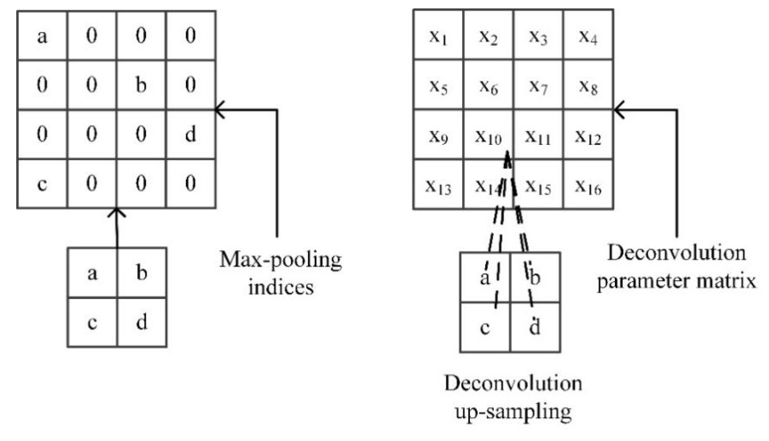
Unlike the method of deconvolution up-sampling. In this paper, the up-sampling method records the max-pooling location during the network encoding process for up-sampling.

As shown in Figure 4, when the max-pooling indices are up-sampled, the feature map is mapped to the up-sampled result according to the maximum coordinate information recorded in the encoding process, and the other non-indexed locations are supplemented with zero, so that the original information can be accurately retained. The location information of the maximum value avoids the loss of information during the up-sampling process. The deconvolution up-sampling method is to deconvolute the feature map by the deconvolution parameter matrix to obtain the up-sampled feature map. It can be seen that the deconvolution calculation process is essentially the inverse of the convolution calculation. After the up-sampling operation is performed using the max-pooling indices, the obtained feature map size is doubled before the up-sampling. Then the feature map contains key feature information of a scale on the image.

Before the convolution in the decoding structure, the up-sampled feature map obtained from the previous stage is connected to the feature map of the corresponding size in the encoding process, such as the structure shown by Concat1, Conact2 to Concat4. By adding a jump structure during the up-sampling process, the low-level features can be reused. The shallow network can acquire information, such as edges and textures of the image. The deep network can learn the semantic information of the image. This structure has a greater receptive field. Such a structure realizes the fusion of the low-level information and the high-level information, so that the network has a richer feature learning ability. In addition, this jumped connection structure does not introduce excessive computational complexity and model complexity, allowing the gradient to propagate efficiently in the network. After the max-pooling indices operation, the convolution operation smooths the abrupt points caused by zero padding.

The multi-objective classification network of remote sensing images designed in this paper stores the max-pooling location during the encoding process, and releases the information in the decoding process. This method can save the key information of the image and accurately record the location information of the object. The semantic information obtained by up-sampling and the contour, texture and spectrum information obtained by the encoding process. These features are fully exploited to improve the network classification ability and the overall performance of the network.

3.3. Batch Normalization Acceleration Layer

The multi-objective classification network of remote sensing images designed in this paper is depth, which can fully learn the features of the image. However, as the network depth increases, the network convergence becomes more and more difficult, and the training speed becomes worse. Therefore, we design a batch normalization (BN) layer in the full convolution neural network. In this way, the input of each layer satisfies the same distribution, and can accelerate the convergence of the network. As the network deepens, the distribution of the activation input values gradually shifts, which causes the network to converge slowly. Through the batch normalization method, the distribution of the input values is transformed into a normal distribution, which the variance is 0, and the mean is 1. It avoids the gradient disappearance and the gradient dispersion problem. The normalized formula is:

$${\widehat{x}}^{(k)}=\frac{x^{(k)}-E[x^{(k)}]}{\sqrt{Var[x^{(k)}]}},$$

(1)

where x represents the input vector of the network, E[x^(k)] represents the mean of the input, and Var[x^(k)] represents variance.

The normalization operation can enhance the flow of backpropagation information and accelerate the convergence of the network. However, such a transformation can also lead to poor expression of the network, which is fatal for networks that need to learn complex features. In order to solve this problem, two adjustment parameters need to be added to each neuron. The inverse transformation of the transformed activation is used to restore the normalized data to a certain extent. The average value μ_B and the variance σ_B² are obtained for the batch as follows:

$${\mu }_B\leftarrow \frac{1}{m}{\displaystyle \sum _{i=1}^m{{\displaystyle x}}_i},$$

(2)

$${\sigma }_B^2\leftarrow \frac{1}{m}{\displaystyle \sum _{i=1}^m{{\displaystyle (x_i-{\mu }_B)}}^2}.$$

(3)

Batch normalization:

$${\widehat{x}}_i\leftarrow \frac{x_i-{\mu }_B}{\sqrt{{\sigma }_B^2+\in }}.$$

(4)

Perform scale and translation transformations:

$$y_i\leftarrow \gamma {\widehat{x}}_i+\beta \equiv B{N}_{\gamma ,\beta (x_i)},$$

(5)

where x represents a mini-batch input value, and B represents the parameters that need to be learned. Then the normalization of the network input during the training process can be completed. After the trained model is obtained, the batch normalization of the test process is to obtain the mean and variance for the entire data set, which is different from the current batch used in the training process. During the training process, it is necessary to record the mean and variance of each batch and perform unbiased estimation as the basis for batch normalization in the testing process.

The network convergence process can be significantly accelerated, followed by the batch normalization. The training time can be reduced. The network can use a large learning rate, and the classification performance of the network is improved to some extent. If the input scales of the layers in the network differ greatly, then the training of the network should be performed using a lower learning rate according to the barrel theory. After introducing the batch normalization layer, data can be normalized to the same scale, which allows for a larger learning rate. This makes the network less sensitive to the learning rate, and makes network parameters optimization easier. This method is convenient to obtain a better remote sensing image classification network.

3.4. Cost-Sensitive Loss Function

For the neural network, the smaller the loss function, the stronger the performance of the network model. Generally, loss functions are square loss function, exponential loss function and cross-entropy loss function. The neural network designed in this paper uses the cross-entropy loss function and improves it for multi-objective classification tasks of remote sensing images.

Remote sensing images contain complex objects and unbalanced samples. For example, vegetation types account for a large proportion of remote sensing images, while roads and other objects often occupy only a small number of pixels in remote sensing images. In the process of neural network learning, the class with a small number of samples is prone to under-fitting. In order to solve this problem, we add a cost-sensitive matrix to the loss function. Thus, the network model has a larger penalty when it misclassifies a few sample categories, and it strengthens the attention of this class sample.

For multi-classification, assuming that the total number of samples in the training data set is N, and the number of classes is M. The size of cost-sensitive matrix W is M × M, which can be set to balance the penalty weights for different misclassified samples.

$$W=\left[\begin{array}{cccc}\mathrm{w}(1,1)& \mathrm{w}(1,2)& \dots & \mathrm{w}(1,\mathrm{M})\\ \mathrm{w}(2,1)& \mathrm{w}(2,2)& \dots & \mathrm{w}(2,\mathrm{M})\\ \dots & \dots & \dots & \dots \\ \mathrm{w}(\mathrm{M},1)& \mathrm{w}(\mathrm{M},2)& \dots & \mathrm{w}(\mathrm{M},\mathrm{M})\end{array}\right],$$

(6)

where w(j,k) represents the penalty when the class j is misclassified as the class k. The elements on the diagonal of the matrix W are 0. The values of the cost-sensitive matrix are set according to the number of samples and the confusion matrix in the classification result. By introducing a cost-sensitive matrix to the loss function, the influence of samples imbalance on the performance of the network can be reduced. Then, the classification performance on a smaller number of categories can be improved.

3.5. Network Training and Optimization

The forward propagation algorithm and the back propagation algorithm are two processes for convolution neural network training. The process of forward propagation is the process of getting the corresponding output based on the input. The backpropagation algorithm reversely transmits the error value according to the error between the output value and the true value. Backpropagation algorithm corrects the connection weight between the neurons to obtain the network model with the smallest error.

For a data set containing m samples {(x⁽¹⁾,y⁽¹⁾),…,(x^(m),y^(m))}, O_W,b(x) represents the output value of the sample (x, y) after classified by the network. To perform iterative optimization of the network, define the following cost function:

$$J(W,b;x,y)=\frac{1}{2}{\Vert o_{W,b}(x)-y\Vert }^2.$$

(7)

Considering m samples in the data set, an expression for their overall cost function can be obtained:

$$J(W,b)=\left[\frac{1}{m}{\displaystyle \sum _{i=1}^{m}J(W,b;x^{(i)},y^{(i)})}\right]+\frac{\lambda }{2}{\displaystyle \sum _{l=1}^{n_l-1}{\displaystyle \sum _{i=1}^{s_l}{\displaystyle \sum _{j=1}^{s_{l+1}}{\left(W_{ji}^{(l)}\right)}^2}}}.$$

(8)

In Formula (8), the first term represents the mean square error term, reflecting the deviation between the predicted value and the true value. The second term is a regularization term that prevents overfitting, expressed in terms of the complexity of the hyperparameters.

The backpropagation algorithm uses gradient descent and chain derivation rules to calculate the parameters. It continuously corrects the values of the hyperparameters W and b in the iteration to gradually reduce the error. The backpropagation training method has the following steps: First, the forward propagation algorithm is used to obtain the output values of the network, the activation values and weights of each layer of the network. Then, the error of each output neuron can be calculated. The error calculation formula is as follows:

$${\delta }_i^{(n_l)}=\frac{\partial }{\partial z_i^{(n_l)}}\frac{1}{2}{\Vert y-o_{W,b}(x)\Vert }^2=-(y_i-a_i^{(n_l)})\cdot f^{\prime }(z_i^{(n_l)}).$$

(9)

Next, the partial derivative of backpropagation can be calculated by the chain derivation rule:

$${\nabla }_{W^{(l)}}J(W,b;x,y)={\delta }^{(l+1)}{(a^{(l)})}^T,$$

(10)

$${\nabla }_{b^{(l)}}J(W,b;x,y)={\delta }^{(l+1)}.$$

(11)

Finally, the following formulas are used to update the network weights:

$$W^{(l)}=W^{(l)}-\alpha \left[\left(\frac{1}{m}\Delta W^{(l)}\right)+\lambda W^{(l)}\right],$$

(12)

$$b^{(l)}=b^{(l)}-\alpha \left[\frac{1}{m}\Delta b^{(l)}\right].$$

(13)

During the training process, the network weights are iteratively optimized until the termination condition is met. Common methods for judging convergence include setting the maximum number of iterations and determining whether the difference between adjacent errors meets the specified error interval. At the end of the training, parameters W and b are obtained which can correctly classify the samples. In the calculation of the pooling layer, the size transformation of the feature map is performed, and then the propagation and parameters updating are performed.

A larger learning rate is used at the beginning of the network training, which can make the optimization step of the network larger. It can skip the local extreme point in the high-dimensional space. This way can obviously accelerate the convergence speed of the network. After a certain number of iterations, the parameters of the model can be closer to the true values, and the network converges at the optimal values.

4. Experiment and Results

4.1. Experimental Data Set

The data set used in this paper is the AI classification and identification data set of high-resolution remote sensing images provided by Jiage Data. The source data is collected from southern China in 2015 from April to August by a crewless aerial vehicle. The spatial resolution of the remote sensing image is sub-meter level, and the images have no corrections and preprocessing. The samples of the data are manually marked. The data set consists of five large-scale high-resolution remote sensing images, which contain more than 180 million pixels. The objects provided by the data set are divided into five categories: Vegetation, buildings, water-body, roads, and others. Those classes are labeled 1, 2, 3, 4, and 0. Vegetation includes common cultivated land, grassland and woodland. The cultivated land is also marked as vegetation after harvesting or felling. The building category includes different types of buildings and differences between urban and rural areas. Water bodies have different water-body characteristics, and some water bodies are greenish, and some have blue water. Different road widths and spectral characteristics in road types, such as national roads, provincial roads, and county roads. The location differences, time-segment differences, and differences in feature categories in the dataset sample make the data diverse and representative. These features make the models obtained by the learning algorithm have greater generalization performance. Partial dataset image local regions and their markup visualization are shown in Figure 5.

Due to a large number of parameters regarding deep convolution neural networks, the training process consumes a large amount of memory, which makes it impossible to directly process such large-sized remote sensing images. Here, we use the image cutting method to obtain the training set. First, the coordinates of a point are determined on the original image, and then a window of size 256 × 256 pixels is cut at the lower right of the coordinate. A boundary image supplementation method is used in the boundary region of the image to cut an image with a size of 256 × 256. The method of random cutting and cutting can not only obtain a small image, but also make the object of the object appear anywhere in the small image. This method enables the network to learn the object features at different locations and increase the translation invariance of the network. The images of the training set after partial cutting are shown in Figure 6.

4.2. Data Augmentation and Data Equalization

4.2.1. Data Augmentation

If the number of training samples is too small, the model is prone to over-fitting, which has a bad classification performance. Therefore, existing samples need to be augmented.

We mainly perform data augmentation operations, such as flipping transformation, rotation, adding noise, and image brightness contrast adjustment on the square remote sensing image obtained by cutting. These methods can increase the diversity of the data set, which can obtain a model with strong generalization ability. Due to the diversity of the orientation of the objects of the remote sensing image, the direction of the rotary operation can be 90 degrees, 180 degrees and 270 degrees clockwise. For a square image, the shape of the rotated image does not change. The process of acquiring remote sensing images is greatly affected by the environment. Here, we increase sample diversity by adjusting the illumination and contrast of the image.

The introduction of Gaussian noise can effectively suppress the over-fitting of the model. This allows the network to learn low frequency features in the image relatively easily. Because high frequency features can affect the learning of low frequency features, is the network prone to overfitting when learning high frequency features. Adding Gaussian noise with a mean of zero to the image can distort its high-frequency features and reduce its impact on the network learning process. In addition, the characteristics of the low frequency can be used to cancel the influence of Gaussian noise.

An example of a data set augmented is shown in Figure 7.

4.2.2. Data Equalization

Generally, the number of samples in the data set is assumed balance. The balanced samples contribute to training the model with better classification performance. Unbalanced samples can make the network model more inclined to a larger number of categories, which will lead to poor generalization of the model. Data can usually be processed to eliminate the impact of data imbalance. For example, the distribution of equilibrium data categories or the sensitivity of the modified algorithm to different samples can be used to obtain a better classification model.

Based on the statistics of the pixel number for each object in the data set, the proportional distribution of different objects is shown in Figure 8. It can be seen that in all samples that the proportion of water bodies and roads is significantly lower than that of vegetation and buildings, which will make the network more inclined to vegetation and buildings. Thus, the data set is processed by the sample equalization algorithm, which is used to reduce the imbalance of the samples of the training set. For the images of 256 × 256 pixels obtained by data preprocessing, if the proportion of water or road is greater than the average ratio in the entire data, the image is up-sampled. Data enhancement methods, e.g., contrast transformation, adding noise, rotation and flipping, are randomly used to generate new training images, thereby increasing the proportion of fewer samples.

The flowchart of data preprocessing adopted in this paper is shown in Figure 9. First, the large-size remote sensing image is cut into small-sized training images by sliding window cutting and random cutting. Then data augmentation is performed on the data set. Data augmentation can increase the number of samples and increase the diversity of samples. Finally, sample equalization processing is performed for a small number of categories. Increasing the number of samples of objects, such as water bodies and roads, a multi-object classification training set of 40,000 images of 256 × 256 pixels can be obtained.

4.3. Classification Performance Evaluation Index

In this paper, not only the experimental results are qualitatively evaluated, but also the quantitative analysis of the experimental results. The confusion matrix of the classification results is used to analyze the misclassification of the samples. The precision, recall and overall accuracy of each category of the experimental results are calculated to analyze the classification performance. Then, the consistency relationship between the predicted results and the true values are analyzed by the Kappa coefficient.

The class of misclassification can be seen by the confusion matrix. Each column of the matrix represents the number of classes predicted by the classifier, and the total number of columns represents the total number of predictions for that category. Each row of the matrix represents the number of samples that belong to the class, and the total number of rows represents the total number of samples for that category.

The overall accuracy rate is used to evaluate the classification performance of the model for all categories. The accuracy is obtained by dividing the number of all correctly classified samples by the total number of samples. The larger the overall accuracy rate, the better the classification performance of the model. The smaller the value, the worse the classification performance of the model.

The Kappa coefficient calculation expression is as follows:

$$Kappa=\frac{N{\displaystyle {\sum }_{i=1}^n{a}_{ii}}-{\displaystyle {\sum }_{i=1}^n(g_i\cdot p_i)}}{N^2-{\displaystyle {\sum }_{i=1}^n(g_i\cdot p_i)}}.$$

(14)

In Formula (14), a_ii represents the elements on the diagonal of the confusion matrix, and N represents the total number of samples. g_i represents the true total number of samples of the class i, which is the sum of the elements of the i row in the confusion matrix. p_i denotes the total number of samples predicted by the classifier as the class i, which is the sum of the elements of column i in the confusion matrix.

The Kappa coefficient can be used to judge the degree of consistency between the prediction results and the true values of the images, so that the performance of different multi-objective classification algorithms can be analyzed. The larger the Kappa coefficient, the higher the consistency of the predicted results with the true values of the data, and the more reliable the classification algorithm.

4.4. Experimental Results and Analysis

4.4.1. Experimental Environment and Configuration

The experimental environment for remote sensing image object classification is 64-bit Ubuntu 16.04 operating system, and the graphics GPU is NVIDIA GeForce GTX 1080Ti. In the process of model training, the improved remote sensing image classification network is solved iteratively by using the stochastic gradient descent optimization algorithm. The epoch is set to 30, and the learning rate is set to 0.001. When the loss value of the network continuously changes several times, the learning rate is reduced by 0.1 times. The training is stopped when the network error is less than the set value, or the number of iterations reaches the required level. The model with the best classification effect is selected from all the models as the final multi-objective classification model.

4.4.2. Results and Analysis

In order to analyze the performance of different classification algorithms, the proposed remote sensing image classification network, U-Net network and SegNet network are used for training. After obtaining the optimal model, the testing images are predicted. In the testing images, the proportion of each object, i.e., vegetation, building, water-body and road, is 0.50, 0.36, 0.08 and 0.06, respectively. Figure 10 shows part of the classification results for the testing images. Figure 10a shows an original color remote sensing image. Figure 10b represents the groundtruth, including vegetation, building, water-body, road, and others. Figure 10c,d show the experimental results obtained by the U-Net network and the SegNet network, respectively. Figure 10e shows the classification results of the proposed method.

As can be seen from Figure 10, the U-Net and SegNet networks are prone to misclassification in areas where the ground objects are close, and the classification effect is not ideal at the edge of the object. In addition, these methods have relatively poor classification results for the samples a with small number, i.e., road. However, the proposed network has a better classification performance. MFCSNet can accurately classify different ground objects. More accurate edges classification of ground objects can be obtained by the proposed method. It proves that the improved max-pooling indices decoding structure can better preserve the object edge and its location information, and the multi-scale feature coding structure can make the features more discriminative, which can achieve better classification results. In addition, for the segmentation performance of road, MFCSNet can classify more road regions and water-body regions. It proves that the proposed algorithm has better classification effect on the smaller number of categories than U-Net and SegNet networks. It also demonstrates that the cost-sensitive loss function, data enhancement and sample equalization processing are effective for sample imbalance problems and improving the precision of smaller sample category.

In order to quantitatively analyze the classification performance of the proposed algorithm. We calculate the confusion matrix of multi-objective classification experimental results, as shown in

Table 1. Confusion matrix of MFCSNet.

Class	Vegetation	Building	Water Body	Road	Recall(%)
Vegetation	12,595,908	444,983	117,472	39,885	95.44
Building	109,883	8,962,465	6106	38,433	98.31
Water body	404,832	6041	2,148,404	57	83.94
Road	197,785	113,828	2406	1,551,788	83.17
Precision(%)	94.65	94.17	94.46	95.22	94.46

.

As shown in Table 1, it proves that the proposed classification network has achieved good results. The correct identification number of each type of sample is relatively high. Building and vegetation are prone to misclassification. Considering Figure 10, it has been observed that the building and the vegetation around the building are easily confused. Besides, many pixels of road have been misclassified to building and vegetation.

In order to quantitatively analyze the performance of different classification algorithms. This paper reports the precision, Kappa coefficient and overall accuracy (OA) of the various experimental results, as shown in

Table 2. Accuracy, overall accuracy and Kappa coefficient of experimental results.

Method	Vegetation(%)	Building(%)	Water(%)	Road(%)	OA(%)	Kappa
Unet	93.88	89.50	86.74	85.88	91.01	0.8579
SegNet	93.78	92.24	90.40	88.07	92.54	0.8810
MFCSNet	94.65	94.17	94.46	95.22	94.46	0.9113

. The optimal classification model of U-Net, SegNet and the proposed network are trained, and then all testing images are tested. It can be seen from Table 2 that the overall accuracy of the proposed network reaches 94.46%, which is higher than 91.01% and 92.54% of the U-Net network and the SegNet network. It shows that the image features can be extracted more efficiently by the multi-scale feature encoding and decoding structure, which can get a better classification performance. The road classification rate of the proposed method is significantly higher than that of SegNet and U-Net. This is due to the cost-sensitive loss function proposed in this paper, which increases the penalty for road error classification and makes the network model converge toward a more reasonable direction. For the precision of each class, the proposed method achieved at least 0.77%, 1.93%, 4.06% and 7.15% higher than other methods with regard to vegetation, building, water and road, which has obvious advantages. By analyzing the Kappa coefficient in Table 2, compared with the 0.8579 of U-Net and 0.8810 of SegNet network, the Kappa coefficient of the proposed network reached 0.9113, which shows that the prediction results of the proposed method are more consistent with the true values. The trained model of the proposed method is more reliable.

5. Conclusions

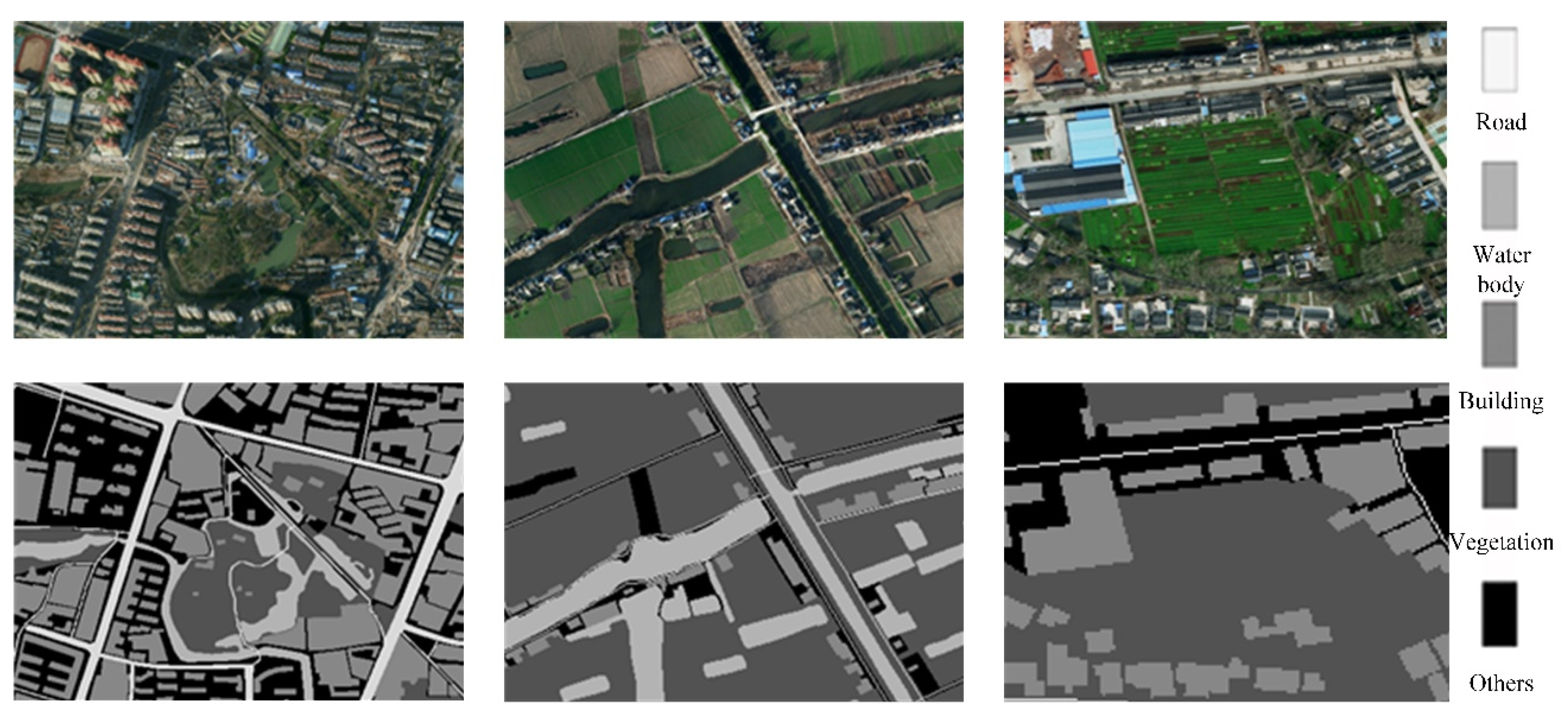
In this paper, we proposed a novel MFCSNet network for remote sensing image semantic segmentation. MFCSNet uses multi-scale deep features fusion and cost-sensitive loss function to make the segmentation network more effective. For the features extraction and fusion, MFCSNet provides a novel framework with multi-scale feature coding structure and max-pooling indices decoding structure. Instead of using FCN and SegNet, MFCSNet combines the corresponding down-sampling feature maps during up-sampling process to extract the low-level and high-level fusion features. Different U-Net framework, max-pooling indices decoding is used for up-sampling process, which can retain objects location information. This up-sampling structure can improve the recognition rate of the object edge. In MFCSNet, the batch normalization acceleration layer can reduce the sensitivity of the learning rate and improve the network convergence speed, which can make the network parameters optimize easily. To improve the classification performance on the category with a small number of samples, we design a cost-sensitive loss function by increasing the penalty for the misclassification of the object. For the MFCSNet model training, data enhancement and sample equalization processing are performed on the training set, which can suppress network overfitting and improve the generalization ability of the network. Compared with other state-of-the-art methods, i.e., U-Net and SegNet, the classification of all the objects with the proposed method has better classification accuracy. The precision of each category of MFCSNet has achieved the highest value. The OA and Kappa coefficient of MFCSNet is 94.46% and 0.9113, respectively, which are at least 1.92% and 0.0303 higher than U-Net and SegNet. Besides, the integrity of each object segmented by MFCSNet is obviously better than the others, especially road. Thus, the proposed MFCSNet can achieve promising performance in overall classification performance, feature edge recognition, consistency of prediction results, and so on.

Although our algorithm achieves promising semantic segmentation accuracy for the Jiage data set, there are some drawbacks and interesting ideas which can be further explored to extend the research reported in this paper. The segmentation of MFCSNet is based on the single pixel, which makes the contour information of the object not complete and the associated information between the objects lost. Thus, for the proposed method, the segmentation of some small roads is not complete, and there are some noisy pixels. Besides, in the test phase of this method, the large-size image needs to be divided into small blocks for testing. The test results are spliced to obtain the segmentation result of the original image. This can result in unevenness in the splice regions. In the future, the higher-order potentials, which constructed by different constraints based on the object structure information, the adjacency of pixels and topologies of different levels of segmentation regions will be introduced to construct the CRF model to optimize the rendering of the segmentation. In addition, some post-processing methods, such as morphological filtering, will also be used in the optimization of segmentation results.

References

1. Zhang, Y.; Yang, H.; Yuan, C. Overview of Remote Sensing Image Classification Methods. J. Ordnance Equip. Eng. 2018, 39, 108–112. [Google Scholar]
2. Gao, F.; Hilker, T.; Zhu, X.; Anderson, M.; Masek, J.; Wang, P.; Yang, Y. Fusing Landsat and MODIS Data for Vegetation Monitoring. IEEE Geosci. Remote Sens. Mag. 2015, 3, 47–60. [Google Scholar] [CrossRef]
3. Muller-Karger, F.; Roffer, M.; Walker, N.; Oliver, M.; Schofield, O.; Abbott, M.; Graber, H.C.; Leben, R.; Goni, G. Satellite remote sensing in support of an integrated ocean observing system. IEEE Geosci. Remote Sens. Mag. 2013, 1, 8–18. [Google Scholar] [CrossRef]
4. Qiong, Y.; Wei, L. Geological Exploration Scheme Based on Remote Sensing Image Processing Technology. In Proceedings of the 2016 IEEE International Conference on Smart Grid & Electrical Automation, Zhangjiajie, China, 11–12 August 2016. [Google Scholar]
5. Khatami, R.; Mountrakis, G.; Stehman, S.V. A meta-analysis of remote sensing research on supervised pixel-based land-cover image classification processes: General guidelines for practitioners and future research. Remote Sens. Environ. 2016, 177, 89–100. [Google Scholar] [CrossRef] [Green Version]
6. Bazi, Y.; Melgani, F. Gaussian Process Approach to Remote Sensing Image Classification. IEEE Trans. Geosci. Remote Sens. 2010, 48, 186–197. [Google Scholar] [CrossRef]
7. Hilker, T.; Hall, F.G.; Coops, N.C.; Collatz, J.G.; Black, T.A.; Tucker, C.J.; Sellers, P.J.; Grant, N.J. Remote sensing of transpiration and heat fluxes using multi-angle observations. Remote Sens. Environ. 2013, 137, 31–42. [Google Scholar] [CrossRef]
8. Palma, R.; Reznik, T.; Esbri, M.; Charvat, K.; Mazurek, C. An INSPIRE-Based Vocabulary for the Publication of Agricultural Linked Data. Ontol. Eng. Lect. Notes Comput. Sci. 2016, 9557, 124–133. [Google Scholar] [CrossRef]
9. Řezník, T.; Lukas, V.; Charvát, K.; Křivánek, Z.; Kepka, M.; Herman, L.; Řezníková, H. Disaster Risk Reduction in Agriculture through Geospatial (Big) Data Processing. ISPRS Int. J. Geo-Inf. 2017, 6, 238. [Google Scholar] [CrossRef]
10. Liu, Y.; Zhang, Z.; Zhong, R.; Chen, D.; Ke, Y.; Peethambara, J.; Chen, C.; Sun, L. Multi-level Building Detection Framework in Remote Sensing Images Based on Convolutional Neural Networks. IEEE J. Sel. Top. Appl. Earth Obs. Remote Sens. 2018, 11, 3688–3700. [Google Scholar] [CrossRef]
11. Liu, Y.; Yao, J.; Lu, X.; Xia, M.; Wang, X.; Liu, Y. RoadNet: Learning to Comprehensively Analyze Road Networks in Complex Urban Scenes From High-Resolution Remotely Sensed Images. IEEE Trans. Geosci. Remote Sens. 2019, 57, 2043–2056. [Google Scholar] [CrossRef]
12. Zhu, Q.; Zhong, Y.; Zhao, B.; Xia, G.S.; Zhang, L. Bag-of-Visual-Words Scene Classifier With Local and Global Features for High Spatial Resolution Remote Sensing Imagery. IEEE Geosci. Remote Sens. Lett. 2017, 13, 747–751. [Google Scholar] [CrossRef]
13. Swain, M.J.; Ballard, D.H. Indexing via Color Histograms. In Active Perception and Robot Vision; Sood, A.K., Wechsler, H., Eds.; Springer: Berlin/Heidelberg, Germany, 1992; pp. 390–393. [Google Scholar]
14. Qi, S.; Ma, J.; Lin, J.; Li, Y.; Tian, J. Unsupervised Ship Detection Based on Saliency and S-HOG Descriptor from Optical Satellite Images. IEEE Geosci. Remote Sens. Lett. 2015, 12, 1451–1455. [Google Scholar]
15. Lowe, D.G. Distinctive Image Features from Scale-Invariant Keypoints. Int. J. Comput. Vis. 2004, 60, 91–110. [Google Scholar] [CrossRef]
16. Wang, Y.; Mei, J.; Zhang, L.; Zhang, B.; Li, A.; Zheng, Y.; Zhu, P. Self-Supervised Low-Rank Representation (SSLRR) for Hyperspectral Image Classification. IEEE Trans. Geosci. Remote Sens. 2018, 56, 5658–5672. [Google Scholar] [CrossRef]
17. Xin, M.A.; Xiyuan, W.A.N.G.; Bo, H.U. Multi-source Remote Sensing Image Classification of CART Automatic Decision Tree Based on ENVI—Taking Beijing as an Example. Ningxia Eng. Technol. 2017, 16, 63–66. [Google Scholar]
18. Réjichi, S.; Chaabane, F. Feature extraction using PCA for VHR satellite image time series spatio-temporal classification. In Proceedings of the IEEE Geoscience and Remote Sensing Symposium 2015, Milan, Italy, 26–31 July 2015; pp. 485–488. [Google Scholar]
19. Zhao, Y.; Zhou, P. Application of Improved K-means Algorithm in Remote Sensing Image Classification. Remote Sens. Land Resour. 2011, 23, 87–90. [Google Scholar]
20. Hinton, G.E.; Salakhutdinov, R.R. Reducing the dimensionality of data with neural networks. Science 2006, 313, 504–507. [Google Scholar] [CrossRef] [PubMed]
21. LeCun, Y.; Bottou, L.; Bengio, Y.; Haffner, P. Gradient-based learning applied to document recognition. Proc. IEEE 1998, 86, 2278–2324. [Google Scholar] [CrossRef] [Green Version]
22. Krizhevsky, A.; Sutskever, I.; Hinton, G.E. ImageNet classification with deep convolutional neural networks. In Proceedings of the International Conference on Neural Information Processing Systems (NIPS), Lake Tahoe, NV, USA, 3–8 December 2012; pp. 1097–1105. [Google Scholar]
23. He, K.; Zhang, X.; Ren, S.; Sun, J. Deep Residual Learning for Image Recognition. In Proceedings of the IEEE Conference on Computer Vision and Pattern Recognition (CVPR), Las Vegas, NV, USA, 27–30 June 2016; pp. 770–778. [Google Scholar]
24. Girshick, R.; Donahue, J.; Darrell, T.; Malik, J. Rich feature hierarchies for object detection and semantic segmentation. In Proceedings of the IEEE Conference on Computer Vision and Pattern Recognition, Columbus, OH, USA, 23–28 June 2014; pp. 580–587. [Google Scholar]
25. Ren, S.; He, K.; Girshick, R.; Sun, J. Faster R-CNN: Towards real-time object detection with region proposal networks. In Proceedings of the International Conference on Neural Information Processing Systems (NIPS), Montreal, QC, Canada, 7–12 December 2015; pp. 91–99. [Google Scholar]
26. Liu, W.; Anguelov, D.; Erhan, D.; Szegedy, C.; Reed, S.; Fu, C.Y.; Berg, A.C. SSD: Single Shot MultiBox Detector. In Proceedings of the European Conference on Computer Vision (ECCV), Amsterdam, The Netherlands, 8–16 October 2016; pp. 21–37. [Google Scholar]
27. Redmon, J.; Divvala, S.; Girshick, R.; Farhadi, A. You Only Look Once: Unified, Real-Time Object Detection. In Proceedings of the IEEE Computer Vision and Pattern Recognition, Las Vegas, NV, USA, 26 June–1 July 2016; pp. 779–788. [Google Scholar]
28. Shelhamer, E.; Long, J.; Darrell, T. Fully Convolutional Networks for Semantic Segmentation. In Proceedings of the IEEE Transactions on Pattern Analysis Machine Intelligence, Boston, MA, USA, 7–12 June 2015; pp. 3431–3440. [Google Scholar]
29. Badrinarayanan, V.; Kendall, A.; Cipolla, R. SegNet: A Deep Convolutional Encoder-Decoder Architecture for Scene Segmentation. IEEE Trans. Pattern Anal. Mach. Intell. 2017, 39, 2481–2495. [Google Scholar] [CrossRef] [PubMed]
30. Ronneberger, O.; Fischer, P.; Brox, T. U-Net: Convolutional Networks for Biomedical Image Segmentation. In Proceedings of the Medical Image Computing and Computer-Assisted Intervention—MICCAI 2015, Munich, Germany, 5–9 October 2015; pp. 234–241. [Google Scholar]
31. Yu, F.; Koltun, V. Multi-Scale Context Aggregation by Dilated Convolutions. In Proceedings of the International Conference on Learning Representations (ICLR), San Juan, Puerto Rico, 2–4 May 2016; pp. 1–9. [Google Scholar]
32. Cao, L.; Li, H.; Han, Y.; Yu, F.; Gu, H. Application of Convolutional Neural Networks in Classification of High Score Remote Sensing Images. J. Surv. Mapp. 2016, 41, 170–175. [Google Scholar]
33. Maggiori, E.; Tarabalka, Y.; Charpiat, G.; Alliez, P. Fully convolutional neural networks for remote sensing image classification. In Proceedings of the 2016 IEEE Geoscience and Remote Sensing Symposium, Beijing, China, 10–15 July 2016; pp. 5071–5074. [Google Scholar]
34. Agoub, A.; Filippovska, Y.; Schmidt, V.; Kada, M. Automatic Generation of Photorealistic Image Fillers for Privacy Enabled Urban Basemaps using Generative Adversarial Networks. In Proceedings of the 29th International Cartographic Conference (ICC 2019), Tokyo, Japan, 15–20 July 2019. [Google Scholar]
35. He, M.; Li, X.; Zhang, Y.; Zhang, J.; Wang, W. Hyperspectral image classification based on deep stacking network. In Proceedings of the 2016 IEEE Geoscience and Remote Sensing Symposium, Beijing, China, 10–15 July 2016; pp. 3286–3289. [Google Scholar]
Figure 1. U-Net network structure. Note that the figure is designed according to Reference [30].
Applsci 09 04043 g001
Figure 2. SegNet network structure. Note that the figure is designed according to Reference [29].
Applsci 09 04043 g002
Figure 3. The proposed network structure.
Applsci 09 04043 g003
Figure 4. Max-pooling indices and deconvolution up-sampling.
Applsci 09 04043 g004
Figure 5. Partial training set and labels.
Applsci 09 04043 g005
Figure 6. Part of the cutting images in the training set.
Applsci 09 04043 g006
Figure 7. Data augmentation examples.
Applsci 09 04043 g007
Figure 8. Different categories of sample statistics in the data set.
Applsci 09 04043 g008
Figure 9. Image preprocessing flowchart.
Applsci 09 04043 g009
Figure 10. Experimental results of different remote sensing image classification algorithms.
Applsci 09 04043 g010