Research on Low Energy Consumption Static Postures of Bionic Feet

Abstract

By studying the relation of the robot’s postures and its energy consumption, a static analysis-based method to obtain the low-energy postures of the robot is proposed. This method decreases the energy consumption and increases the battery life by adjusting the postures in the horizontal environment. The method takes the low-speed hexapod bionic robot as the research object. First, we obtain the output torque of each joint of the leg through static analysis and establish the energy consumption model of the robot. Considering the flexibility of the robot, we then introduce the performance index of the maximum step length and establish an equilibrium solution based on energy consumption and maximum step size. Finally, we derive the low-energy postures of the robot using MATLAB (MATLAB 2014a, The MathWorks, Natick, Massachusetts State, USA, 2014) simulations. An energy consumption experiment is carried out with a physical prototype to verify the validity of the method.

1. Introduction

As an important branch of the mobile robot field, the robot with feet has good mobility, environmental adaptability, high research value and broad application prospects. However, in the actual operation of such robots, there are many shortcomings, such as low energy efficiency and high energy consumption. Especially in the low-speed mobile operation with high stability and heavy load, the robot spends more electricity in the stationary state, during which it needs to maintain its body level and other specific functions, such as positioning, loading, and fixed-point operation. The energy consumption under this non-moving state cannot be neglected [1,2,3]. By observing the standing state of spiders, stick insects, and other polypods in different environments, robots with feet should have a low energy consumption posture that meets certain constraints.

Many scholars have conducted research on the energy consumption of robots with feet and reduced the energy consumption through a joint locking device; however, this device brings additional energy consumption and cumbersome mechanism problems [4,5,6]. Shibendu et al. [7,8,9] used the Lagrangian–Eulerian dynamic equation to establish the robot’s system and used the least-squares method to obtain the joint torque and optimize the trajectory; then, they analyzed the energy consumption under the robot’s motion state. Erden et al. [10,11,12] used the Newton–Euler method to further optimize the static heat loss of the robot, proposed an optimal allocation method for each torque of the hexapod robot, and used computer simulations to evaluate the energy consumption of the robot system to reduce energy consumption. Pablo et al. [13,14,15] obtained the optimal configuration of the robot leg structure by analyzing the influence of different configurations of hexapod robot legs on the energy consumption of the robot system; they effectively reduced the system’s energy consumption. Chen Xuedong et al. [16,17] used foot force distribution as the breakthrough point in the study of quadruped robots and realized the optimization of torque distribution and energy consumption of the system.

Jin Bo and Chen Cheng [18,19,20] built a dynamic model of a robot with feet, got the relationship between the joint torque and the force on the foot, and considered the power and heat loss of the driver to optimize the distribution of the joint moment; thus, they obtained the walking mode of the robot with minimum energy consumption. Li Yibin et al. [21,22,23] explored the influence of robot posture on motion from the posture of the quadruped robot. The existing energy consumption analysis methods mentioned above are mainly aimed at energy consumption analysis and optimization of different leg configurations under the motion state of robots with feet and rarely involve energy consumption analysis of the robot in the static posture.

The ideas presented in this article originate from "bionics", and it was hoped that by analysis, a standing posture that mimicked similar insects or four-legged animals could be proposed, which was based on the natural attitude choices of energy-efficient insects or animals. This paper took a self-customized low-speed hexapod robot as the research object, also known as the spider robot, which is a kind of multi-foot robot. The hexapod robot is expected to mimic the insect’s movement organs and motor principles, as well as the gaits. Incorporating superior biological properties into the design of the robot gives the robot superior performances, flexibility, adaptability and maneuverability. Compared with other bionic robots, the foot-type bionic robot has the advantages of discrete footsteps, flexible movement, obstacle-avoidance ability and terrain adaptability. It can be flexibly and stably integrated into unstructured terrains such as sands and grassland. The hexapod robot is a representative type of foot bionic robot, which not only has the characteristics common to the foot robot, but also has high joint redundancy and high stability compared with biped and quadruped robots. This makes it more flexible, maneuverable and autonomous when moving in unknown, complex terrain environments.

Aiming at the above problems, this paper took the low-speed hexapod bionic robot as the research object and proposed a low-energy posture analysis method in the static state. By establishing the dynamic relationship between the robot’s posture change and energy consumption of the robot, the goal of reducing energy consumption and prolonging the battery life was achieved. First, through the kinematics and static analysis of the robot, the overall energy consumption model of the robot was established. Considering the motion flexibility of the robot, the maximum step objective function of the robot was designed. Second, based on the minimum energy consumption target and the maximum step size, computer simulations were used. Finally, the correctness and effectiveness of the proposed method were verified by an energy consumption experiment with a prototype robot, and the natural standing posture similar to insects was obtained, which achieved the goal of reducing energy consumption.

2. The Kinematics and Static Analysis of a Hexapod Robot

The energy consumption of the robot in the static state was not only related to its own gravity, joint driving force, and foot reaction force but also related to the postures of the robot. The factors affecting the posture included the height of the body and the joint angle of the legs. Through the kinematics and static analysis of the robot, the model between the postures and energy of the robot was established, and the method for obtaining low-energy postures under unconstrained conditions was obtained.

2.1. Kinematics Analysis

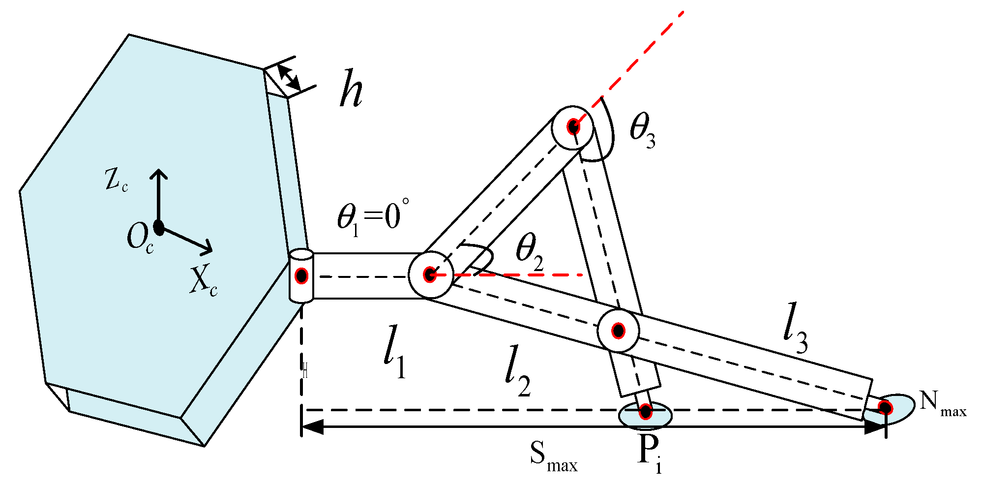
The MDH (The Matrix of Denavit-Hartenberg) method was used to establish the one-legged model of the hexapod robot. The relationship between the angle of leg joint rotation and the position of the foot tip was given by kinematics analysis of the robot. The joint structure of the right middle leg of the robot is shown in Figure 1. The parameters are defined in

Table 1. Description of parameters in Figure 1.

Parameter	Description
$O_c-X_c{Y}_c{Z}_c$	Robot body coordinate system
$\begin{array}{l}{O}_j-X_j{Y}_j{Z}_j\\ (j=1,2,3,4)\end{array}$	Coordinates of the robot heel joint, hip joint, knee joint, and foot tip.
$l_k(k=1,2,3)$	Lengths of the three joints of the robot’s legs
${\theta }_k(k=1,2,3)$	Corners of the three joints of the robot’s legs
$G$,$G^{\prime }$	Total body weight and load weight
$P_i\{P_{ix}$,$P_{iy}$,$P_{iz}\}$ $(i=1,2,\cdots ,6)$	Position of the robot’s foot tip in the joint coordinate system
$F\text{{}{f}_{ix,}{f}_{iy,}{f}_{iz}\}$ $(i=1,2,\cdots ,6)$	Reaction force of the robot’s foot tip

. The MDH parameters of the leg joint are shown in

Table 2. MDH parameters of the right-middle leg.

Joint Number	${\mathit{\theta }}_{\mathit{k}}$	${\mathit{\alpha }}_{\mathit{k}}$	${\mathit{l}}_{\mathit{k}}$	${\mathit{d}}_{\mathit{k}}$
1	${\theta }_c$	0	$l_c$	0
2	${\theta }_1$	$\pi /2$	$l_1$	0
3	${\theta }_2$	0	$l_2$	0
4	${\theta }_3$	0	$l_3$	0

. Among them, $l_k$ represents the length of the rods in each joint of the robot leg, ${\alpha }_k$ represents the corresponding torsion angle of the rods, $d_k$ represents the distance of the joints, and ${\theta }_k$ represents the rotation angle of the joints.

According to the homogeneous transformation matrix formula, the pose transformation matrix of the robot foot relative to the heel joint coordinate system is as follows:

$${}^{c}T{}_4={}^{c}T_1{}^{1}T{}_2{}^{2}T{}_3{}^{3}T{}_4=\left[\begin{array}{cccc}{c}_1{c}_2{c}_3-c_1{s}_2{s}_3& -c_1{c}_2{s}_3-c_1{s}_2{c}_3& -s_1& l_1{c}_1+l_2{c}_1{c}_2+l_3{c}_1{c}_{23}+b/2\\ s_1{c}_2{c}_3-s_1{s}_2{s}_3& -s_1{c}_2{s}_3-s_1{s}_2{c}_3& c_1& l_1{s}_1+l_2{s}_1{c}_2+l_3{s}_1{c}_{23}\\ -s_2{c}_3-c_2{s}_3& s_2{s}_3-c_2{c}_3& 0& l_2{s}_2+l_3{s}_{23}\\ 0& 0& 0& 1\end{array}\right],$$

(1)

where $s_1$ represents ${\mathit{sin}\theta }_1$, $c_1$ represents ${\mathit{cos}\theta }_1$, $c_{23}$ represents ${\mathit{cos}(\theta }_2{+\theta }_3)$, $s_{23}$ represents ${\mathit{sin}(\theta }_2{+\theta }_3)$, and $b$ represents the distance between the heel joints of the robot’s two middle legs. The position of the foot tip in the coordinate system of the heel joint is

$$P_i={[\begin{array}{ccc}{P}_{ix}& P_{iy}& P_{iz}\end{array}]}^T=\left[\begin{array}{c}{l}_1{c}_1+l_2{c}_1{c}_2+l_3{c}_1{c}_{23}+b/2\\ l_1{s}_1+l_2{s}_1{c}_2+l_3{s}_1{c}_{23}\\ l_2{s}_2+l_3{s}_{23}\end{array}\right].$$

(2)

Its Jacobian matrix is

$$J=\left[\begin{array}{ccc}-s_1(l_3{c}_{23}+l_2{c}_2+l_1)& c_1(-l_3{s}_{23}-l_2{s}_2)& -l_3{c}_1{s}_{23}\\ c_1(l_3{c}_{23}+l_2{c}_2+l_1)& s_1(-l_3{s}_{23}-l_2{s}_2)& -l_3{s}_1{s}_{23}\\ 0& -l_3{c}_{23}-l_2{c}_2& -l_3{c}_{23}\end{array}\right].$$

(3)

By solving the inverse kinematics equation, the joint angles of the robot can be obtained:

$$\{\begin{array}{l}{\theta }_1=\arctan (\frac{P_y}{P_x})\\ {\theta }_2=-\arccos (\frac{P_z}{\sqrt{K^2+L^2}})-\psi \\ {\theta }_3=\arccos (\frac{B^2+P_z{}^2-l_2{}^2-l_3{}^2}{2l_2{l}_3})\end{array},$$

(4)

where

$$\begin{array}{l}K=l_2+l_3{c}_3,L=l_3{s}_3,\\ \psi =\arcsin (\frac{K}{\sqrt{K^2+L^2}}),B=\frac{P_x}{c_1}-l_1\end{array}$$

The inverse kinematics Equation (4) of the robot is abbreviated as follows:

$${\theta }_k=K_I(P_i).$$

(5)

2.2. Static Analysis

The energy consumption of the robot in the static posture was mainly derived from the torque generated by the leg joint actuator to overcome the weight of the machine and the load gravity it received. Without considering the loss, the motor torque could be simplified by the joint torque expression, and the low energy consumption analysis model of the robot could be established from the sum of the joint torque values of all the support legs. When the robot was stably static, the main force was concentrated on the $X_1{O}_1{Z}_1$ plane of the coordinate system ${\mathsf{\Sigma }O}_1$, and the torso force of the simplified robot was at the origin of the coordinate system. It can be seen from the analysis of Figure 1 that the change in joint angle ${\theta }_1$ affected the length of the force arm of each joint, and the change in joint angle ${\theta }_2{,\theta }_3$ had an influence on the height of the body’s center of gravity. We established the relationship between the joint torque of the leg and the force exerted on the foot, as shown in Equation (6):

$${\tau }_i=J^{T}F(i=1,2,\cdots ,6).$$

(6)

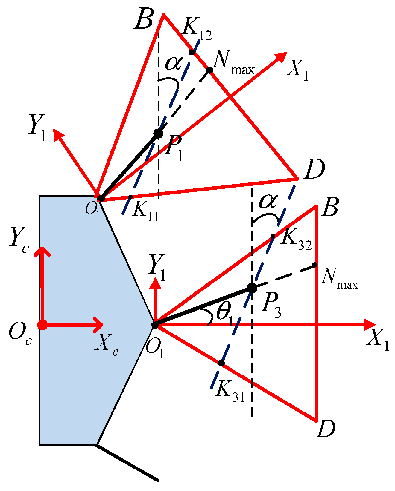
Assuming that the robot is loaded, the center of gravity of the body remains unchanged, and the body can be kept horizontal and static by adjusting the foot position of the supporting leg. The contact of the foot tip with the ground can be modeled as a hard point contact with friction, which indicates that the interaction between the foot tip and the ground is limited to three force components [24], as shown in the enlarged portion of Figure 1. Force $f_{iz}$ is in the vertical direction, and forces $f_{ix}$ and $f_{iy}$ are in the ground direction. The force at the foot of each leg can be expressed as follows:

$$AF=-BW,$$

(7)

where

$$W={\left[F_x{,F}_y{,F}_z{,M}_x{,M}_y{,M}_z\right]}^T.$$

When $\beta =1/2$, $\mathrm{A}={\left[\begin{array}{ccc}{I}_3& I_3& I_3\\ R_p& R_q& R_r\end{array}\right]}_{6\times 9}$;

when $\beta =2/3$, $\mathrm{A}={\left[\begin{array}{cccc}{I}_3& I_3& I_3& I_3\\ R_p& R_q& R_r& R_s\end{array}\right]}_{6\times 12}$;

when $\beta =5/6$, $\mathrm{A}={\left[\begin{array}{ccccc}{I}_3& I_3& I_3& I_3& I_3\\ R_p& R_q& R_r& R_s& R_t\end{array}\right]}_{6\times 15}$;

$\mathrm{B}={\left[\begin{array}{cc}{I}_3& 0_3\\ R_c& I_3\end{array}\right]}_{6\times 6}$; $R_i=\left[\begin{array}{ccc}0& –z_i& y_i\\ z_i& 0& {-x}_i\\ {-y}_i& x_i& 0\end{array}\right]$ and $I_3=\left[\begin{array}{ccc}1& 0& 0\\ 0& 1& 0\\ 0& 0& 1\end{array}\right]$.

$\beta$ is the duty cycle of the robot; $I_3$ is the unit matrix of $3\times 3$; $0_3$ is the unit matrix of $3\times 3$; $R_i$ is the oblique symmetric matrix of vector ${{[x}_i{,y}_i{,z}_i]}^T$; and ${[x}_i{,y}_i{,z}_i{]}^T$ is the position coordinate of the foot tip relative to the coordinate system of body’s center of gravity.

Here, $R_i=\left[\begin{array}{ccc}0& {-z}_i& y_i\\ z_i& 0& {-x}_i\\ {-y}_i& x_i& 0\end{array}\right]$. These matrices define the position of the foot relative to the reference coordinate system of the body’s center of gravity (for $\beta =1/2$, $i=p,q,r$; for $\beta =2/3$, $i=p,q,r,s$; for $\beta =5/6$, $i=p,q,r,s,t$). We define the overall energy consumption model of the robot as follows:

$$M={\displaystyle \sum _{i=1}^6\left|{\tau }_i\right|}.$$

(8)

We solved the minimum value of M within the limited range of the robot structure and obtained the corresponding center of gravity height H and the joint angles of legs ${\theta }_i$. Defining the low-energy postures $Pose=\left\{{H,\theta }_i\right\}(i=1,2,3)$ determined the low-energy static posture of the robot under unconstrained conditions.

3. Experimental Platform

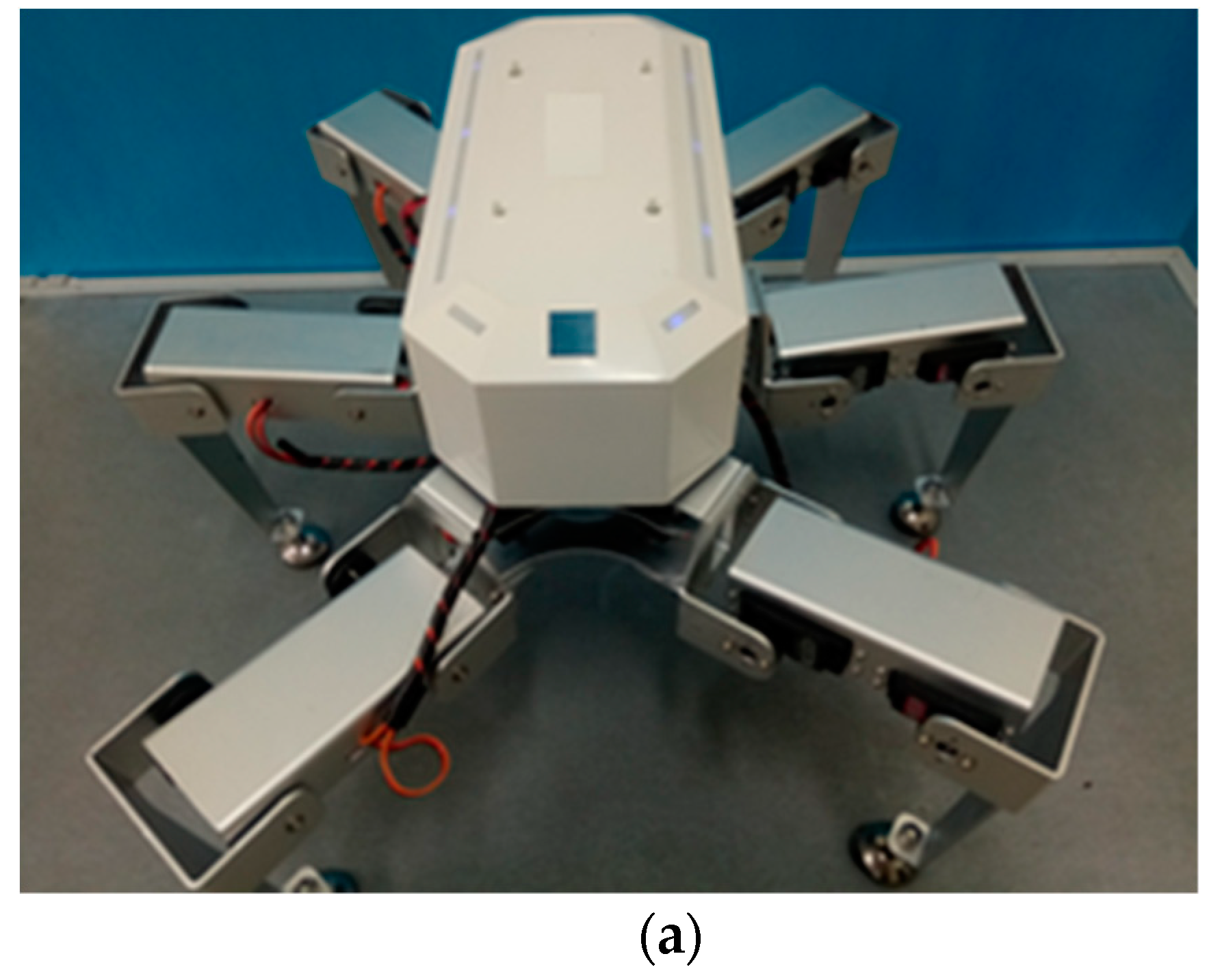
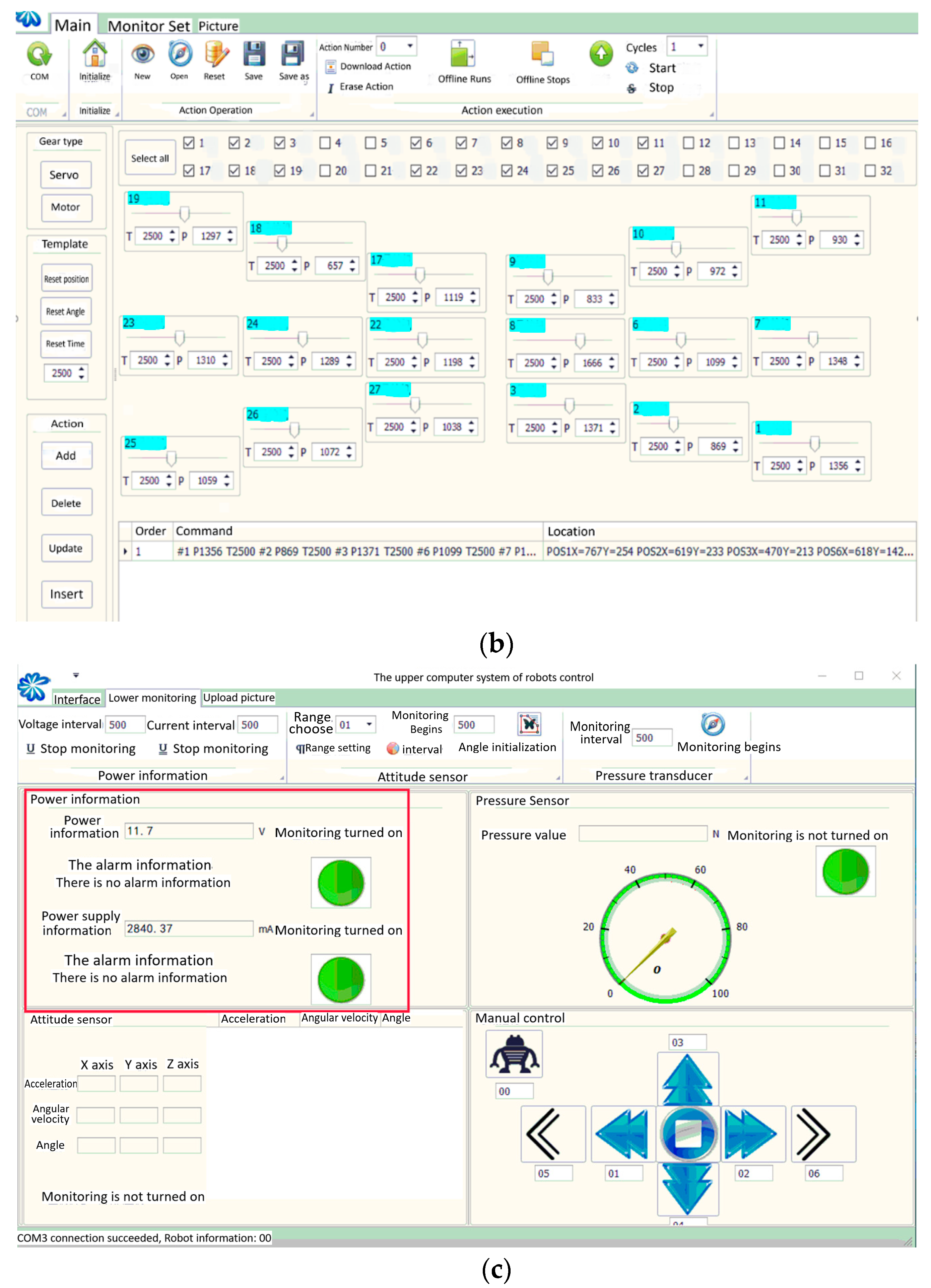
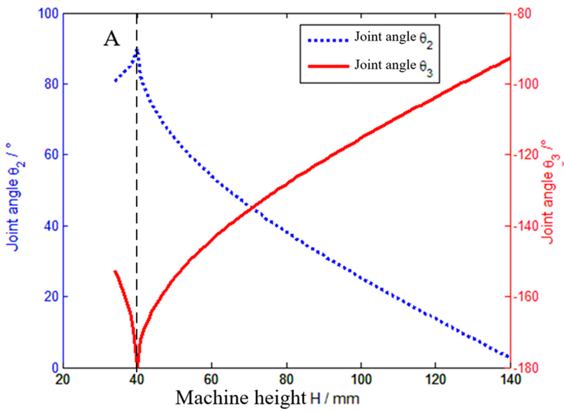
In this paper, the self-developed hexapod robot was used as the simulation and experimental object. The prototype and the upper computer software used in the experiment are shown in Figure 2 [25,26]. Each leg of the robot consisted of three limb joints and three rotating joints, which were driven by digital servos and allowed current feedback. The foot tips adopted a universal joint structure with a restricted position. Figure 2b shows the servo control interface, mainly used for setting the posture of the robot. Figure 2c shows the monitoring interface of the lower computer, which was mainly used to monitor the total current of the robot system in real time. The specific structural parameters of the robot are shown in

Table 3. Structural parameters of the robot.

Parameter	Value	Parameter	Value
$l_1 \left[\mathrm{mm}\right]$	75	$G\left[\mathrm{kg}\right]$	2.144
$l_2 \left[\mathrm{mm}\right]$	105	${\theta }_1$$[\mathrm{deg}]$	−45 – 45
$l_3 \left[\mathrm{mm}\right]$	145	${\theta }_2$$[\mathrm{deg}]$	−45 – 90
$G^{\prime }$ [kg]	1.0	${\theta }_3$$[\mathrm{deg}]$	−180 – 0
$H$$\left[\mathrm{mm}\right]$	30–140	h$\left[\mathrm{mm}\right]$	28

.

An RFP602 force sensor was used in the experiment. Its feedback value was voltage, and the corresponding voltage was proportional to the magnitude of force. The measured voltage value was converted into a foot force ${F(f}_{ix}{,f}_{iy}{,f}_{iz})$ and was substituted into Equation (6) to obtain the torque of each joint. Equation (7) was used to obtain the pose and energy consumption of the robot at any given time. The experimental measurements showed that although the force acting on the foot was different at different landing points, the trend of change in force was similar. In order to simplify the calculation, the average $F=(G+G^{\prime })/6$ was used as the simulation data, and $G^{\prime }$ was the load mass.

Here, H is the height range of the machine’s center of gravity from the ground, and h is the thickness of the body.

4. Static Posture Analysis Considering Energy Consumption Target Only

The minimum energy consumption of the robot in the static posture was analyzed by the overall energy consumption model of the robot established in the previous section. The analysis of the robot was without any posture constraints and only considered the situation of the lowest energy consumption. When the body of the robot touched the ground, that was, when $H=0$, the supporting force was provided by the ground, and it was not necessary to provide a driving force. At this time, the robot could not continue to move, and it needed to perform additional actions to return to a certain height before it could work normally. Therefore, this state was not be studied in this paper.

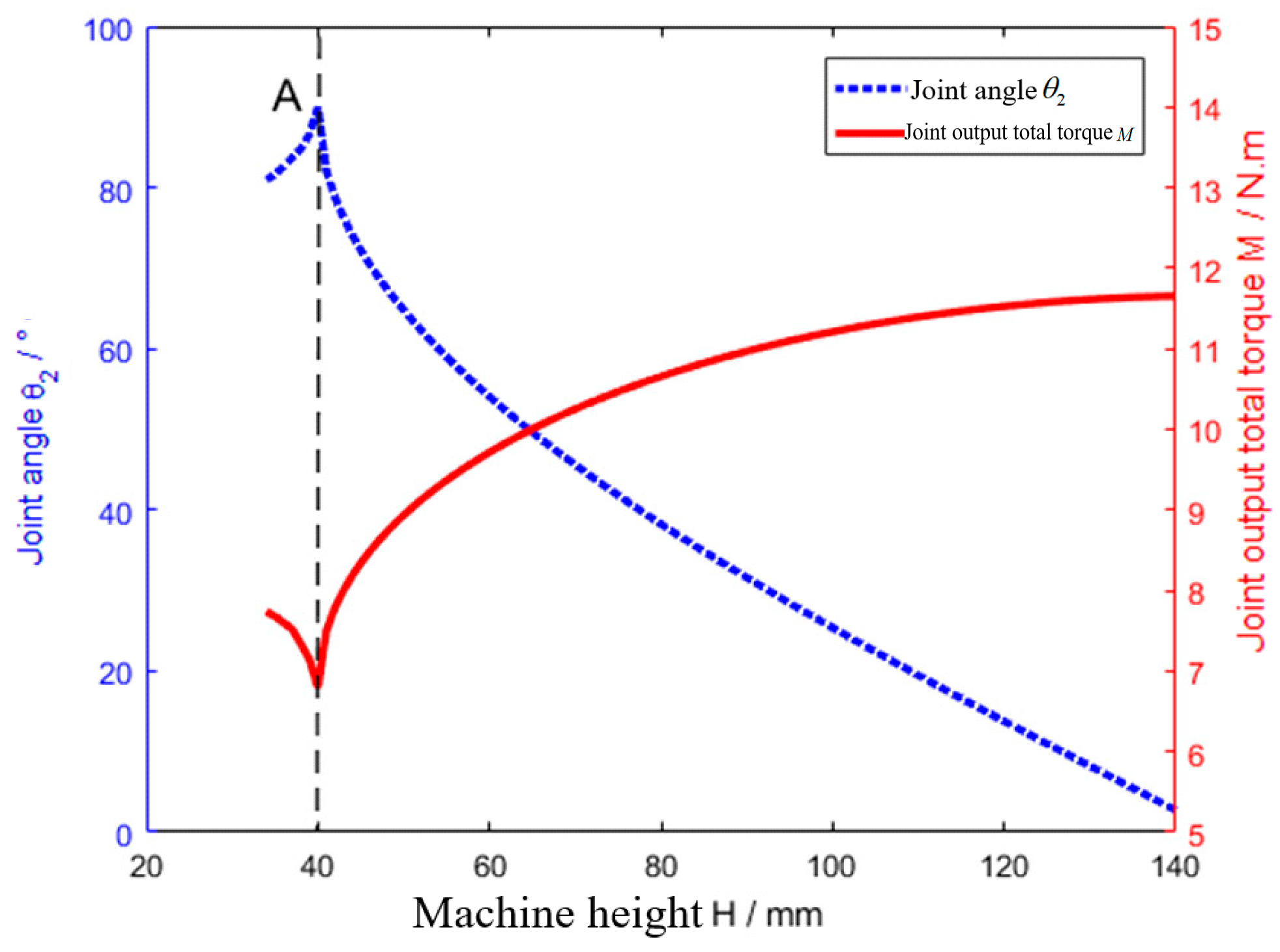
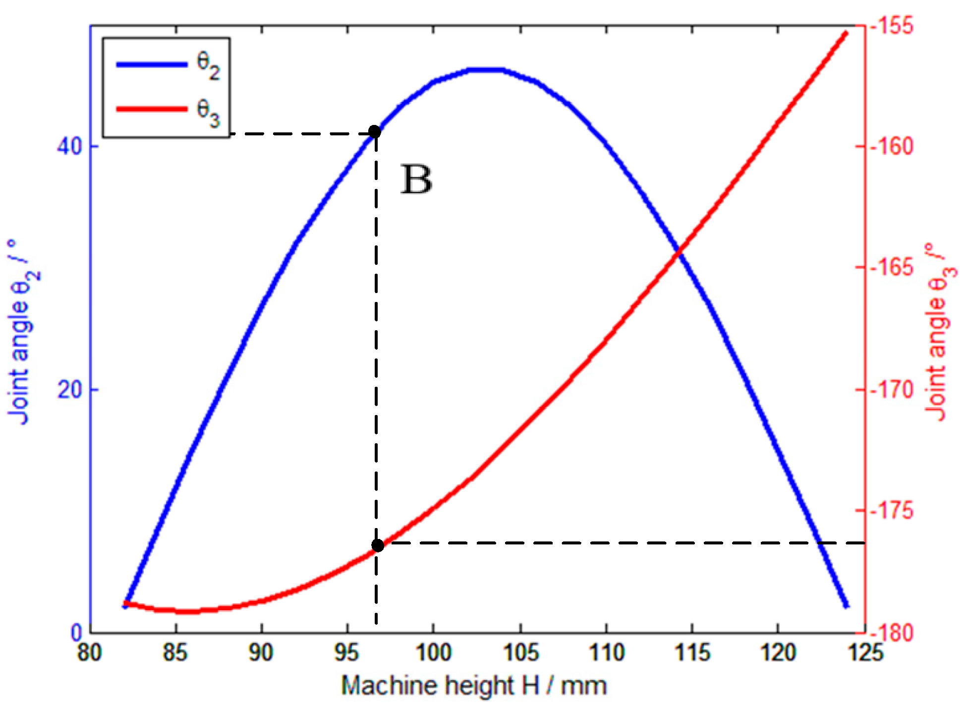
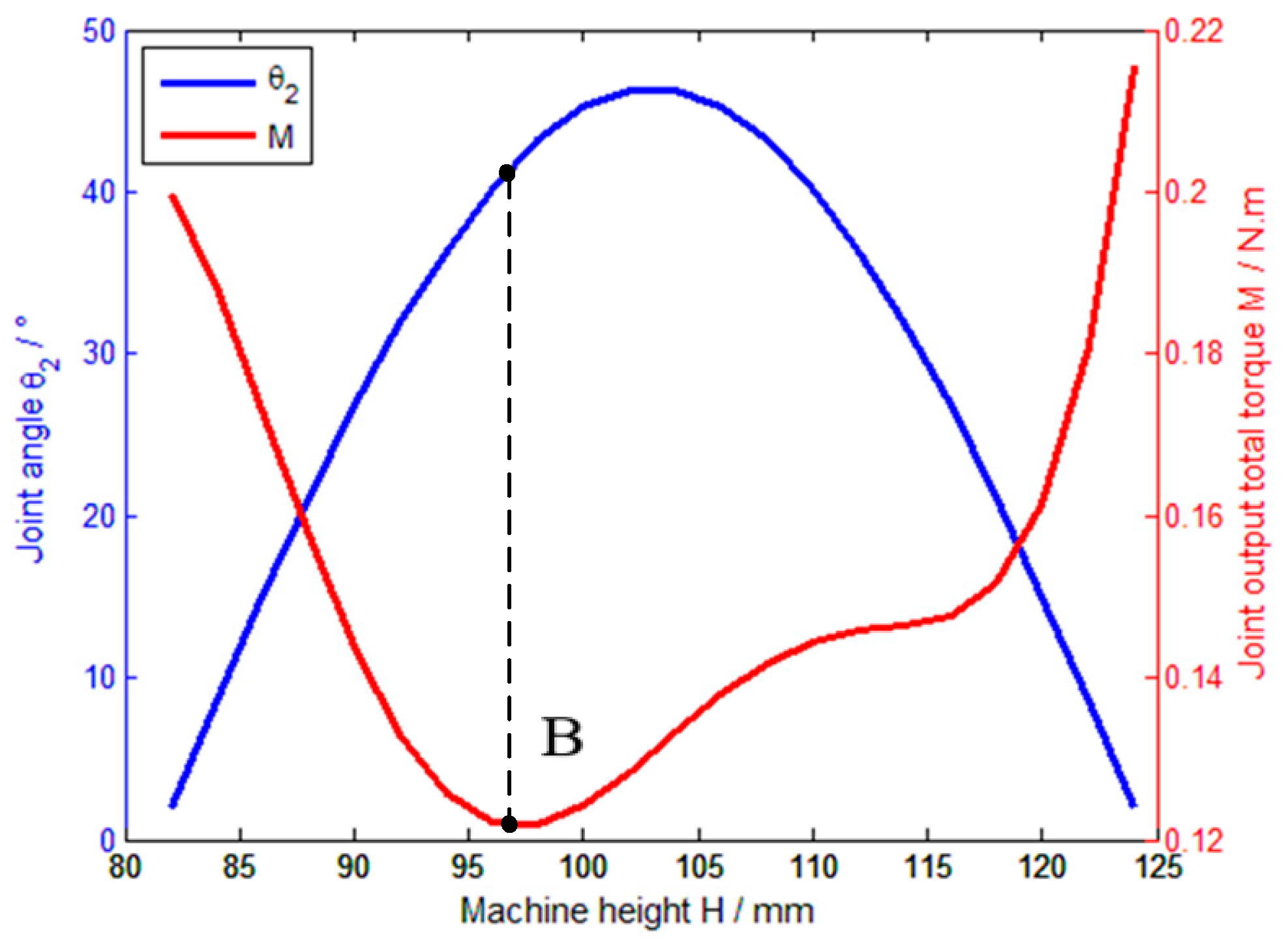
When $H\ne 0$, the minimum energy consumption posture of the robot in the static posture was verified by simulation. First, we set the joint angle ${\theta }_1{=0}^{°}$ and the yaw angle ${\alpha =0}^{°}$. We followed the steps below in the simulation. (1) Using the robotic toolbox of MATLAB, the D–H model and the data in Table 3 were used to establish a single-leg model. (2) According to the joint range of the mechanical structure of the robot body, we calculated the nearest landing point and the farthest landing point of the robot’s single leg. (3) We drew a straight line as a foot trajectory with two landing points (obtained in step (2) as the starting point and the end point). (4) We took out some points of the fixed interval in the trajectory as the foot position, and the corresponding joint angle during the movement of the single leg was obtained from the foot position through kinematic inversion. (5) We solved the corresponding Jacobian matrix J. (6) By substituting the full force $\mathrm{F}$ and the Jacobian matrix $J$ into Equation (6), the joint angles ${\theta }_2$ and ${\theta }_3$ of the leg when the total output torque $M$ of the joint was minimum could be obtained under different center of gravity heights $H$. The corresponding minimum joint output total torque $M$ values are shown in Figure 3 and Figure 4.

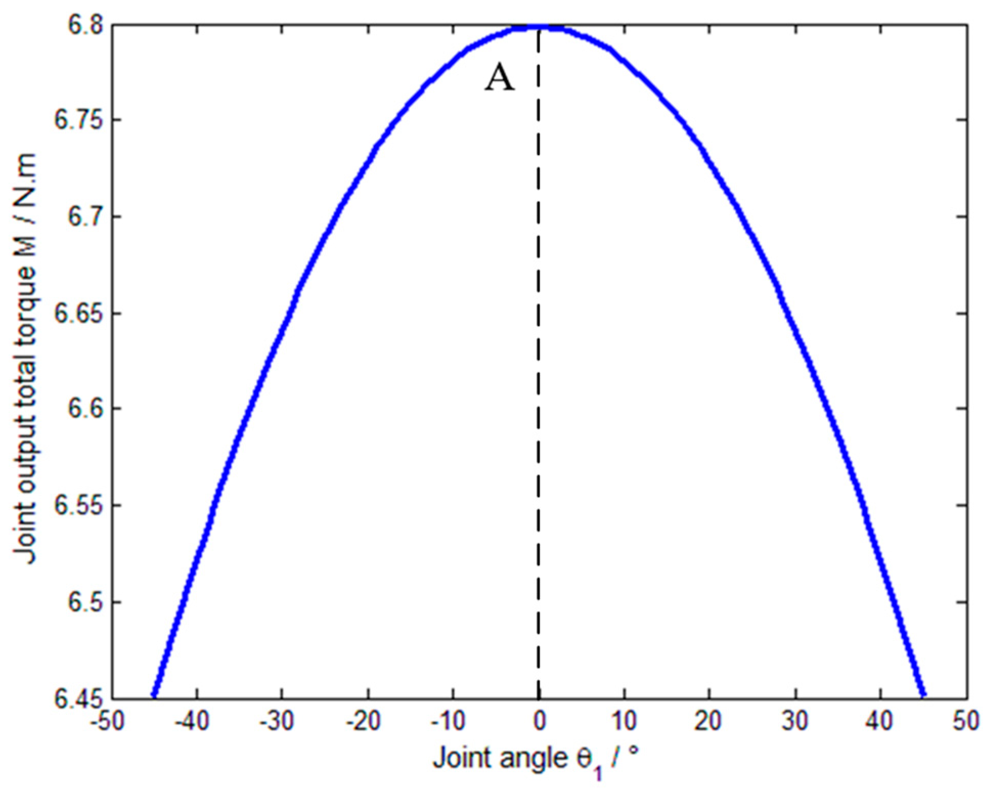
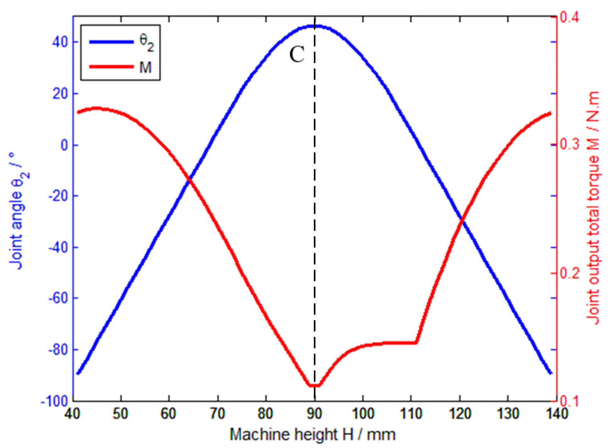
It can be seen from Figure 3 and Figure 4 that when the joint angle was fixed, and when only the energy consumption target was considered, the total output torque of the joint was the smallest within the limit of the robot’s center of gravity, that was, at point A in Figure 4. At this time, the hexapod robot’s static posture was as follows:

$$H=40.0\left[\mathrm{mm}\right]{,\theta }_1{=0}^{°}{,\theta }_2={90.0}^{°}{,\theta }_3= –{180.0}^{°}.$$

Next, by changing the value of joint angle ${\theta }_1$, the relationship curve between joint angle ${\theta }_1$ and the joint output total torque M was obtained, as shown in Figure 5.

Combining Figure 4 and Figure 5, in the case of considering only the energy consumption target, within the range of the joint angle ${\theta }_1$, the low-energy static posture of the robot was as follows, and the actual robot posture was the posture ① and the postures ②:

$$H=40.0\left[\mathrm{mm}\right]{,\theta }_1={45.0}^{°}{,\theta }_2={90.0}^{°}{,\theta }_3=-{180.0}^{°},$$

$$H=40.0\left[\mathrm{mm}\right]{,\theta }_1=-{45.0}^{°}{,\theta }_2={90.0}^{°}{,\theta }_3=-{180.0}^{°}.$$

5. Static Postures Analysis Considering Energy Consumption and Maximum Step Size

5.1. Maximum Step Constraint

Due to the high redundancy of the hexapod robot, multiple sets of solutions can be obtained with a certain center of gravity height and position of the foot tip. When the extreme value was solved, the singular postures were obtained within the mechanical limits of the robot. For example, for the robot’s legs close to the body trunk, the static energy of the robot was low, and the flexibility of movement was lost. In addition, the resulting low energy consumption posture was not unique.

Based on the analysis of joint torque, this paper comprehensively considered the motion characteristics of the robot from the static state to the motion state. By adopting the maximum step size and increasing the constraints of the robot postures, the movable range of the joints of the robot legs was further restricted, thereby obtaining an effective low-energy posture.

Reachable Area of the Robot Foot

For ease of calculation, the reachable area of the robot’s foot tip was replaced by an equilateral triangle BOD, as shown in Figure 6. The area was related to the robot’s center of gravity height $\mathrm{H}$, and the parameters are defined in

Table 4. The maximum step size of parameters.

Parameter	Description
${\theta }_1$	Angle between the robot leg and the coordinate axis $X_1$
$\alpha$	Yaw angle of the robot, indicating the ability of the robot to move in one direction
${\mathrm{N}}_{\max }$	The farthest point that the robot’s foot can reach
$K_{i1,}{K}_{i2}$	The intersection of the direction of the $i$ leg of the robot and the boundary of the reachable area
$\mathrm{H}$	Robot’s center of gravity height

.

5.2. Foot Tip Landing Points in the Movable Area

The position of the landing point can be obtained by calculation:

$${\mathrm{p}}_{\mathrm{i}}=\left[\mathrm{d},0,-\mathrm{H}\right],$$

where

$$d=\left(l_1+\sqrt{{\left(l_2{+l}_3\right)}^2{-H}^2}\right).$$

According to Figure 6, when the landing point was at the midpoint of the movable area, the yaw angle ${\alpha =0}^{°}$, the joint angle ${\theta }_1{=0}^{°}$, and the robot load $G^{\prime }$ = 1.0 [kg]. First, when the robot is at a different center of gravity H, the leg joint angles ${\theta }_2$ and ${\theta }_3$ that minimize the joint output total moment M and the corresponding minimum joint output total torque M are obtained, and are shown in Figure 7 and Figure 8, respectively.

When the foot point $p_i$ fell in the midpoint of the movable area, the low energy consumption static posture of the robot was within the constraint range of the joint angle ${\theta }_1{=0}^{°}$, and the low-energy static postures of the robot was at point $B$:

$$H=97.0\left[\mathrm{mm}\right]{,\theta }_1{=0}^{°}{,\theta }_2={43.13}^{°}{,\theta }_3= {-176}^{°}.$$

5.3. Given the Yaw Angle $\alpha$, the Foot Tip Falls in the Middle of the Maximum Step Size

5.3.1. Maximum Step Analysis of the Robot

The maximum step $R_i$ of a single leg is the maximum distance between a certain direction and the intersection with the movable area. It is assumed that in the joint coordinate system, the coordinate of $K_{i1}$ is ${(x}_{i1}{,x}_{i2}{,x}_{i3})$, the coordinate of $K_{i2}$ is ${(y}_{i1}{,y}_{i2}{,y}_{i3})$, and the maximum step size is obtained by Equation (9):

$$R_i=\left|K_{i1}{K}_{i2}\right|=\sqrt{{\left(x_{i1}{-x}_{i2}\right)}^2+{\left(y_{i1}{-y}_{i2}\right)}^2+{\left(z_{i1} –z_{i2}\right)}^2}.$$

(9)

At any joint angle, the single-leg support state of the robot is shown in Figure 9, where $h$ is the thickness of the robot body.

According to the geometric relationship, the following constraint equation can be established:

$${H=-l}_2{s}_2 -l_3{s}_{23}.$$

(10)

Equation (9) is the postures constraint equation of the robot used to define the effective range of the joints of the robot legs, and $H$ is a function of ${\theta }_2$, ${\theta }_3$. According to the trunk structure and leg structure of the robot, the range of $H$, that is, $H\in [\frac{h}{2}{,l}_2{+l}_3]$, can be determined.

Assuming that the yaw angle $\alpha$ and the center of gravity height $\mathrm{H}$ are known, the coordinates of the two points ${\mathrm{K}}_{\mathrm{i}1}$ and ${\mathrm{K}}_{\mathrm{i}2}$ are obtained by the following kinematic equation:

$$\{\begin{array}{c}{K}_{i1}(0,0,-H)\\ K_{i2}(d,d*\mathit{cos}\alpha ,-H)\end{array},$$

(11)

where

$$d=\left(l_1+\sqrt{{{(l}_2{+l}_3)}^2{-H}^2}\right).$$

Bringing Equation (11) into Equation (9), we find the maximum step size $R_i$ of each leg of the robot. The maximum step size $R$ defining the overall robot is the minimum value of the maximum step size of each leg of the robot:

$$R=\mathit{min}\left\{R_i\right\}.$$

(12)

Therefore, after obtaining the maximum step size, the landing point could be located at the midpoint of the maximum step size.

5.3.2. Simulations

By adding the maximum step size, the influence of the energy consumption model and the maximum step size on the static posture under different values was considered. We set the yaw angle ${\alpha =30}^{°}$. According to the constraint of the maximum step size, the values of the joint angles ${\theta }_1$, ${\theta }_2$, and ${\theta }_3$ of the body (when the output torque of the single leg is minimum) under different $H$ were obtained, and are shown in Figure 10 and Figure 11. The corresponding minimum joint output total torque $M$ values are shown in Figure 12.

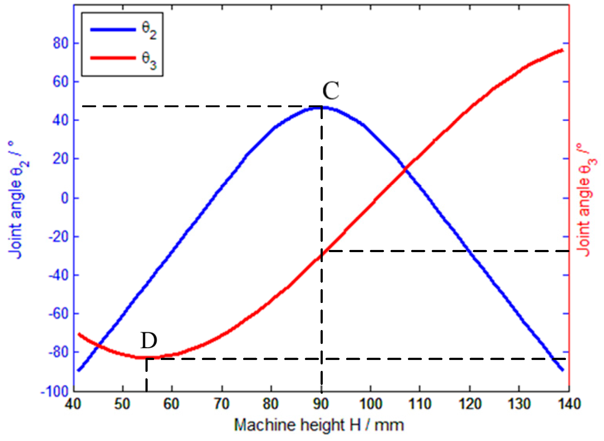
When ${\alpha =30}^{°}$, it can be seen from Figure 10, Figure 11 and Figure 12 that point C had the lowest energy consumption, and the low energy consumption static posture of the hexapod robot was

$$\mathrm{H}=90.0\left[\mathrm{mm}\right]{,\theta }_1{=30}^{°}{,\theta }_2={45.4}^{°}{,\theta }_3=-{135.4}^{°}.$$

It can be seen from the simulation results that under the condition of considering the energy consumption target, the total output torque of the joint in the static posture was the smallest. Moreover, the static energy obtained by the method was comprehensively considered under the condition of energy consumption and maximum step size. Since the solution obtained by considering the energy consumption and the maximum step size target was the equilibrium solution, the total output torque was low. This thus verified the correctness of the proposed method.

The same method could be used to obtain low-energy static postures of the robot under different values, as shown in

Table 5. Low-energy static postures of robot under different values of $\alpha$.

$\mathit{\alpha }$	${\mathsf{\theta }}_{\mathbf{i}}\left(\mathit{i}=1,2,3\right)$$[°]$	$\mathbf{H}$ [mm]	$\mathit{M}$$\left[\mathit{N}.\mathit{m}\right]$	$\mathit{R}$ [mm]
0°	${\theta }_1{=0}^{°}$ ${\theta }_2={45.0}^{°}$ ${\theta }_3=-{156.0}^{°}$	40	0.356	0.2927
30°	${\theta }_1{=30}^{°}$ ${\theta }_2={45.4}^{°}$ ${\theta }_3=-{135.4}^{°}$	90	0.112	0.2927
90°	${\theta }_1{=0}^{°}$ ${\theta }_2={10.4}^{°}$ ${\theta }_3=-{100.4}^{°}$	116	0.125	0.2538

.

6. Low-Energy Posture Experiment with Robot Prototype

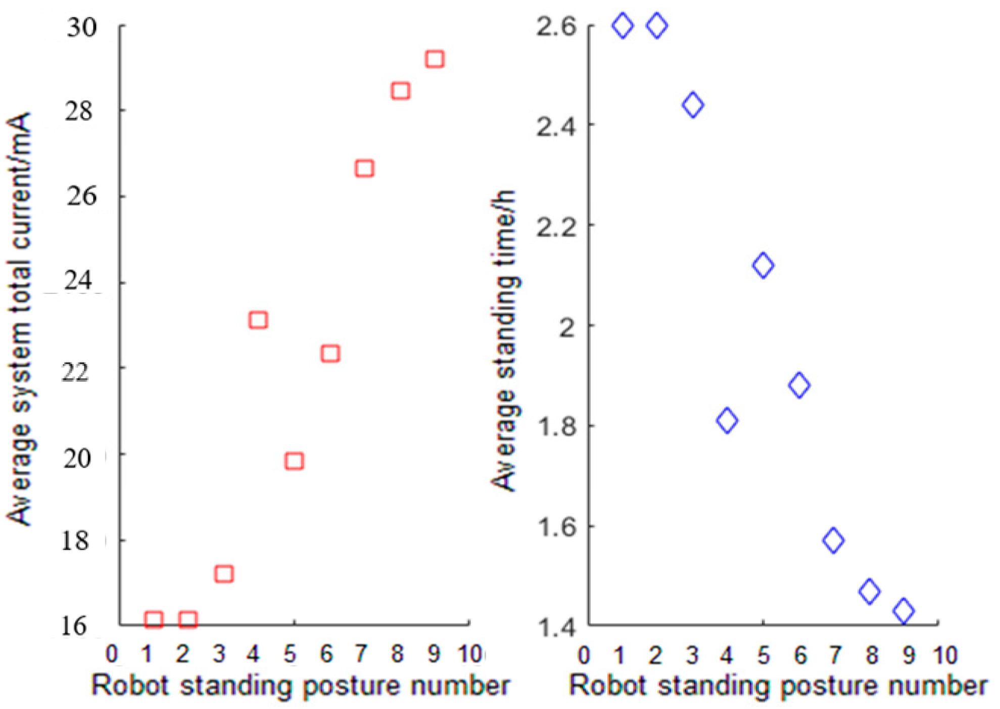
Since the output torque of the servos was proportional to the current,$\mathsf{\tau }\propto I$[27], this paper used the average system total current to measure the static energy consumption of the robot. In the prototype experiment, by directly observing the total current value of the lower computer, the average total current was calculated to compare the relative magnitudes of torque. The magnitude of the current was used to replace the relative magnitude of the torque because there was a positive proportional relationship between them. In this paper, several static postures were selected for two comparative experiments: (1) a prototype test considering only the energy consumption target; and (2) a prototype test considering energy consumption and maximum step targets.

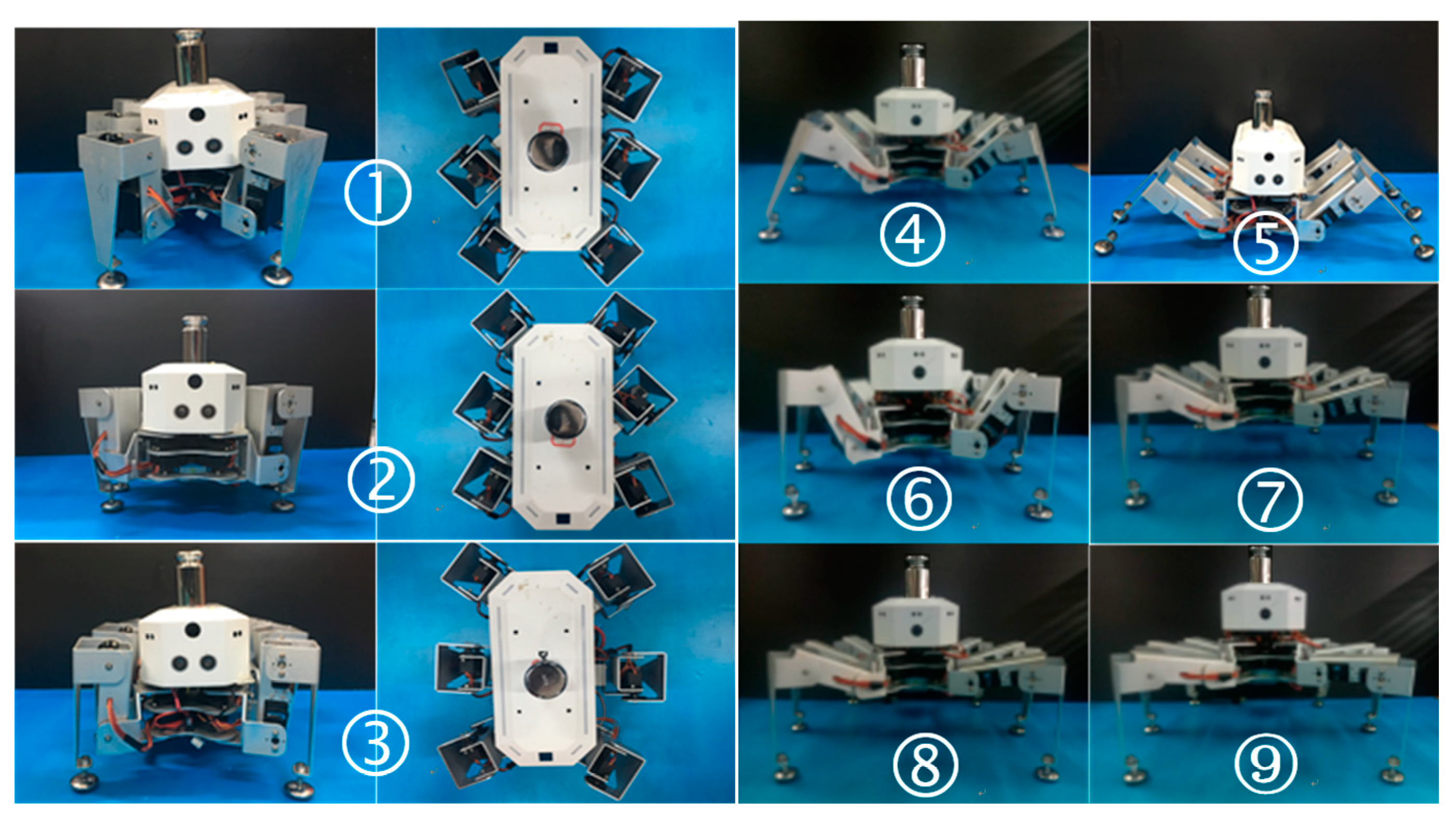
In the first set of prototype experiments, nine typical standing postures were selected as shown in Figure 13. Among them, postures ① and ② were low-energy standing postures obtained in Section 4; posture ③ was a low-energy posture when the joint angle ${\theta }_1$ was$0^{°}$; posture ④ had the same center of gravity height as posture 3; and postures ⑤–⑨ were the static postures when the total weight of the joint output was minimum when the center of gravity height was 30$\mathrm{mm}$, 50$\mathrm{mm}$, 80$\mathrm{mm}$, 110$\mathrm{mm}$, and 140$\mathrm{mm}$, respectively. The experimental results are shown in

Table 6. Data of Figure 14.

Robot Standing Posture Number	Average System Total Torque [N.m]	Average Standing Time [h]
1	16	2.6
2	16	2.6
3	17.8	2.45
4	23.2	1.8
5	19.75	2.15
6	22.55	1.86
7	26.6	1.58
8	28.65	1.47
9	29.5	1.41

and Figure 14.

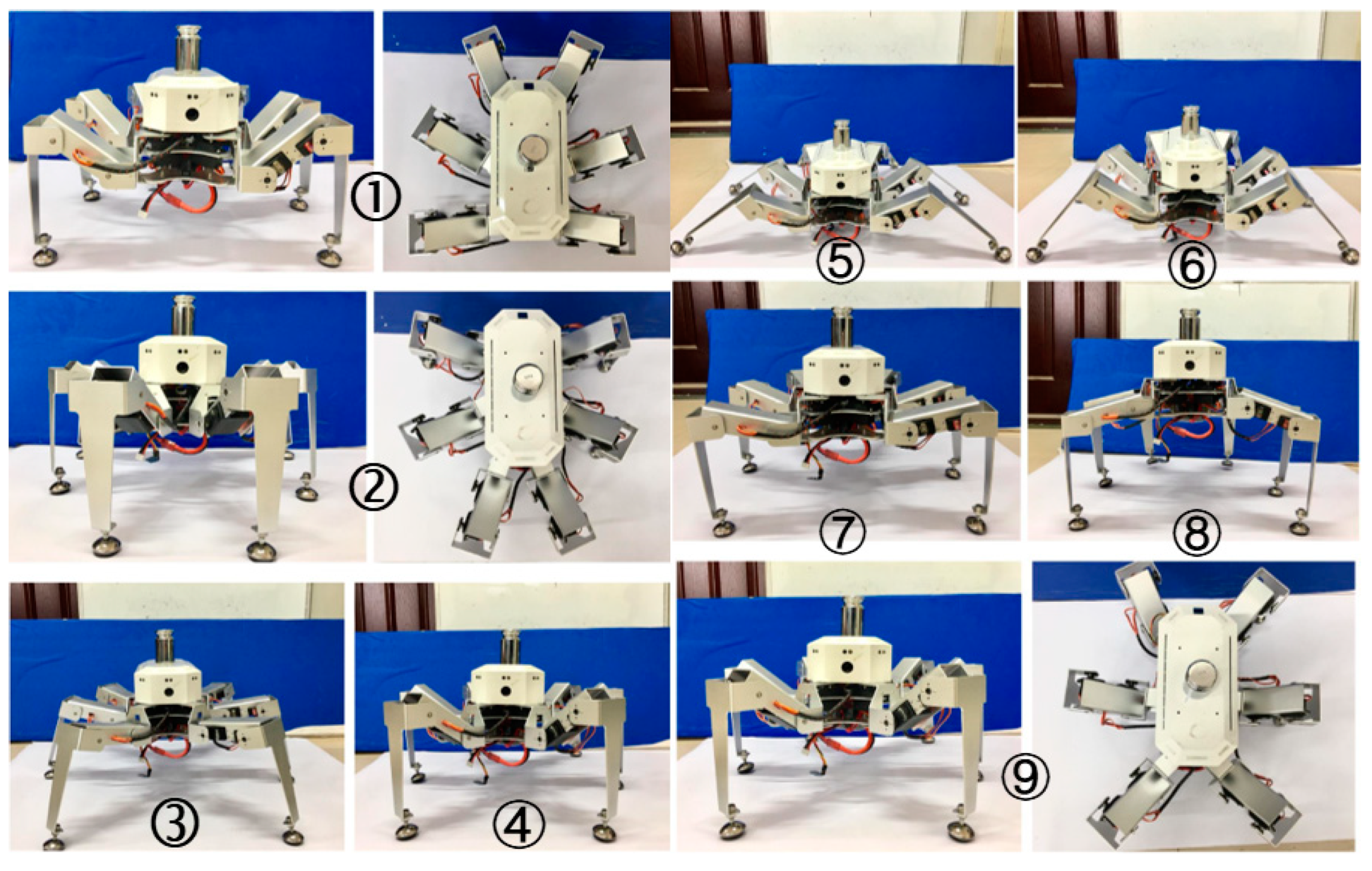
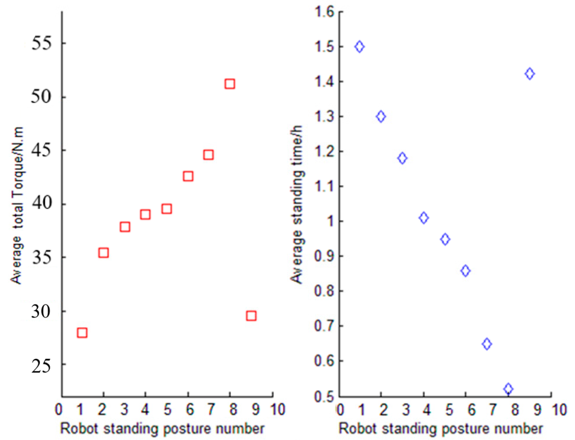
The second set of prototype experiments is shown in Figure 15, where postures ① and ② were low-energy static postures obtained in Section 5; posture ③ had the same center of gravity height as postures ① and ②; posture ④ was in the same position as postures ① and ②; postures ⑤−⑧ were the static postures when the total weight of the joint output was minimum when the center of gravity height was 30$\mathrm{mm}$, 50$\mathrm{mm}$, 80$\mathrm{mm}$, 110$\mathrm{mm}$, 140$\mathrm{mm}$, respectively; and posture ⑨ was a low-energy static posture obtained when $\alpha =0°$. The experimental results are shown in

Table 7. Data of Figure 16.

Robot Standing Posture Number	Average System Total Torque [N.m]	Average Standing Time [h]
1	28	1.5
2	35.4	1.3
3	37.8	1.18
4	39	1.01
5	39.5	0.95
6	42.55	0.86
7	44.6	0.65
8	51.2	0.52
9	29.5	1.42

and Figure 16.

The experiment showed that the energy consumption of the static posture obtained in this paper was the lowest when only the energy consumption target was considered. When considering the energy consumption and the maximum step target, the static posture obtained by the method proposed in this study had the lowest energy consumption under the premise of ensuring the flexibility of the motion state. Therefore, the correctness and validity of the proposed method were verified.

7. Conclusions

In this paper, a hexapod robot with low-speed motion and the relationship between postures and energy consumption were studied. Through theoretical analysis and experimental research, the following conclusions are drawn.

(1) An analysis method for low-energy postures in the static state was proposed. The research showed that there was a clear correspondence between robot postures and energy consumption. The method could be applied to a multi-legged robot, and the static energy posture was adjusted to reduce the energy consumption of the robot in a non-moving state.

(2) The low-energy postures in the static state were obtained by the proposed energy consumption model, and the trajectory design was established by comprehensively considering the motion characteristics of the robot from the static state to the motion state. Using the maximum step size target, by obtaining the postures constraint equation, the constraints of increasing the postures of the robot further restricted the movable range of the joints of the robot legs, thereby obtaining an effective low-energy posture.

(3) A robot model was established, and an experimental prototype was developed. The static postures were solved by the proposed method. The effectiveness of the method was verified by simulations and experiments with the physical prototype. Experiments showed that the proposed method could achieve the goal of reducing energy consumption and increasing endurance time while ensuring the flexibility of the robot.

(4) The focus of this paper was to discuss the relationship between energy consumption and the orientation of the legged robot. From the point of view of bionics, the influence of the change of posture on the overall energy consumption in the static state was obvious. The specific measurement of the overall energy consumption needed to consider a number of influencing factors. The use of torque as a consideration in this paper was to simplify the problem and to highlight the research focus and objectives. We wish that the trends of robot attitude change and energy consumption change could be obtained through the method proposed in the paper, in order to further study in future the method of active attitude control to reduce the overall energy consumption of the robot.

(5) Although the robot with low speed movement was taken as the research object, the establishment of the energy model of the foot robot has a similar analysis process. The output torque of the joints of the legs can be obtained through the static analysis of the legs, so that the energy consumption of the whole robot can be analyzed. Therefore, the method proposed in this paper was general for legged robots, especially for bionic insect legged robots. Secondly, considering the flexibility of the robot, the introduction of the maximum step performance index, and the equalization method based on energy consumption and maximum step size, this method was also applicable to any foot robot. In the experimental part of the article, although a specific robot platform was selected for testing, the variation rule of the whole energy consumption was solved, which was not a specific numerical change, which simplifies the problem and highlights the research methods and objectives.

Future work:

(1) Increase the analysis of robot flexibility. Flexibility is an important indicator of the robot’s motion performance, reflecting the dexterity of the robot’s position in the workspace. Therefore, the next step is to introduce flexibility to replace the maximum step size, optimize the flexibility of the body, and ensure the lowest overall energy consumption of the body at the same time.

(2) In this paper, only the low-energy static postures of the robot in a structured environment were studied. In practical work, robots are used in complex and unstructured environments (the legs of each support leg are not in the same plane). Therefore, the research environment can be extended from a structured terrain to complex unstructured terrain, and the low-energy static postures of the foot robot in different environments can be fully studied. However, the six legs are symmetrically distributed. Due to the influence of terrain and other factors, it is difficult to achieve symmetric distribution of the six legs when the robot is standing still. Therefore, the relationship between the different leg configuration modes and the low-energy static posture of the robot should be studied.