Electromagnetic Testing of Rod Cluster Control Assemblies in Pressured-Water Reactor Power Plants

Abstract

This paper presents an electromagnetic testing system for rod cluster control assemblies used in pressurized-water reactors. The system uses several encircling-type magnetic cameras equivalent to a number of the control rods; each sensor probe composes of an encircling Hall sensor array (EHaS) and a bobbin coil. The EHaS has 16 Hall sensor elements that measure the electromagnetic field distribution in the radial direction of the control rod induced by the bobbin coil for defects. Experiments are performed on artificial defects on the cladding tube of real control rods to simulate short-circumferential grooves (SCGs), sliding wears (SWs), and circumferential cracks (CCs). The system can inspect the artificial SCGs, SWs, and CCs with depths up to 20%, 30%, and 40% of the cladding tube thickness (0.47 mm), respectively. Furthermore, the shape and depth of the defects could be estimated. The standard deviations of depth estimation are 18%, 5.8%, and 6.0% for CCs, SCGs, and SWs. The SCGs and SWs have a small and similar estimation error, but the CCs have the highest error of estimation, and have a small width of 0.2 mm.

1. Introduction

Rod cluster control assemblies (RCCAs) are used in pressurized-water reactors (PWRs) to control fast reactivity changes and stop the reactor when an accident happens. The RCCA usually consists of 16 (14×14 type), 20 (16×16 type), or 24 (17×17 type) control rods. Each control rod includes an absorber consisting of Ag (80%)-In (15%)-Cd (5%) in the core and covered with a cladding tube made of stainless steel (STS340) to prevent corrosion and cracking [1]. Each RCCA is moved upward and downward in the reactor core by a control rod drive mechanism. There are eight guide cards located at the upper side of the reactor core to support the RCCA, which are visible after the nuclear fuel is withdrawn during operation of the nuclear reactor. During operation, wear can occur on the cladding tube due to the up/down movement of the RCCA and vibration of control rods against the guide cards, the vibration of the guide cards themselves, and vibration against the inner walls of the guide tubes on the fuel assemblies [1,2]. The swelling of the absorber can lead to an increase in diameter and result in the appearance of a crack in the cladding tube [1,2]. Additionally, irradiation assisted stress corrosion cracking usually occurs in the cladding tubes and end tips of the control rods [3]. Therefore, it is necessary to inspect and evaluate the defects to ensure the safety and integrity of the PWRs.

Several nondestructive testing systems have been developed and applied for inspection of control rods such as encircling bobbin probes [3,4,5] and multi-array pancake coil probe systems [6]. The encircling bobbin probes use an absolute- or differential-type bobbin coil as a sensor for measuring the rate changes of the total magnetic flux due to the presence of a defect on the control rod. Thus, the spatial resolution is just one circumferential circle, which is low. The encircling bobbin probes are also limited to detecting circumferential cracks [3,4]. The multi-array pancake coil probes use multiple pancake coils arrayed in a probe for improvement of spatial resolution in the circumferential direction. However, the multi-array pancake coil probes still have low spatial resolution due to the large size of the pancake coils. For instance, a probe consisting of an 8×1 pancake coil array has been developed [6]. In addition to this, the sensing coil measures the rate of change of magnetic flux over time. The excitation source is a sinusoidal wave which produces the sinusoidal magnetic flux by the exciting coil. According to Faraday’s law, the output of the sensing coil is a voltage which is proportional to the rate of the magnetic flux over time. In addition, the output voltage is proportional to the frequency of excitation. Thus, the output voltage is low (low sensitivity) at a low frequency of excitation. Therefore, the previous systems are limited in their detectability and quantitative evaluation of defect sizes. Recently, magnetic sensors have been used for directly sensing the magnetic field due to the presence of defects. Numerous Hall sensor and Giant magnetoresistance (GMR) sensor elements are arrayed in the circumferential direction of the probes for inspection of defects at the inner or outer surface of tubes [7,8,9,10,11]. The developed system has efficient inspection capabilities and enables quantitative evaluation of defects.

In this paper, we propose an integrated system comprising 24 encircling Hall sensor array (EHaS) probes that enable the inspection of a 17×17 type RCCA in a single scan. Each EHaS has 16 Hall sensor elements arrayed around an 11.2 mm cylindrical supporter at an interval of 22.5° (2.2 mm). The experiment was performed on real RCCA control rods composed of an AgInCd absorber and a STS304 cladding tube. Artificial short-circumferential grooves (SCGs), sliding wears (SWs), full-circumferential cracks (FCCs), and partial-circumferential cracks (PCCs) on the cladding tubes were tested for verification of the proposed system. Not only the detection of defects but also the potential for the quantitative evaluation of the defects will be discussed.

2. Principle

Figure 1 shows the basic principle of the EHaS probe inserted outside of the control rod with a defect. The EHaS probe consists of a bobbin coil wound around an EHaS. The bobbin coil is an electromagnetic source which is supplied by an AC. An induced current in the circumferential direction of the control rod appears due to the first magnetic field from the coil, and is perturbed by the defect. The intensity of the induced current penetrates the control rod according to the skin effect, with a skin depth calculated by Equation (1) [9,10]. The skin effect limits the penetration depth of the induced current, thus the EHaS probe is sensitive to surface defects. A secondary magnetic field appears due to the induced current, and the radial component (Br) is then measured by the EHaS. By measuring the radial magnetic field Br, the defect can be detected and evaluated quantitatively.

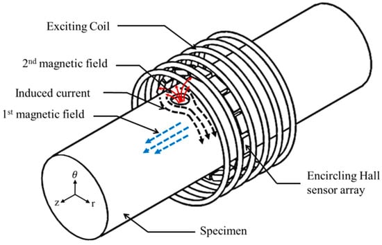
Figure 1. Principle of an Encircling Hall sensor (EHaS) probe.

The output voltages Vr of the EHaS, which have a linear relationship with the magnetic field Br, are processed through high-pass filters (HPFs), amplifiers, root-mean-square (RMS) circuits, and transferred (V_RMS) to a computer by a National Instruments data acquisition (NI-6255 USB type, National Instruments, Austin, Texas, USA). The processing of the signal is simplified as the NI device is also used to control the power supplies for all of the signal processing units and EHaS probe, and to control the scanning of the control rods.

$$\delta =\frac{1}{\sqrt{\pi f\mu \sigma }}$$

(1)

$$V_r\left(t\right)=K·I·B_r\left(t\right)=K·I·B_{r0}·\sin \left(2\pi f·t+\phi \right)$$

(2)

$$V_{RMS}=\sqrt{\frac{1}{T}\underset{0}{\overset{T}{{\displaystyle \int }}}{\left[V_r\left(t\right)\right]}^{2}dt}=\frac{K·I·B_{r0}}{\sqrt{2}}$$

(3)

Here, f, μ, and σ are the exciting frequency, absolute permeability, and electrical conductivity, respectively, of the control rod material, and $K$, $I$, $t$, $B_{r0}$, $T$ and $\phi$ are the Hall constant, the input current of the Hall sensor, and the time, amplitude, period, and phase of the radial magnetic field Br, respectively.

3. Experimental Setup

3.1. Specimens

Figure 2a shows the position of the control rods of a 17×17 type RCCA used in the laboratory test. The 17×17 type RCCA has 24 control rods assembled in a bundle. Each control rod has a diameter of 9.68 mm, cladding tube (STS304) having a thickness (W.T) of 0.47 mm, and an absorber inside made of Ag (80%)-In (15%)-Cd (5%). An inspection stage for the RCCA is shown in Figure 2b, which has 24 holes aligned with the center of the control rods. The holes were positioned in four groups A, B, C, and D, and the group was rotated 90° from each other, as described in Figure 2c. An EHaS probe was assembled at each hole for inspection of a single control rod. Thus, all the control rods in the RCCA could be inspected in just one scan.

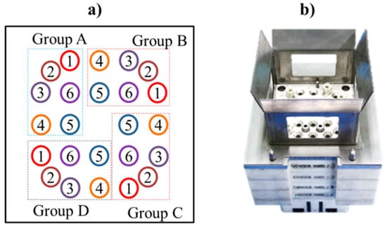
Figure 2. Position of the control rods of a 17×17 type rod cluster control assembly (RCCA) (a), and inspection stage (b).

During operation, there exist several essential phenomena, such as wear and absorber swelling, which influence the lifetime of the control rod. Wear on the cladding of the control rod occurs due to the vibration of the control rods and the axial movement of the RCCA against the guide cards, the vibration of the guide cards themselves, and vibration against the inner walls of the guide tubes on the fuel assemblies [1,2]. Artificial SCGs and SWs were produced for the simulation of wear on the control rod. The swelling of the absorber can lead to an increase in diameter and result in the appearance of a crack in the cladding tube [1,2], which is stimulated by the artificial FCCs and PCCs. The detailed sizes of the SCGs, SWs, FCCs, and PCCs are shown in Table 1, and the shapes in Figure 3. The SCGs have various depths ranging from 20% to 70% of W.T, widths of 10 mm, and are covered 360° around the control rod. The SWs have depths from 30% to 100% of W.T and widths of 50 mm. The circumferential cracks (CCs) have depths from 10% to 60% of W.T, lengths of 45° to 360° in the circumferential direction, and widths of 0.2 mm.

Table 1. Shapes and sizes of the artificial defect (unit: mm, degree; W.T = wall thickness (0.47 mm)).

Type	No.	Depth	%W.T	Degree	Width	Type	No.	Depth	%W.T	Degree	Width
Short-circumferential grooves (SCGs)	# 1	0.047	10	360°	10	Full-circumferential cracks (FCCs)	# 1	0.047	10	360°	0.2
	# 2	0.117	25				# 2	0.094	20
	# 3	0.188	40				# 3	0.141	30
	# 4	0.235	50				# 4	0.188	40
	# 5	0.282	60				# 5	0.235	50
	# 6	0.329	70				# 6	0.282	60
Sliding wears (SWs)	# 1	0.141	30	-	50		#7	0.329	70
	# 2	0.235	50	-		Partial-circumferential Cracks (PCCs)	# 1	0.094	20	45°	0.2
	# 3	0.47	100	-			# 2	0.188	40	90°
	# 4	0.141	30	-			# 3	0.188	40	90°
	# 5	0.235	50	-			# 4	0.188	40	180°
	# 6	0.47	100	-			# 5	0.188	40	270°

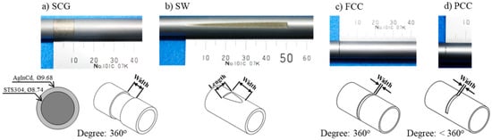
Figure 3. Different artificial defects on the control rods: (a) Short-circumferential groove (SCG), (b) sliding wear (SW), (c) full-circumferential cracks (FCC), and (d) partial-circumferential cracks (PCC).

3.2. Sensor and System Prototype

According to the diameter of the control rods, EHaS probes were designed with an inner diameter of 10.2 mm and an outer diameter of 22.0 mm. Each EHaS probe has 16 Hall sensor elements arrayed around an 11.2 mm cylindrical supporter at an interval of 22.5° (2.2 mm). The bobbin coil is placed outside of the EHaS, which has 168 turns, with a width of 13 mm, using a 0.1 mm copper wire. The inner diameter of the bobbin coil is 13.8 mm. The sensor signal cable length is 10 m from the inspection stage to the signal processing units. The prototype of the EHaS probe is shown in Figure 4.

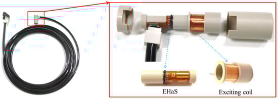
Figure 4. Prototype of an Encircling Hall sensor (EHaS) probe.

For inspection of the entire RCCA, the construction of the EHaS probes, signal processing units, and a prototype of the system is designed as shown in Figure 5. The system is divided into two central units: Unit-1 is mainly for signal processing, and Unit-2 is predominantly for signal acquisition and control. The 24 EHaS probe signal is simultaneously processed by the HPFs (fc = 300 Hz), the 1st stage amplifiers (59.7 dB), and the RMS circuits before arriving at the multiplexer, as shown in Figure 2. The multiplexer extracts the signals from four EHaS probes in the four groups (A, B, C, and D) at the same time. For instance, A-1, B-1, C-1, and D-1 probes operate at the same time. In total, 64 channel signals (4×16) will be outputted at each loop of the multiplexer. The signal is then amplified in the 2nd stage amplifiers (6 dB), digitized by an analog-to-digital converter (NI USB 6255), and stored in a notebook. The software is built based on the LabVIEW program. The 24 EHaS operation takes approximately 72 ms for each data acquisition cycle. For demonstration in this paper, the system is operated at 20 mm/s with a scan step of 1.72 mm and the bobbin coil current is 200 mA–15 kHz.

Figure 5. Block diagram and prototype of the electromagnetic testing system for a 17×17 type RCCA.

4. Experimental Results and Discussions

Figure 6 shows the scan results of the SCGs on a control rod. The offset signal was removed by back data process V_b, as described by Equation (4) and results are displayed in Figure 6a. The signal of each Hall sensor element has a different trend due to the inhomogeneous permeability and conductivity of the specimen, and the variation of lift-off between the sensors and the specimen during the scan. Thus, it is difficult to detect the defects using this processed data. Another approach using the differential signal in the scan direction is described by Equation (5), and the result is shown in Figure 6b. The defect’s signal could be observed clearly, with a high contrast against the background noise. The average signal of all the sensor channels in Figure 6c effectively shows the defect signal and almost the same background noise level in the differential process, but it is a strong trend signal and thus difficult to detect the defects (e.g., #1, 10%). All the SCGs have been detected, and the intensity signal of the defect increases proportionally to the depth.

$$V_b\left(i,j\right)=V_{RMS}\left(i+1,j\right)-V_{RMS}\left(0,j\right)$$

(4)

$$\Delta V_{RMS}\left(i,j\right)=V_{RMS}\left(i+1,j\right)-V_{RMS}\left(i,j\right)$$

(5)

Here, i and j are the scan data index (Z-direction) and sensor element index (θ-direction).

Figure 6. Experimental results of short-circumferential grooves (SCGs) with (a) back data process V_b, (b) differential process ΔV_RMS, and (c) average sensor channels’ signal.

The differential processed signal ΔV_RMS of all the defects is shown in Figure 7. The PCCs from #2–#5 in Figure 7a could be observed but with low intensity compared to the background noise. To better observe a defect, a larger angle is beneficial because of the higher concentration of the electromagnetic field around the defect and, in addition, an increased number of Hall sensor elements enhances the sensitivity. The current EHaS probe had an interval angle of 22°, so it was difficult to detect the 45° angle of the PCC #1. The PCC #5 (270°) was easier to detect than the PCC #4 (180°), PCC #3(90°), and PCC #2(90°). The influence of defect depth could be observed in the signal of the FCCs and SCGs. Small depths such as FCC #1 (10% W.T, 0.047 mm) and #2 (20% W.T, 0.094 mm) could not be detected. FCC #3 and #4 were also difficult to detect, which had depths of 30% W.T (0.141 mm) and 40% W.T (0.188 mm), respectively. FCC #5, #6, and #7 could be observed, which had depths of 50% W.T (0.235 mm). All the SCGs with depths of 10% W.T were detected, and the intensity of the defect increased as the depth increased, as commented in the previous paragraph. The SCGs were much easier to detect than the PCCs and FCCs because their width was much larger (10 mm >> 0.2 mm). With the SW defects, the depth and angle had a relationship with the special shape of the SW: as the depth increased, the angle increased. So, the signal intensity of the SW was significantly increased as the depth increased. An SW with a depth of 50% W.T (0.235 mm, #2, #3, #5, and #6) could be observed, but the small depth (e.g. 30%, 0.141 mm, #1, and #4) was difficult to observe. The large signal inbetween the SW #3 and #4 was from the gap of the absorbers of the control rod.

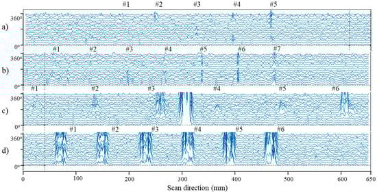
Figure 7. Differential scan signal of the (a) PCCs, (b) FCCs, (c) SWs and (d) SCGs on the control rods.

For improvement of signal quality, the signal from all Hall sensor elements is taken into account in the fusion approach, as described in Figure 8. The square rule of the differential signal is used in the wavelet filter (denoise) and weighted by their average value. The processed signal V_Pro of all the defects is shown in Figure 9. The defect signal was improved so that the 30% depth SW (#1 and #4), 40% depth PCC (#2), and 30% W depth FCC (#3) could be detected. The shapes of the defect were determined as follows: the signal from the SCGs was widely distributed in the axial direction and covers full (or almost) 360°; the signal from the SWs was concentrated in a group, and the signal from the CCs was shortly distributed in the axial direction. The results show that all the SCGs and SWs were detected. However, the small depth CCs could not be observed clearly. For instance, the 30% depth FCC (Figure 9b) looks like a PCC; this could be a variant lift-off during the scan.

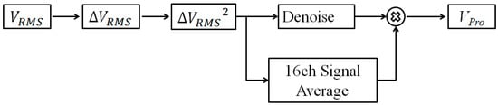
Figure 8. Signal processing diagram.

Figure 9. Denoised and weighted signal V_Pro and of the (a) PCCs, (b) FCCs, (c) SWs and (d) SCGs on the control rods.

For quantitative evaluation of the defect shape and size, two factors are extracted: the amplitude of the signal (h) and the width of the defect signal (WD), as described in Figure 10a. Here, h is the average of all the signal amplitudes in the defect area, which is above the threshold, and WD is the average of all the distances between the first (x₁) and last (x_n) signal, which is above the threshold. h and WD are expressed in Equation (6) and (7), respectively, where, s is the scan step (1.724 mm) and n is the number of data above the threshold. By using the WD, the shape of the defect can be distinguished, as shown in Figure 10b.

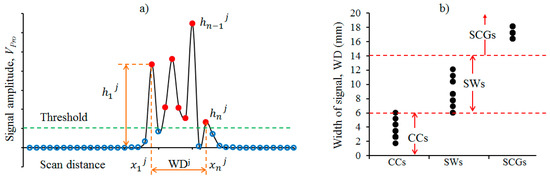
Figure 10. (a) The Hall sensor scan signal of a 10% depth short-circumferential groove and (b) determination of defect shape using the width of the defect signal.

$$h=\frac{1}{16}{\displaystyle \sum }_{j=1}^{16}{\displaystyle \sum }_{i=1}^n{h}_i^j$$

(6)

$$WD=\frac{1}{16}{\displaystyle \sum }_{j=1}^{16}s\left(x_n^j-x_1^j\right)$$

(7)

The relationship between defect signal (log(h)) and defect depth (d) is shown in Figure 11a and is expressed in a linear term in Equation (8). Due to a lack of information, only the depth is taken into account. For the SCGs, SWs, and CCs, the factors (a, b) in Equation (8) are (302.976, 47.1698), (578.4903, 64.5161), and (206.0808, 20.2020), respectively. Then, the depth of the defect was as shown in Figure 11b. The standard deviations of depth estimation are 18%, 5.8%, and 6.0% for the CCs (PCCs + FCCs), SCGs, and SWs. The total estimation of the depth has a standard deviation of 12.1% W.T (0.057 mm). The SCGs and SWs have a small and similar estimation error. The highest error of estimation is for the CCs. This could be the reason that the CCs have a small width of 0.2 mm and the scan step is large at 1.72 mm. It may need to supply more power for the magnetic source to produce a better signal quality of the CCs. The variation of lift-offs, including sensor lift-off and bobbin coil lift-off, is also an important factor that affects the quality of the signal. The current sensor and bobbin coil lift-offs are 0.8 mm and 2.0 mm, which is fine for large defects like the SCGs and SWs but not satisfactory for the small cracks like the PCCs and FCCs, which areonly 0.2 mm in width. Recently, researchers in [12,13] have developed unique algorithms and sensor constructions to compensate the lift-off for the sensing coils. In the future development of the system, it is necessary to minimize the lift-offs and keep less variation during the scan to obtain a higher quality of the signal, especially for the CCs. It is also necessary to develop a method for lift-off compensation using the Hall sensor.

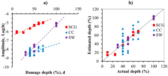
Figure 11. Evaluation of defect depth: (a) relationship between signal amplitude with defect depth and (b) estimation of depth results.

$$d=a\times \log \left(h\right)+b$$

(8)

5. Conclusions

This paper presents an electromagnetic testing system for a 17×17 type rod cluster control assembly (RCCA). The system has 24 sensor probes that enable the inspection of all the control rods in one RCCA. Each sensor probe is composed of 16 Hall sensors arrayed in a circumferential direction and an exciting bobbin coil. Artificial short-circumferential grooves (SCGs), sliding wears (SWs), and circumferential cracks (CCs) on real control rods have been tested to verify the effectiveness of the inspection system. The system was able to inspect the SCGs, SWs, and CCs with the depths of 10%, 30%, and 40% of cladding tube wall thickness (W.T, 0.47 mm), respectively. The shapes the defects could be classified using the width of the defects’ signal. The depth of the defects could be estimated by the average amplitude of the signal. The standard deviations of depth estimation are 18%, 5.8%, and 6.0% for the CCs (PCCs + FCCs), SCGs, and SWs. The total estimation of the depth of all the defects is with a standard deviation of 12.1% W.T (0.057 mm). The SCGs and SWs have a small and similar estimation error, but the CCs have the highest error of estimation and have a small width of 0.2 mm. In future research, more improvement of power for the magnetic source should be taken into account, and it is necessary to minimize the lift-off between the sensor and specimen and the bobbin coil and specimen for obtaining a better quality of the defects’ signal. More different widths and angles of the defects should be considered for a possibility of capturing the relationship with the signal. In addition to this, more advanced signal processing should be carried out for better estimation of the sizes and possibility of shape reconstruction.

References

- Perthuis, S.D. Rcca’s life limitng phenomena: Causes and remedies. In Advances in Control Assembly Materials for Water Reactors, Proceedings of a Technical Committee meeting, Vienna, Austria, 29 November–2 December 1993; IAEA: Vienna, Austria, 1995; pp. 61–78. [Google Scholar]
- Schebitz, F.; Mekmouche, A. Design basic of core components and their realization in the frame of the EPR’s core component development. In Proceeding of the International Youth Nuclear Congress, Interlaken, Switzerland, 20–26 September 2008. [Google Scholar]
- EPRI. Lifetime of PWR Silver-Indium-Cadmium Control Rods; EPRI NP-4512; EPRI: Palo Alto, CA, USA, 1986; pp. 71–75. [Google Scholar]
- Koo, D.S.; Yang, S.Y.; Lee, E.P.; Chun, Y.B.; Lee, J.W. The defect inspection of irradiated fuel rods using different encircling coil probe. In Proceedings of the Korean Nuclear Society Autumn Meeting, Busan, Korea, 27–28 October 2005. [Google Scholar]
- Silvério, F.S., Jr.; Donizete, A.A.J.; Múcio, D.B. The use of eddy current testing for nuclear fuel rods cladding evaluation. In Proceedings of the International Nuclear Atlantic Conference, Santo, Brazil, 20 September–5 October 2007. [Google Scholar]
- Lee, H.J.; Cho, C.H.; Yang, S.H.; Jee, D.H. A study on the nondestructive examination of rod cluster control assembly end tip. In Proceedings of the Korea Nuclear Society Autumn Meeting, Chuncheon, Korea, 25–26 May 2006. [Google Scholar]
- Le, M.; Kim, J.; Vu, H.; Do, H.; Lee, J. Localization and evaluation of corrosion in a small-bore piping system using a bobbin-type magnetic camera. Int. J. Appl. Electromagn. Mech. 2014, 45, 739–745. [Google Scholar] [CrossRef]
- Lee, J.; Jun, J.; Kim, J.; Choi, H.; Le, M. Bobbin-type Solid-state Hall Sensor Array with High Spatial Resolution for Cracks Inspection in Small-Bore Piping Systems. IEEE Trans. Mag. 2012, 48, 3704–3707. [Google Scholar] [CrossRef]
- Le, M.; Lee, J.; Jun, J.; Kim, J. Estimation of sizes of cracks on pipes in nuclear power plants using dipole moment and finite element methods. NDT E Int. 2013, 58, 56–63. [Google Scholar] [CrossRef]
- Le, M.; Lee, J.; Jun, J.; Kim, J. Quantitative evaluation of corrosion in a thin small-bore piping system using bobbin-type magnetic camera. J. Nondestruct. Eval. 2013, 33, 74–81. [Google Scholar] [CrossRef]
- Sim, S.; Le, M.; Kim, J.; Lee, J.; Kim, H.; Do, H.S. Nondestructive inspection of control rods in nuclear power plants using an encircling-type magnetic camera. Int. J. Appl. Electromagn. Mech. 2015. [Google Scholar] [CrossRef]
- Lu, M.; Meng, X.; Yin, W.; Qu, Z.; Wu, F.; Tang, J.; Xu, H.; Huang, R.; Chen, Z.; Zhao, Q.; et al. Thickness measurement of non-magnetic steel plates using a novel planartriple-coil sensor. NDT E Int. 2019, 107, 102148. [Google Scholar] [CrossRef]
- Lu, M.; Yin, L.; Peyton, A.J.; Yin, W. A Novel Compensation Algorithm for Thickness Measurement Immune to Lift-Off Variations Using Eddy Current Method. IEEE Trans. Instrum. Meas. 2016, 65, 2773–2779. [Google Scholar]
© 2019 by the authors. Licensee MDPI, Basel, Switzerland. This article is an open access article distributed under the terms and conditions of the Creative Commons Attribution (CC BY) license (http://creativecommons.org/licenses/by/4.0/).