Article

Locomotion Control of Snake-Like Robot with Rotational Elastic Actuators Utilizing Observer

1
Department of Advanced Machinery Engineering, School of Engineering, Tokyo Denki University, Tokyo 120-8551, Japan
2
Department of Robotics and Mechatronics, School of Science and Technology for Future Life, Tokyo Denki University, Tokyo 120-8551, Japan
*
Authors to whom correspondence should be addressed.
Appl. Sci. 2019, 9(19), 4012; https://doi.org/10.3390/app9194012
Submission received: 23 July 2019 / Revised: 14 September 2019 / Accepted: 20 September 2019 / Published: 25 September 2019
(This article belongs to the Special Issue Bio-Inspired Robotics II)

Abstract

:
The purpose of this paper is designing a head control system capable of adapting to passive side-slipping. The environments in which snake-like robots are expected to be utilized generally have ground surface conditions with nonuniform frictional coefficients. In such conditions, the passive wheels of the snake-like robot have a chance of side-slipping. To locomote the snake-like robot dexterously, a control system which adapts to such side-slipping is desired. There are two key points to realizing such a system: First, a dynamic model capable of representing the passive side-slipping must be formulated. A solution for the first key point is to develop a switching dynamic model for the snake-like robot, which switches depending on the occurrence of the side-slipping, by utilizing a projection method. The second key point is to adapt the control system’s behavior to side-slipping. An idea for such a solution is to include the side-slipping velocity in the weighting matrices. An algorithm to estimate the occurrence of side-slipping and the particular side-slipping link is constructed, to formulate the dynamic model depending on the actual side-slipping situation. The effectiveness of the designed Luenberger observer and the head control system for side-slipping adaptation is verified through numerical simulation.

1. Introduction

A real snake has a simple, string-like figure and can locomote by utilizing the difference between friction in the propulsive direction and that in the normal direction. It can locomote not only on flat land, but also irregular terrains, such as those of deserts, wildlands, and grasslands, by choosing its motion and posture depending on the environment/task. Moreover, it can realize skilled motions, such as swimming, climbing, and squeezing. Overall, a real snake possesses high adaptability, corresponding to the given environments/tasks. A snake-like robot mimics the high level of adaptability of a real snake and is expected to be adaptable to given environments/tasks.
There have been many studies in the literature focused on the locomotion control of snake-like robots. Hirose, a pioneer in the study of snake-like robots, found that the curvature of a snake changes sinusoidally along its body axis. He named this the “Serpenoid Curve” and applied it to trajectory generation for snake-like robots [1]. Endo et al. implemented the propulsive locomotion control of snake-like robots by utilizing the Serpenoid Curve [2]. In studies extending the Serpenoid Curve, Yamada et al. proposed the kinematics to stabilize the head direction during tracking of the robot to the Serpenoid Curve and implemented the kinematics in a robot [3]. Ma et al. implemented a slope climbing control adjusting the amplitude of the Serpenoid Curve by a simulator [4]. In our previous study, we designed a servo control system for tracking to the Serpenoid Curve [5]. Bing et al. implemented smooth walking by adjusting the Central Pattern Generator (CPG) parameters [6]. Dao et al. proposed a head trajectory tracking control method using CPG and the Amplitude Modulation Method (AMM) [7]. Wang et al. implemented locomotion control of a serpentine crawling robot using CPG and a Fuzzy Logic Controller (FLC) [8]. Manzoor et al. implemented motion control of a modular robot using the CPG algorithm [9]. These studies focused on the kinematics and morphology of the snake, but did not address the dynamics involving interactions with the ground.
To consider such dynamics, locomotion control utilizing the difference of friction, like that of a real snake, has been proposed. Izu et al. [10], Yamakita et al. [11], and Matsuno et al. [12] implemented locomotion control avoiding singular configurations, based on dynamic manipulability, by regarding friction in the axial direction as a constraint force. Nakajima et al. realized the locomotion control of a snake-like robot by considering a transition between two nonparallel planes [13]. Fukushima et al. proposed a front-unit tracking control theory utilizing only the current target velocity for the front-unit of a snake-like robot using a screw-driving mechanism [14]. Ariizumi et al. proposed a head position tracking control system, which was capable of locomotion even when a joint suddenly lost energy [15]. In addition, Tanaka et al. implemented a semi-autonomous step climbing control by utilizing both sensor information and a three-dimensional manipulation method [16], and proposed a workspace control system for a redundant robot with a gripper on its head part [17]. They also proposed a shape control method for a snake robot that maintains the head position and orientation as well as avoiding joint limits and self-collision [18], and proposed a smooth controller for an articulated mobile robot with switching constraints [19]. In our previous study, locomotion control of a snake-like robot was realized and a head position control [20,21,22], force control [23], and slope climbing control [24] were designed. Xiao et al. designed a walking method for moving pipes and curved pipes with different diameters and proposed continuous-time dynamical models which integrated an extended Kalman filter (EKF) and an Inertial Measurement Unit (IMU) [25,26]. Bai et al. developed a snake-like robot for coal mine rescue and proposed an algorithm to avoid obstacles using the particle swarm optimization weight coefficient of extreme learning machine (PSOELM) method [27]. Hongyan et al. proposed a real-time obstacle avoidance algorithm based on multiobjective optimization [28]. Suhara et al. proposed an algorithm which runs through a curved pipe that connects straight pipes by spiral rotation [29,30]. Ariizumi et al. analyzed the three actions of sidewinding locomotion, sinus-lifting motion, and lateral undulation of a snake-like robot [31]. Rollinson et al. used an extended Kalman filter (EKF) to move a pipe that cannot be passed by a wheeled robot [32]. Takagi et al. proposed a control design method using side-thrust links, in which the amplitude varies with time [33,34]. Malayjerdi et al. analyzed three-dimensional motion, based on the Gibbs–Appell method [35,36]. These studies have supposed either a uniform or infinite friction coefficient. However, the friction coefficient is generally nonuniform in an actual environment and is finite. Therefore, side-slipping normally occurs, even if the robot features passive wheels.
To address such an issue, control systems based on a dynamic model with side-slipping have also proposed. Bando et al. realized a localization on pipes by sounds during locomotion [37]. Takemori et al. implemented locomotion control over irregular ground, such as a flanged pipe or rubble terrain, by utilizing a dynamic model without considering side-slipping [38,39]. Additionally, Takemori et al. designed a control system to fit configurations of a snake-like robot to targets, by connecting simple shapes, such as straight lines, arc shapes, and spirals [40]. In the work by the authors of [40], ladder climbing locomotion was implemented by the proposed method [40]. For another example, Tanaka et al. proposed a shape-control system for a snake-like robot which preserves the head coordinate [18]. In the work by the authors of [18], the side-slipping was actively controlled by lifting up part of the robot’s body. However, side-slipping occurs unpredictably and is uncontrollable. Thus, it can be regarded as passive for the control system.
The purpose of this study is to design a head position control system which is capable of adapting to passive side-slipping. There are two key points to realize this: First, a dynamic model capable of representing passive side-slipping must be formulated. Second, the control system must be able to adapt to the side-slipping. A solution for the first key point is to switch a dynamic model of the snake-like robot, depending on occurrence of side-slipping. In this paper, the Projection Method [41,42,43] is utilized for this solution. The linear complementarity problem (LCP) is a general method for switching the dynamic model [44]. Likjebäck et al. [45] and Suzuki [46], as well as our previous study, formulated a dynamic model capable of switching model depending on environmental load forces or frictional forces. However, Suzuki noted that there is an issue in real-time processing, due to its heavy calculation load. The Projection Method provides a means to provide a further solution to this issue. The Projection Method is a system modeling method that can be used to derive a dynamic model focusing on constraints of its system, and is capable of formulating constraint forces in parallel with the dynamic model of the system. In addition, the constraint forces can be added to change the dynamics (i.e., is able to switch the dynamic model). Static frictional forces generated in the axial direction of the passive wheel can be regarded as a constraint force in the Projection Method. Therefore, by switching the added constraint forces, depending on the side-slipping, the dynamic model is switched. Based on this idea, the dynamic model of a snake-like robot without constraints, with respect to the side-slipping of the passive wheel, is derived first. Note that the model addressed in this paper has a Rotational Elastic Actuator (REA) installed [47], in order to consider interaction with the environment. Second, the constraint forces in the axial direction are formulated and are added into the dynamic model. A solution for the second key point is to tune the weighting matrices, depending on the side-slipping, in order to converge the side-slipping as soon as possible. An idea for this solution is to include the side-slipping velocity into the weighting matrices. The control system designed in this paper consists of a state observer and a nonlinear quadratic regulator, both based on the State-Dependent Riccati Equation (SDRE) [48,49]. As the state observer, the Luenberger observer is adopted, in order to verify the theoretical effectiveness of our ideas without any noise. To estimate the state accurately, establishing an accurate model is crucially important (i.e., the model must include accurate constraint forces corresponding to the actual side-slipping situation). To accomplish this, an algorithm to estimate the occurrence of side-slipping and the side-slipping link is constructed. The algorithm discriminates both the occurrence of side-slipping and the side-slipping link from the estimated state and observed output. The weighting matrices of the Luenverger observer are tuned depending on the discrimination result. Rapid and accurate state estimation are obtained. Additionally, in the nonlinear quadratic regulator, the discrimination result is utilized to construct an accurate state-space representation. Furthermore, control inputs are obtained by including the velocities in the axial direction into the weighting matrices.
This paper is organized as follows: In Section 2, the dynamic model of a five-link snake-like robot with passive side-slipping switching is derived. The passive side-slipping is represented by utilizing the constraint forces formulated by the Projection Method. Next, the Luenberger observer based on SDRE is designed in Section 3. The algorithm to estimate the generation of side-slipping is also constructed. In Section 4, the head position control system which adapts to the side-slipping is designed. The idea to include the velocities in the axial direction into the weighting matrices of SDRE, which is also proposed in detail. The effectiveness of the designed Luenberger observer and the designed head position control are verified through numerical simulation in Section 5. Section 6 concludes the paper.

2. Modeling of the Snake-Like Robot Switching Side-Slipping Passively

In this section, the dynamic model of a five-link snake-like robot with passive side-slipping is derived. As a modeling method, the Projection Method is utilized. The Projection Method provides a dynamic model of the system, as well as its constraint forces. For the constraint forces, forces to connect the robot’s link and the ones to prevent side-slipping are listed. In this paper, the forces to prevent side-slipping are calculated depending on the environment (i.e., passively) and, by adding them into the model, side-slipping of the model occurs passively. According to this, the dynamic model of the snake-like robot without constraints, with respect to the side-slipping of the passive wheel, is derived first. After that, the constraint forces to prevent side-slipping, which passively switches corresponding to the environment, are derived and the initial model is extended.

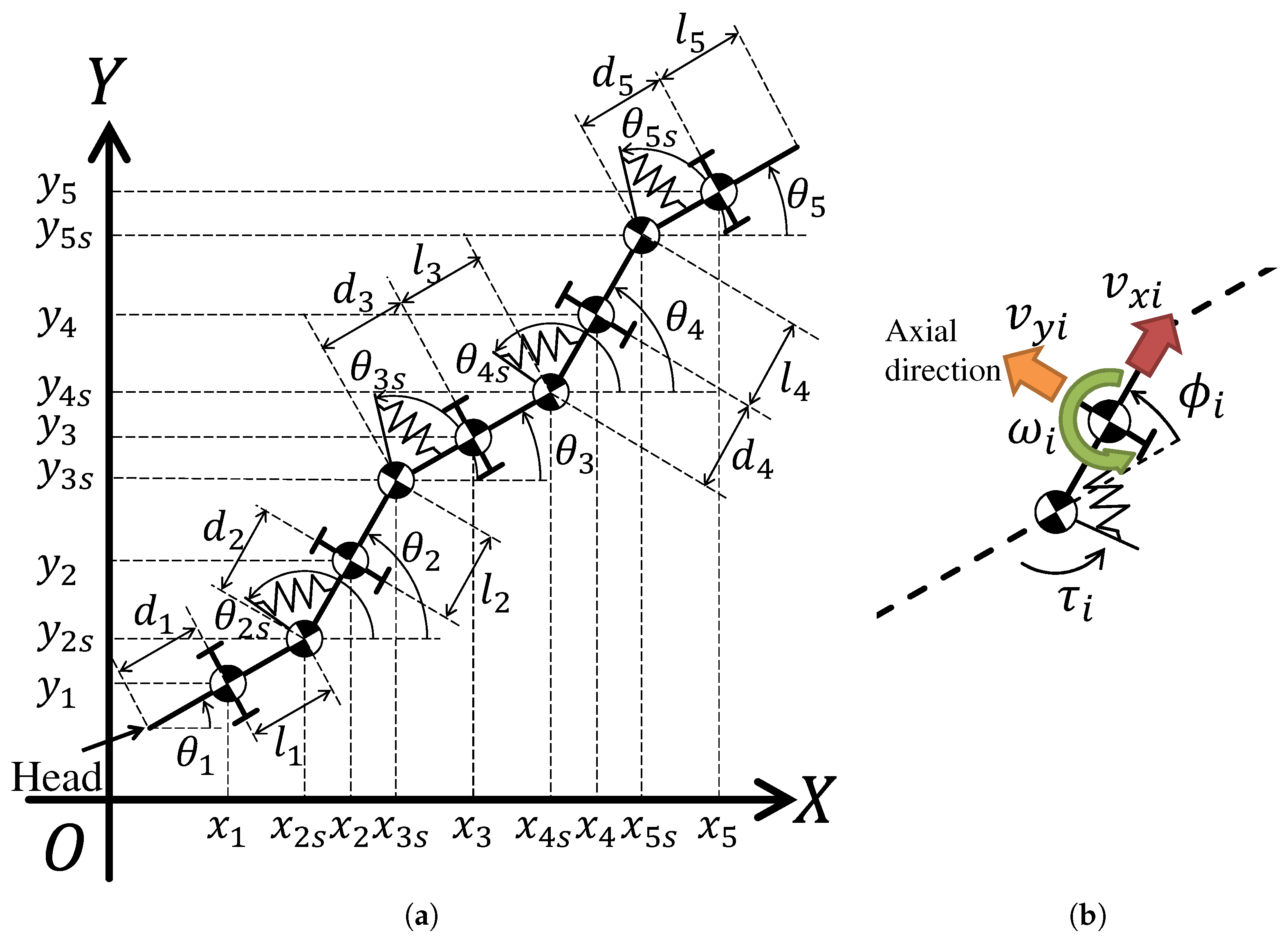
2.1. Modeling of the Five-Link Snake-Like Robot with a Rotational Elastic Actuator

First, a dynamic model of the snake-like robot without a constraint for the passive wheels without side-slipping is derived. A schematic figure of the model is shown in Figure 1, and its physical parameters are defined in Table 1. From Figure 1, the passive wheel is installed at the center of gravity of each link. The subscript s represents the element related to the spring; θ i ( i = 1 , , 5 ) and θ j s ( j = 2 , , 5 ) represent the absolute angle of each link and spring, respectively; ω i , v x i , v y i and ω j s , v x j s , v y j s ( i = 1 , , 5 , j = 2 , , 5 ) represent quasi-velocities at each center of gravity.
First, a model of the constraint-free system is derived. From Figure 1, the generalized coordinate x p of this system is defined as
x p = x p 1 x p 2 s x p 2 x p 5 s x p 5 T , x pi : = θ i x i y i , i = 1 , , 5 , x pjs : = θ j s x j s y j s , j = 2 , , 5 .
As deriving the model of the constraint free system is equivalent to formulating motion equations, both in the rotational direction and in the translation direction of (1) (according to Newton’s equation of motion), the model is derived as follows,
M p x ¨ p = h p ,
where M p and h p represent the generalized mass matrix and the generalized force matrix, respectively, which are defined as follows,
M p = diag ( M p 1 , M p 2 s , M p 2 , , M p 5 s , M p 5 ) , h p = h p 1 h p 2 s h p 2 h p 5 s h p 5 T , M pi : = diag ( J i , m i , m i ) , i = 1 , , 5 , M pjs : = diag ( J j s , m j s , m j s ) , j = 2 , , 5 , h pi : = τ i + 1 k i ( θ i θ i s ) C i ( θ ˙ i θ ˙ i s ) + C i + 1 s ( θ ˙ i + 1 s θ ˙ i ) 0 0 , h pjs : = τ j + k j ( θ j θ j s ) C j ( θ ˙ j s θ ˙ j 1 ) + C j ( θ ˙ j θ ˙ j s ) 0 0 .
τ i ( i = 1 , , 6 ) denotes the input torques into each joint; note that τ 1 = τ 6 = 0 and C 1 = C 6 s = 0 , from Figure 1, at the first and fifth links, have no joint at their front and rear, respectively. Furthermore, from Figure 1b, the quasi-velocity v is defined as follows,
v = v 1 v 2 s v 2 v 5 s v 5 T , v i : = ω i v x i v y i , i = 1 , , 5 , v js : = ω j s v x j s v y j s , j = 2 , , 5 .
From Figure 1, the velocity transformation matrix A relates the generalized coordinate x p and the quasi-velocity v as follows,
A = diag ( A 1 , A 2 s , A 2 , , A 5 s , A 5 ) A i : = 1 0 0 0 cos θ i sin θ i 0 sin θ i cos θ i , i = 1 , , 5 , A js : = 1 0 0 0 cos θ j s sin θ j s 0 sin θ j s cos θ j s , j = 2 , , 5 ,
By Equation (3), Equation (2) is transformed as follows:
M v ˙ = h ,
where, M = A T M p A , h = A T ( h p M p A ˙ v ) .
Second, a constraint matrix C of the system satisfying Cv = 0 is derived. With respect to the positions of the centers of gravity, a holonomic constraint is represented as follows,
Φ h = Φ h 2 s T Φ h 3 T Φ h 5 s T Φ h 5 T T = 0 , Φ hj = x j s x j 1 l j 1 cos θ j 1 y j s y j 1 l j 1 sin θ j 1 , Φ hjs = x j x j 1 s d j 1 cos θ j y j y j 1 s d j 1 sin θ j .
In this paper, the dynamic model without the constraint, in which the passive wheels are not side-slipping, is derived, to design a control system which allows side-slipping. Therefore, the constraint matrix of the system is defined as follows,
C = Φ h x p A .
By utilizing (5), the model satisfying the constraint conditions is derived as follows:
M v ˙ = h + C T λ ,
where λ represents the Lagrange multipliers and denotes the constraint forces of the system in the Projection Method.
Finally, Equation (6) is projected into the tangent speed space and the dynamic model is obtained. From (1), the constraint-free system has 27 DOF. From (4), the system is constrained by 16 holonomic constraints. Therefore, the constrained system has 11 DOF. Now, we set the tangent speed as follows,
q ˙ = ω 1 v x 1 ω 2 s ω 3 s ω 4 s ω 5 s v y 1 v y 2 v y 3 v y 4 v y 5 T .
The tangent speeds are chosen to be suitable for the control system. In this case, ω 1 and v x 1 correspond to the first link, ω j s ( j = 2 , , 5 ) are the motor velocities and v y i ( i = 1 , , 5 ) are velocities in the axial direction. The quasi-velocity is replaced such that v = q ˙ T , v q T T is satisfied, where v q represents the dependent velocities with respect to q ˙ . Furthermore, the constraint matrix C is decomposed into C = C 1 , C 2 , satisfying C v = C 1 q ˙ + C 2 v q = 0 . The complementary orthogonal matrix D satisfying both CD = 0 and v = D q ˙ is derived as follows,
D = I 11 × 11 C 2 1 C 1 ,
where I m × n represents the m × n identity matrix. Then, Equation (6) is projected into the tangent speed space by the derived complementary orthogonal matrix D , and we obtain the dynamic model of the five-link snake-like robot as follows,
D T MD q ¨ + D T M D ˙ q ˙ = D T h .

2.2. Constraint Forces to Prevent Side-Slipping

In this section, the constraint forces to prevent side-slipping of the passive wheels of the snake-like robot are derived. Suzuki utilized the Linear Complementarity Problem (LCP) [44] to formulate these. However, they also noted that there was an issue of high computation times preventing efficient real-time control [46]. To overcome this issue in this paper, the constraint forces to prevent passive wheel side-slipping are formulated by extending the constraint matrix derived using the Projection Method. First, the constraint matrix is extended. Second, using the extended constraint matrix, the constraint forces to prevent side-slipping are formulated. Finally, by utilizing the formulated constraint forces, Equation (7) is extended.
First, the constraint matrix of the system is extended. As shown in Figure 1, let the constraint force in the axial direction and maximum static frictional force of i-th link be denoted by f n i and f m a x , respectively. In the axial direction of the passive wheel of a snake-like robot, the constraint forces preventing side-slipping from occurring satisfy the following condition,
v y i = 0 f n i f m a x , ( i = 1 , , 5 ) .
In the above equation, as v y i = 0 , ( i = 1 , , 5 ) can be described as non-holonomic constraints, we define the following new constraint matrix,
C n = C n 1 T C n 2 T C n 3 T C n 4 T C n 5 T T , C ni = v y i v , ( v y i = 0 f n i f m a x ) , , ( others ) , ( i = 1 , , 5 ) .
Moreover, both the constraint matrix of the system and the Lagrange multipliers, as the constraint forces of the system are extended as C = C T C n T T and λ = λ T λ n T T , respectively; note that λ n represents the constraint force to prevent side-slipping. By utilizing the extended constraint matrix and the Projection method, the extended constraint force λ , including the constraint forces to prevent side-slipping λ n , is formulated as follows,
λ = ( C M 1 C T ) 1 C ( D ˙ q ˙ M 1 h ) .
Finally, by utilizing the formulated constraint force in the axial direction, Equation (7) is extended. The motion (6) in the quasi-velocity coordinate is extended, as follows:
M v ˙ = h + C λ .
Note that (8) is equivalent to the dynamics model of the snake-like robot without side-slipping, unless any link is side-slipping. By projecting (8) into the tangent speed space, by utilizing the complementary orthogonal matrix D , we obtain the extended dynamics model shown in (9):
D T MD q ¨ + D T M D ˙ q ˙ = D T h + D T C n T λ n .

3. Design of the Luenberger Observer

In this section, a Luenberger observer is designed based on SDRE. The key functions of the observer designed in this section are to estimate the passive side-slipping occurring and to tune the observer gains to adapt to it. First, the observable states are discussed quantitatively. Second, the Luenberger observer is designed, based on SDRE. Finally, an algorithm for state estimation for adaptive side-slipping determination is constructed, and the tuning algorithm of observer gain, corresponding to the result of the state estimation algorithm, is constructed.
First, the observable states are discussed. As installation of a rotary encoder in each joint and each elastic part was realized in our previous study [47], the related angles of each joint ϕ j ( j = 2 , , 5 ) and twist angles of the springs s j ( j = 2 , , 5 ) are observable. Additionally, as the installation of a camera on the head link has also been realized in related studies [50,51], the absolute angle θ 1 and position ( x 1 , y 1 ) of the robot’s head are observable. On the other hand, velocity sensors are not installed, so as to save cost and energy; thus, the tangent speed is unobservable. From the above discussion, the observable states (i.e., the output of the system) y are
y = y ϕ T s T T = θ 1 x 1 y 1 ϕ 2 ϕ 3 ϕ 4 ϕ 5 s 2 s 3 s 4 s 5 T .
Second, the Luenberger observer is designed, based on SDRE. The generalized force matrix h is resolved as follows,
h = Eu + F θ ˙ + Gs , u = τ 2 τ 3 τ 4 τ 5 T , θ ˙ = θ ˙ 1 θ ˙ 2 s θ ˙ 2 θ ˙ 5 T , s = s 2 s 3 s 4 s 5 T = θ 2 θ 2 s θ 3 θ 3 s θ 4 θ 4 s θ 5 θ 5 s T ,
where
E = h u , F = ( h Eu ) θ ˙ , G = ( h Eu F θ ˙ ) s .
By utilizing the relation v = D q ˙ , the matrices H , H s , and H y satisfying θ ˙ = H q ˙ , s ˙ = H s q ˙ , and y ˙ ϕ = H y q ˙ , respectively, are defined as follows,
H = D ( 1 ) D ( 4 ) D ( 7 ) D ( 10 ) D ( 13 ) D ( 16 ) D ( 19 ) D ( 22 ) D ( 25 ) T , H s = D ( 7 ) D ( 4 ) D ( 13 ) D ( 10 ) D ( 19 ) D ( 16 ) D ( 25 ) D ( 22 ) T , H y = D 1 D ( 7 ) D ( 1 ) D ( 13 ) D ( 7 ) D ( 19 ) D ( 13 ) D ( 25 ) D ( 19 ) T ,
where
D 1 = 1 0 0 0 cos θ 1 sin θ 1 0 sin θ 1 cos θ 1 D ( 1 ) D ( 2 ) D ( 3 ) .
Note that D ( i ) denotes the i-th row vector of the complementary orthogonal matrix D . Furthermore, the constraint matrix of the system is resolved as follows,
λ = α q ˙ + β u + γ s , α = C T ( C M 1 C T ) 1 C ( D ˙ M 1 FH ) , β = C T ( C M 1 C T ) 1 C M 1 E , γ = C T ( C M 1 C T ) 1 C M 1 G .
By defining the output error e and the state of the Luenberger observer x ^ as follows,
e = y y ^ , x ^ = y ϕ T s T q ˙ T T ,
the Luenberger observer is obtained as
x ^ ˙ = A o ( x ^ ) x ^ + B o ( x ^ ) u + L ( x ^ ) T e , y ^ = C o x ^ , A o ( x ^ ) = Z 7 × 7 Z 7 × 4 H y Z 4 × 7 Z 4 × 4 H s Z 11 × 7 K ˜ M ˜ , B o ( x ^ ) = Z 7 × 4 Z 4 × 4 N ˜ , C o = I 11 × 11 Z 11 × 11 ,
where Z m × n represents the zero matrix with m × n ; in addition,
M ˜ = ( D T MD ) 1 D T ( FH M D ˙ + α ) , N ˜ = ( D MD ) 1 D T ( E + β ) , K ˜ = ( D T MD ) 1 D T ( G + γ ) .
Note that an accent mark ∧ represents the estimated state of the observer. Moreover, L ( x ^ ) denotes the observer gain and
L ( x ^ ) = R o ( x ^ ) C o P o ( x ^ ) ,
where P o ( x ^ ) is a symmetric positive definite matrix of following state-dependent Riccati equation,
A o ( x ^ ) P ( x ^ ) + P ( x ^ ) A o ( x ^ ) T + Q o ( x ^ ) P ( x ^ ) C o T R o ( x ^ ) 1 C o P ( x ^ ) = 0 ,
where Q o ( x ^ ) and R o ( x ^ ) represent the weighting matrices for the observer, and are chosen as positive semidefinite and positive definite, respectively.
Finally, the algorithm for adaptive state estimation of side-slipping determination is constructed. The estimation precision of the designed observer depends greatly on the accuracy of the dynamic model; that is, to appropriately extend the dynamic model according to passive side-slipping is a key issue. To extend the model appropriately, slipping links are discriminated by utilizing the estimated state of the observer. Corresponding to the discriminant result, the weighting matrices of the observer are tuned. First, the generation of side-slipping is discriminated. An error vector for it is defined as follows,
e d : = d 1 d 2 d 3 d 4 d 5 T ,
d i = y i θ ^ i x i ( y ^ i θ ^ i x ^ i ) 1 + θ ^ i 2 , ( i = 1 , , 5 ) .
Note that d i represents perpendicular distance from the center of gravity of the i-th link to estimated value of the i-th link. For the error vector, it is expected that, with a decrease in the norm of e d , a corresponding decrease in the error e between observation of output and the estimated state will be observed when the side-slipping link is discriminated appropriately. On the other hand, when side-slipping happens, an increase in the norm of e d and a corresponding increase in the estimation error e are expected, due to difference between the observer model and actual model. Thus, the generation of side-slipping is discriminated when the following condition is satisfied,
e ˙ d [ k ] e ˙ d [ k 1 ] .
When the above condition is satisfied, a link which possesses a maximum value of d i is discriminated as a side-slipping link, and (9) is reformulated. In addition, the weighting matrices of the observer Q o ( x ^ ) and R o ( x ^ ) are tuned, according to the discriminant result of side-slipping:
Q o = diag ( q θ 1 , q x 1 , q y 1 , q ϕ 2 , , q ϕ 5 , q s 2 , , q s 5 , q ω 1 , q v x 1 , q ω 2 s , , q ω 5 s , q v y 1 , , q v y 5 ) , R o = diag ( r 1 , r 2 , r 3 , r 4 ) ,
where
q θ 1 , q x 1 , q y 1 , q ϕ 2 , , q ϕ 5 = 1000 , q s 2 , , q s 5 = 1 , q ω 1 , q v x 1 , q ω 2 s , , q ω 5 s = 1 , 000 , 000 , q v y 1 , , q v y 5 = 1 ( | v ^ y i | 1 . 0 × 10 5 ) , 100 , 000 ( | v ^ y i | > 1 . 0 × 10 5 ) .

4. Design of Head Position Control System Considering Side-Slipping

In this section, the head position control system for a snake-like robot switching the side-slipping passively is designed. A strategy for the control system design is to converge side-slipping immediately. To converge the side-slipping, the weighting matrix of SDRE is tuned corresponding to the side-slipping situation. To design such a control system, a state-space representation including the head position of the snake-like robot is first formulated. Second, the system is reduced, corresponding to the state of side-slipping. Next, the head position control system is designed, based on SDRE. Finally, a tuning algorithm for the weighting matrix to converge the side-slipping is constructed.
First, the state-space representation including the head position of the snake-like robot is formulated. The head position of the snake-like robot ( x h , y h ) is represented as follows,
x h = x 1 d 1 cos θ 1 , y h = y 1 d 1 sin θ 1 .
By utilizing the relation x ˙ p = Av and v = D q ˙ , the velocity of the head position is related with the tangent speed as follows:
x ˙ h y ˙ h = S q ˙ , S = d 1 sin θ 1 1 0 d 1 cos θ 1 0 1 D 1 .
The state vector is set as follows,
x = x h y h s T q T T ,
and the state-space representation including the head position of the snake-like robot is formulated, as (12), by utilizing the estimated state of the observer x ^ :
x ˙ = A ( x ^ ) x + B ( x ^ ) u ,
where
A ( x ^ ) = Z 2 × 2 Z 2 × 4 S Z 4 × 2 Z 4 × 4 H s Z 11 × 2 K ˜ M ˜ , B ( x ^ ) = Z 2 × 4 Z 4 × 4 N ˜ .
Second, the state-space representation is reduced, corresponding to the state of side-slipping. In (12), when no side-slipping link exists, the velocity in the axial direction of its link is uncontrollable, because in a link without side-slipping, it is regarded that there is a constraint with respect to slip prevention (i.e., the velocity in the axial direction is fixed to zero). To avoid uncontrollable links, the state-space representation is appropriately reduced, corresponding to the side-slipping situation. The reduced system is represented as follows,
x ¯ ˙ = A ¯ ( x ^ ) x ¯ + B ¯ ( x ^ ) u .
For example, when all links are slipping,
x ¯ = x = x h y h s T q T T .
For another instance, when no links are side-slipping,
x ¯ = x = x h y h s T ω 1 v x 1 T .
When the first, second, and fourth links are side-slipping,
x ¯ = x = x h y h s T ω 1 v x 1 v y 1 v y 2 v y 4 T .
Next, the head position control system is designed, based on SDRE. Now, we consider a following quadratic cost function for the reduced system:
J = 0 x ^ ¯ T Q ( x ) x ¯ + u T R ( x ^ ) u d t ,
where Q o ( ξ e ) and R o ( ξ e ) are state-dependent weighting matrices, which are chosen to be positive semidefinite and positive definite, respectively. The input u that quasi-minimizes the quadratic cost function is given by utilizing the estimated state of the observer as follows,
u = R ( x ^ ) 1 B ¯ ( x ^ ) T P ( x ^ ) x ¯ ^ ,
where P ( x ^ ) is a symmetric positive definite matrix of the following state-dependent Riccati equation,
A ¯ ( x ^ ) T P ( x ^ ) + P ( x ^ ) A ¯ ( x ^ ) + Q ( x ^ ) P ( x ^ ) B ¯ ( x ^ ) R ( x ^ ) 1 B ¯ ( x ^ ) T P ( x ^ ) = 0 .
Last, the tuning algorithm to immediately converge the side-slipping is constructed. An idea to achieve this is to change the weight for the velocity in the axial direction, with respect to each sampling period. In particular, the velocity in the axial direction is incorporated into the weighting matrix. We set the weighting matrices Q o ( ξ e ) and R o ( ξ e ) as follows,
Q = diag ( Q x h , Q y h , Q s 2 , , Q s 5 , Q ω 1 , Q v x 1 , Q ω j 2 , , Q ω j 5 , Q v y 1 , , Q v y 5 ) , R = diag ( R 1 , R 2 , R 3 , R 4 ) .
where each of the elements are as follows,
Q x h , Q y h = 1 , Q s 2 , , Q s 5 , Q ω 1 , Q v x 1 , Q ω j 2 , , Q ω j 5 = 0 . 1 , R 1 , R 2 , R 3 , R 4 = 0 . 1 .
The elements for the velocity in the axial direction are set, below, according to the idea:
q v y i = 1 + σ [ n ] | v ^ y i | , ( | v ^ y i | > 1 × 10 5 ) , σ [ n ] = k σ [ n 1 ] , σ [ 0 ] = 1000 , k = 1 . 2 .
By setting the elements for the velocity in the axial direction, as above, the weights for both a link which is slipping fast and a link which continues slipping are tuned greater than others. Thus, the control system converges the side-slipping adroitly and locomotes the system effectively.

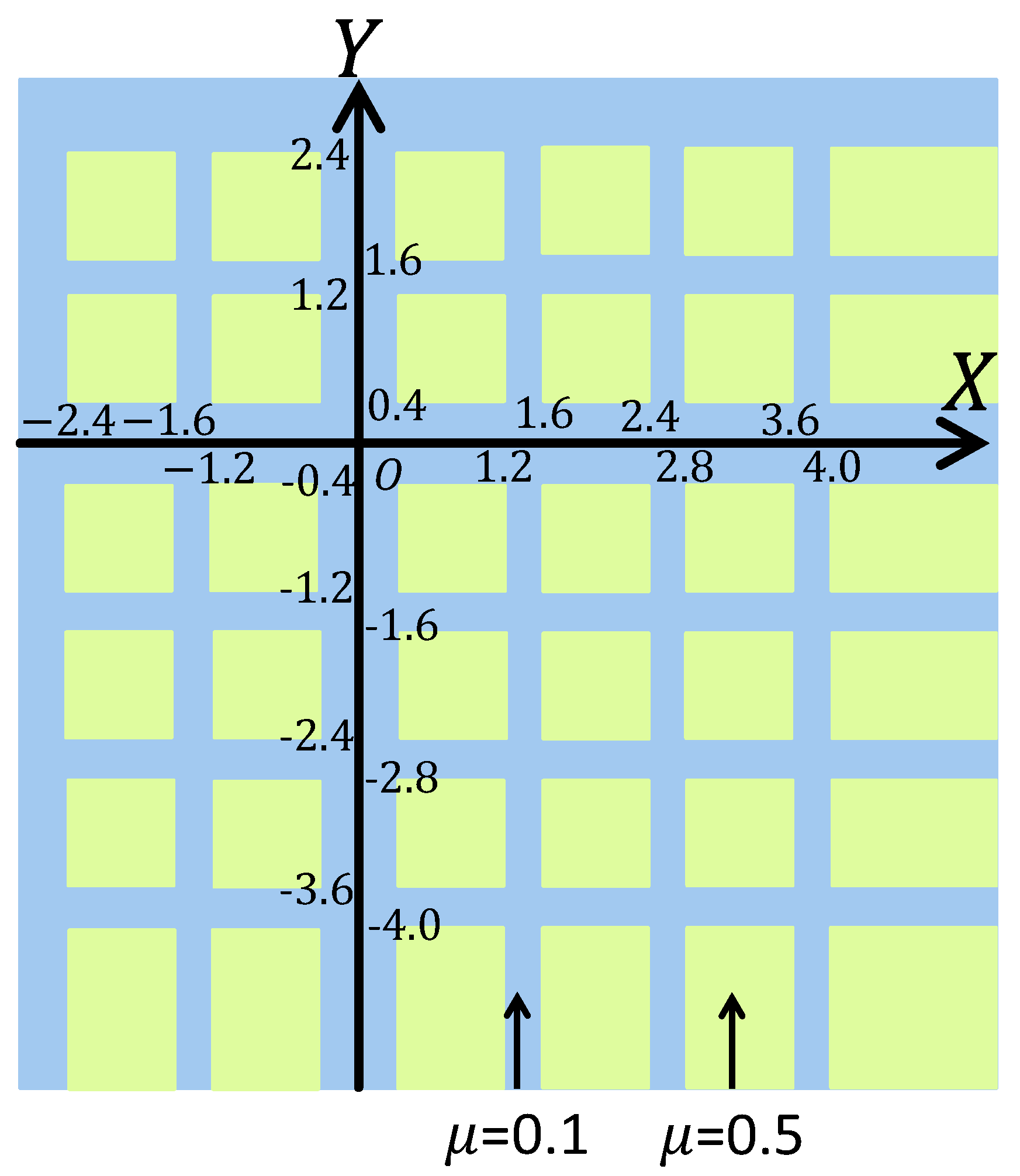
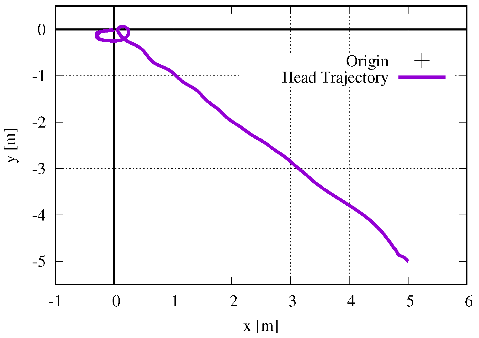
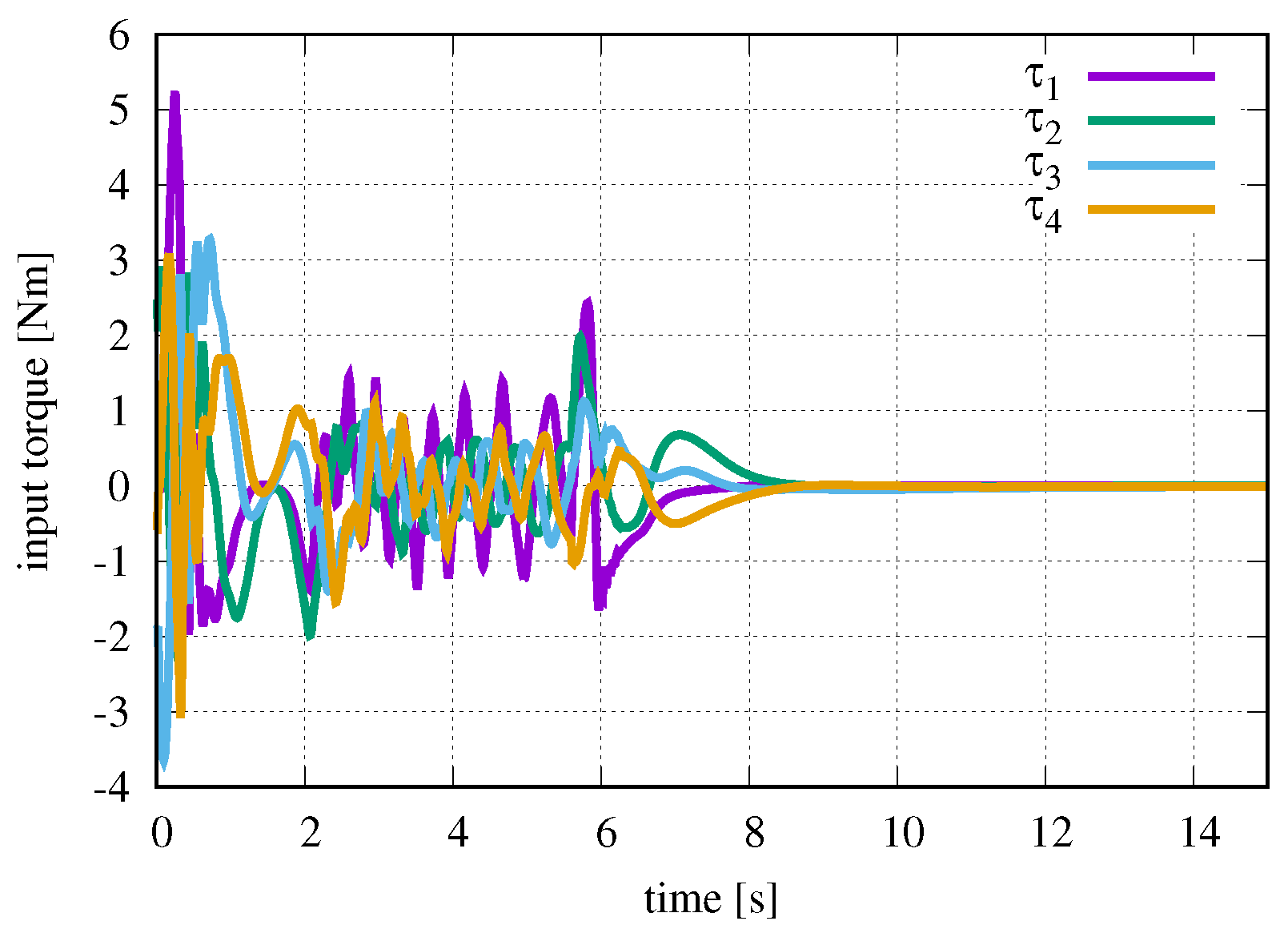
5. Numerical Simulations

The effectiveness of both the designed observer and the designed head position control system were verified through numerical simulations. The numerical simulations were performed by MaTX (Visual C++ 2005 version 5.3.37) [52]. The physical parameters utilized in the numerical simulations are shown in Table 1. The simulation time was 15 s, sampling interval was 0.01 s, and the algorithm used to solve the ordinary differential equation utilized the function “rkf45”. The initial configuration of the robot was θ 1 , θ 3 s , θ 3 , θ 5 s , θ 5 = π / 6 rad and θ 2 s , θ 2 , θ 4 s , θ 4 = π / 6 rad. The static friction coefficient was set as in Figure 2. The set meshed pattern friction coefficients resulted in the generation of side-slipping in an unexpected fashion. The simulations were aimed at verifying adaptability to side-slipping occurring unpredictably, rather than to simulate a practical case. Thus, the simulations were performed in the artificial environment shown in Figure 2. In the simulations, the case studies in three situations, corresponding to different initial positions, were addressed.

5.1. Case 1

In case 1, the initial position of the robot’s head was ( x h , y h ) = (5, −5) m. The simulation results are shown in Figure 3, Figure 4, Figure 5, Figure 6, Figure 7, Figure 8, Figure 9, Figure 10, Figure 11, Figure 12, Figure 13 and Figure 14.
Figure 5, Figure 6 and Figure 7, Figure 11, and Figure 13 clearly show that the designed observer estimated all states accurately and the head position of the robot was controlled by the designed control system even when passive side-slipping occurred, as all states converged. Figure 3 shows that head position control was accomplished, as the head position converged to the origin. From Figure 13, it can be seen, as the constraint forces in the axial direction became greater than the maximum static frictional force at 5.8 s, that side-slipping occurred. However, since side-slipping converged in 0.5 s from the onset of side-slipping, it has been confirmed that the control system considering passive side-slipping functioned appropriately. In addition, Figure 8, Figure 10, Figure 12, and Figure 14 show that the state of the snake-like robot was estimated by the designed observer and the side-slipping link estimation algorithm.

5.2. Case 2

In case 2, the initial position of the robot’s head was ( x h , y h ) = (5, 1) m. The simulation results are shown in Figure 15, Figure 16, Figure 17, Figure 18, Figure 19, Figure 20, Figure 21, Figure 22, Figure 23, Figure 24, Figure 25 and Figure 26.
In case 2, Figure 15, Figure 16, Figure 17, Figure 18, Figure 19, Figure 20, Figure 21, Figure 22, Figure 23, Figure 24, Figure 25 and Figure 26 also show that the designed observer estimated all states accurately, and the head position of the robot was controlled by the designed control system, even when passive side-slipping occurred. In case 2, side-slipping occurred for the first link at 4.6 s, which converged in 0.6 s.

5.3. Case 3

In case 3, the initial position of the robot’s head was ( x h , y h ) = (−1, −2) m. The simulation results are shown in Figure 27, Figure 28, Figure 29, Figure 30, Figure 31, Figure 32, Figure 33, Figure 34, Figure 35, Figure 36, Figure 37 and Figure 38.
In case 3, Figure 27, Figure 28, Figure 29, Figure 30, Figure 31, Figure 32, Figure 33, Figure 34, Figure 35, Figure 36, Figure 37 and Figure 38 also show that the designed observer estimated all states accurately, and that the head position of the robot was controlled by the designed control system, even when passive side-slipping occurred. In case 3, side-slipping occurred for the fifth link at 0.7 s, which converged in 0.4 s.

5.4. Discussion

As a result of the three simulations, we observed the following three facts.
First, the model was switched appropriately by the Luenberger observer. Figure 14, Figure 26, and Figure 38 show that the estimation error of the velocities in the axial direction converged immediately; in particular, “converging the only slipping link” was one of the main characteristics of the designed observer. This means that the designed Luenberger observer worked as expected. Otherwise, the estimated state diverged, or the estimated velocity for other links was non-zero, as the normal Luenberger observer converges the estimation by adjusting all elements impartially. On the other hand, the observer designed in this paper changes its weighting matrices depending on the discrimination result for individual slipping links. This idea gives the observer inequality, and a specific state (i.e., the velocity of the slipping link) was estimated preferentially over others. This characteristic resulted in the simulation results.
Second, the designed control system was able to converge the side-slipping immediately, as was found in Figure 13, Figure 25, and Figure 37. This means that the proposed tuning method worked as expected. Otherwise, the robot continued locomotion with side-slipping longer than that observed in the results. Such a controller might be able to stabilize the system; however, this decreases energy efficiency.
Third, the system generated serpentine locomotion, similar to a real snake. Serpentine locomotion comprises the very basic kinematics of a real snake. Figure 9, Figure 21, and Figure 33 show that the relative angles varied sinusoidally with almost the same phase difference. This is an important characteristic of serpentine locomotion; that is, the control system based on SDRE was able to generate a snake-like morphology without any trajectory generation.

6. Conclusions

In this paper, a head position control system of a snake-like robot capable of adapting to passive side-slipping has been designed. The environments expected for utilizing such snake-like robots are generally ground surfaces featuring nonuniform frictional coefficients. On such surfaces, the passive wheels of the snake-like robot generate side-slipping unpredictably. To locomote the snake-like robot dexterously, a control system which adapts to passive side-slipping was designed. We have regarded the side-slipping which occurs unpredictably to be that which occurs passively, and have proposed the dynamic model. The proposed model represents the presence of (or lack of) side-slipping by passively switching the constraint forces in the axial direction of the passive wheels. The constraint forces in the axial direction were formulated in parallel to the dynamic model of the robot by utilizing the Projection Method. Second, a Luenberger observer to estimate the state of the snake-like robot was designed, based on SDRE. To improve the estimation precision, an algorithm for estimating passive side-slipping was constructed; corresponding to its result, a tuning method for the observer gain was proposed. Next, a head position control system was designed, based on SDRE. In addition, the tuning method to immediately converge the passively generated side-slipping has been proposed. Finally, the effectiveness of the designed observer and the designed head position control system were verified through numerical simulation. The results show that head position control with immediate side-slipping convergence was accomplished, even with unpredictably generated side-slipping.

Author Contributions

Conceptualization, S.N. and M.I.; methodology, S.N.; validation, S.N.; investigation, S.N. and T.Y.; writing—original draft preparation, S.N. and T.Y.; writing—review and editing, S.N. and T.Y.; supervision, M.I. and H.I.; project administration, M.I. and H.I.

Funding

This research received no external funding.

Conflicts of Interest

The authors declare no conflict of interest.

References

  1. Hirose, S. Biologically Inspired Robots: Snake-Like Locomotors and Manipulators; Oxford University Press: Oxford, UK, 1993. [Google Scholar]
  2. Endo, G.; Togawa, K.; Hirose, S. Study on self-contained and terrain adaptive active cord mechanism. J. Robot. Soc. Jpn. 2000, 18, 419–425. [Google Scholar] [CrossRef]
  3. Yamada, H.; Mori, M.; Hirose, S. Stabilization of the head of an undulating snake-like robot. In Proceedings of the 2007 IEEE/RSJ International Conference on Intelligent Robots and Systems, San Diego, CA, USA, 29 October–2 November 2007; pp. 3566–3571. [Google Scholar]
  4. Ma, S.; Tadokoro, N. Analysis of creeping locomotion of a snake-like robot on a slope. Auton. Robots 2006, 20, 15–23. [Google Scholar] [CrossRef]
  5. Nansai, S.; Iwase, M. Tracking control of snake-like robot with rotational elastic actuators. In Proceedings of the 12th International Conference on Control, Automation and Systems, JeJu Island, Korea, 17–21 October 2012; pp. 678–683. [Google Scholar]
  6. Bing, Z.; Cheng, L.; Chen, G.; Röhrbein, F.; Huang, K.; Knoll, A. Towards autonomous locomotion: CPG-based control of smooth 3D slithering gait transition of a snake-like robot. Bioinspir. Biomim. 2017, 12, 035001. [Google Scholar] [CrossRef] [PubMed]
  7. Dao, Q.M.; Vo, Q.T. Design of a CPG-based close-loop direction control system for lateral undulation gait of snake-like robots. In Proceedings of the 2017 International Conference on Advanced Technologies for Communications (ATC), Quy Nhon, Vietnam, 18–20 October 2017; pp. 114–119. [Google Scholar]
  8. Wang, J.; Ouyang, W.; Gao, W.; Ren, Q. Locomotion control of a serpentine crawling robot inspired by central pattern generators. In Proceedings of the Asia-Pacific Signal and Information Processing Association Annual Summit and Conference (APSIPA ASC), Kuala Lumpur, Malaysia, 12–15 December 2017; pp. 414–419. [Google Scholar]
  9. Manzoor, S.; Cho, Y.G.; Choi, Y. Neural oscillator based CPG for various rhythmic motions of modular snake robot with active joints. J. Intell. Robot. Syst. 2019, 94, 641–654. [Google Scholar] [CrossRef]
  10. Izu, H.; Date, H.; Shigeta, K.; Yamanaka, T.; Nakaura, S.; Sampei, M. Locomotion and coiling motion control of snakelike robot using pneumatic actuators. In Proceedings of the 41st SICE Annual Conference—SICE 2002, Osaka, Japan, 5–7 August 2002; Volume 3, pp. 1476–1480. [Google Scholar]
  11. Yamakita, M.; Hashimoto, M.; Yamada, T. Control of locomotion and head configuration of 3D snake robot (SMA). In Proceedings of the IEEE International Conference on Robotics and Automation, ICRA’03. Taipei, Taiwan, 14–19 September 2003; Volume 2, pp. 2055–2060. [Google Scholar]
  12. Matsuno, F.; Sato, H. Trajectory tracking control of snake robots based on dynamic model. In Proceedings of the 2005 IEEE International Conference on Robotics and Automation, Barcelona, Spain, 18–22 April 2005; pp. 3029–3034. [Google Scholar]
  13. Nakajima, M.; Tanaka, M.; Tanaka, K.; Matsuno, F. Motion control of a snake robot moving between two nonparallel planes. Adv. Robot. 2018, 32, 559–573. [Google Scholar] [CrossRef]
  14. Fukushima, H.; Satomura, S.; Kawai, T.; Tanaka, M.; Kamegawa, T.; Matsuno, F. Modeling and control of a snake-like robot using the screw-drive mechanism. IEEE Trans. Robot. 2012, 28, 541–554. [Google Scholar] [CrossRef]
  15. Ariizumi, R.; Takahashi, R.; Tanaka, M.; Asai, T. Head-Trajectory-Tracking Control of a Snake Robot and Its Robustness Under Actuator Failure. IEEE Trans. Control Syst. Technol. 2018. [Google Scholar] [CrossRef]
  16. Tanaka, M.; Nakajima, M.; Suzuki, Y.; Tanaka, K. Development and control of articulated mobile robot for climbing steep stairs. IEEE/ASME Trans. Mechatron. 2018, 23, 531–541. [Google Scholar] [CrossRef]
  17. Tanaka, M.; Tadakuma, K.; Nakajima, M.; Fujita, M. Task-Space Control of Articulated Mobile Robots with a Soft Gripper for Operations. IEEE Trans. Robot. 2018, 35, 135–146. [Google Scholar] [CrossRef]
  18. Tanaka, M.; Tanaka, K. Shape control of a snake robot with joint limit and self-collision avoidance. IEEE Trans. Control Syst. Technol. 2016, 25, 1441–1448. [Google Scholar] [CrossRef]
  19. Tanaka, M.; Nakajima, M.; Tanaka, K. Smooth control of an articulated mobile robot with switching constraints. Adv. Robot. 2016, 30, 29–40. [Google Scholar] [CrossRef]
  20. Watanabe, K.; Iwase, M.; Hatakeyama, S.; Maruyama, T. Control strategy for a snake-like robot based on constraint force and its validation. In Proceedings of the IEEE/ASME International Conference on Advanced Intelligent Mechatronics, Zurich, Switzerland, 4–7 September 2007; pp. 1–6. [Google Scholar]
  21. Watanabe, K.; Iwase, M.; Hatakeyama, S.; Maruyama, T. Control strategy for a snake-like robot based on constraint force and verification by experiment. Adv. Robot. 2009, 23, 907–937. [Google Scholar] [CrossRef]
  22. Yanagida, T.; Kasahara, M.; Iwase, M. Locomotion Control of Snake-like Robot on Geometrically Smooth Surface. IFAC-PapersOnLine 2015, 48, 162–167. [Google Scholar] [CrossRef]
  23. Nansai, S.; Elara, M.R.; Iwase, M. Dynamic Hybrid Position Force Control using Virtual Internal Model to realize a cutting task by a snake-like robot. In Proceedings of the 2016 6th IEEE International Conference on Biomedical Robotics and Biomechatronics (BioRob), Singapore, 26–29 June 2016; pp. 151–156. [Google Scholar]
  24. Tashiro, K.; Nansai, S.; Iwase, M.; Hatakeyama, S. Development of snake-like robot climbing up slope in consideration of constraint force. In Proceedings of the IECON 2012—38th Annual Conference on IEEE Industrial Electronics Society, Montreal, QC, Canada, 25–28 October 2012; pp. 5422–5427. [Google Scholar]
  25. Xiao, S.; Bing, Z.; Huang, K.; Huang, Y. Snake-like robot climbs inside different pipes. In Proceedings of the 2017 IEEE International Conference on Robotics and Biomimetics (ROBIO), Macau, China, 5–8 December 2017; pp. 1232–1239. [Google Scholar]
  26. Bing, Z.; Cheng, L.; Knoll, A.; Zhong, A.; Huang, K.; Zhang, F. Slope angle estimation based on multi-sensor fusion for a snake-like robot. In Proceedings of the 2017 20th International Conference on Information Fusion (Fusion), Xi’an, China, 10–13 July 2017; pp. 1–6. [Google Scholar]
  27. Bai, Y.; Hou, Y. Research of Pose Control Algorithm of Coal Mine Rescue Snake Robot. Math. Probl. Eng. 2018, 2018, 4751245. [Google Scholar] [CrossRef]
  28. Hongyan, L.; Yuanbin, H. A Multi-objective Optimization Behavior Fusion Avoidance Method for Snake-like Rescue Robot. In Proceedings of the MATEC Web of Conferences, Chengdu, China, 16–17 December 2017; Volume 139, p. 155. [Google Scholar]
  29. Suhara, H.; Kamegawa, T.; Gofuku, A. Realization of a snake robot that passes through inside of bent pipe connected with straigt pipes by helical rolling motion. Proc. JSME Annu. Conf. Robot. Mechatron. (Robomec) 2016, 2016. [Google Scholar] [CrossRef]
  30. Kamegawa, T.; Qi, W.; Suhara, H.; Matsuda, E.; Akiyama, T.; Sakai, S.; Takemori, T.; Fujiwara, T.; Matsuno, F.; Suzuki, Y.; et al. Development of a snake robot moving in a pipe with helical rolling motion. Proc. JSME Annu. Conf. Robot. Mechatron. (Robomec) 2017, 2017. [Google Scholar] [CrossRef]
  31. Ariizumi, R.; Matsuno, F. Dynamic analysis of three snake robot gaits. IEEE Trans. Robot. 2017, 33, 1075–1087. [Google Scholar] [CrossRef]
  32. Rollinson, D.; Choset, H. Pipe network locomotion with a snake robot. J. Field Robot. 2016, 33, 322–336. [Google Scholar] [CrossRef]
  33. Takagi, Y.; Sueoka, Y.; Ishikawa, M.; Osuka, K. Analysis and control of a snake-like robot with controllable side-thrust links. In Proceedings of the 2017 11th Asian Control Conference (ASCC), Gold Coast, QLD, Australia, 17–20 December 2017; pp. 754–759. [Google Scholar]
  34. Takagi, Y.; Sueoka, Y.; Ishikawa, M.; Osuka, K. Snake-Like Robot with Controllable Side-Thrust Links: Dynamical Modeling and a Variable Undulation Motion. In Proceedings of the 2018 IEEE/ASME International Conference on Advanced Intelligent Mechatronics (AIM), Auckland, New Zealand, 9–12 July 2018; pp. 63–68. [Google Scholar]
  35. Malayjerdi, M.; Akbarzadeh Tootoonchi, A. Analytical modeling of a 3-D snake robot based on sidewinding. Int. J. Dyn. Control 2018, 6, 1–11. [Google Scholar] [CrossRef]
  36. Malayjerdi, M.; Akbarzadeh, A. Analytical modeling of a 3-D snake robot based on sidewinding locomotion. Int. J. Dyn. Control 2019, 7, 83–93. [Google Scholar] [CrossRef]
  37. Bando, Y.; Suhara, H.; Tanaka, M.; Kamegawa, T.; Itoyama, K.; Yoshii, K.; Matsuno, F.; Okuno, H.G. Sound-based online localization for an in-pipe snake robot. In Proceedings of the 2016 IEEE International Symposium on Safety, Security, and Rescue Robotics (SSRR), Lausanne, Switzerland, 23–27 October 2016; pp. 207–213. [Google Scholar]
  38. Takemori, T.; Tanaka, M.; Matsuno, F. Gait design of a snake robot by connecting simple shapes. In Proceedings of the 2016 IEEE International Symposium on Safety Security, and Rescue Robotics (SSRR), Lausanne, Switzerland, 23–27 October 2016; pp. 189–194. [Google Scholar]
  39. Takemori, T.; Tanaka, M.; Matsuno, F. Gait design for a snake robot by connecting curve segments and experimental demonstration. IEEE Trans. Robot. 2018, 34, 1384–1391. [Google Scholar] [CrossRef]
  40. Takemori, T.; Tanaka, M.; Matsuno, F. Ladder climbing with a snake robot. In Proceedings of the 2018 IEEE/RSJ International Conference on Intelligent Robots and Systems (IROS), Madrid, Spain, 1–5 October 2018; pp. 1–9. [Google Scholar]
  41. Arczewski, K.; Blajer, W. A unified approach to the modelling of holonomic and nonholonomic mechanical systems. Math. Model. Syst. 1996, 2, 157–174. [Google Scholar] [CrossRef]
  42. Blajer, W. A Geometrical Interpretation and Uniform Matrix Formulation of Multibody Systems Dynamics. Z. Angew. Math. Mech. 2004, 81, 247–259. [Google Scholar] [CrossRef]
  43. Ohsaki, H.; Iwase, M.; Hatakeyama, S. A Consideration of Nonlinear System Modeling using the Projection Method. In Proceedings of the SICE Annual Conference, Takamatsu, Japan, 17–20 September 2007; pp. 1915–1920. [Google Scholar]
  44. Cottle, R.W. Linear Complementarity Problem; Springer: Boston, MA, USA, 2009. [Google Scholar]
  45. Liljebäck, P.; Pettersen, K.Y.; Stavdahl, Ø. A snake robot with a contact force measurement system for obstacle-aided locomotion. In Proceedings of the 2010 IEEE International Conference on Robotics and Automation, Anchorage, AK, USA, 3–7 May 2010. [Google Scholar]
  46. Yuta, S. Locomotion Control of Snake-Like Robot Considering Interaction with Environment. Master’s Thesis, Tokyo Denki University, Tokyo, Japan, 2012. [Google Scholar]
  47. Nansai, S.; Suzuki, Y.; Iwase, M.; Izutsu, M.; Hatakeyama, S. Development of snake-like robot with rotational elastic actuators. In Proceedings of the 2011 11th International Conference on Control, Automation and Systems, Gyeonggi-do, Korea, 26–29 October 2011; pp. 19–24. [Google Scholar]
  48. Cloutier, J.R. State-dependent Riccati equation techniques: An overview. In Proceedings of the 1997 American Control Conference (Cat. No. 97CH36041), Albuquerque, NM, USA, 6 June 1997; Volume 2, pp. 932–936. [Google Scholar]
  49. Cimen, T. Survey of state-dependent Riccati equation in nonlinear optimal feedback control synthesis. J. Guid. Control Dyn. 2012, 35, 1025–1047. [Google Scholar] [CrossRef]
  50. Chigisaki, S.; Mori, M.; Yamada, H.; Hirose, S. Design and control of amphibious Snake-like Robot ACM-R5. In Proceedings of the 36th International Symposium on Robotics, Tokyo, Japan, 29 November–1 December 2005. [Google Scholar]
  51. Wright, C.; Buchan, A.; Brown, B.; Geist, J.; Schwerin, M.; Rollinson, D.; Tesch, M.; Choset, H. Design and architecture of the unified modular snake robot. In Proceedings of the 2012 IEEE International Conference on Robotics and Automation, Saint Paul, MN, USA, 14–18 May 2012; pp. 4347–4354. [Google Scholar]
  52. Masanobu, K. MaTX/RtMaTX: A Freeware for Integrated CACSD. In Proceedings of the 1999 IEEE International Symposium on Computer Aided Control System Design (Cat. No. 99TH8404), Kohala Coast, HI, USA, 27 August 1999; pp. 452–456. [Google Scholar]
Figure 1. Schematic figure of a five-link snake-like robot with rotational elastic actuators (REAs). (a) Definition of the generalized coordinate. (b) Definitions of both the quasi-velocity and the relative angle. The springs are installed between links, and are driven by the motor installed on the end edge of the anterior link. The posterior link is driven by the spring. From panel a, τ 1 and τ 6 are nonexistent (i.e., τ 1 = τ 6 = 0 ).
Applsci 09 04012 g001
Figure 2. Definition of the static friction coefficient between the ground and the passive wheel. The set meshed pattern friction coefficients resulted in the generation of side-slipping in an unexpected fashion.
Applsci 09 04012 g002
Figure 3. Case 1: Head trajectory.
Applsci 09 04012 g003
Figure 4. Case 1: Time variation of the input torque.
Applsci 09 04012 g004
Figure 5. Case 1: Time variation of the x coordinate of the head position.
Applsci 09 04012 g005
Figure 6. Case 1: Time variation of the y coordinate of the head position.
Applsci 09 04012 g006
Figure 7. Case 1: Time variation of the twist angle of the springs.
Applsci 09 04012 g007
Figure 8. Case 1: Time variation of estimation error of the twist angle of the springs.
Applsci 09 04012 g008
Figure 9. Case 1: Time variation of the relative angles.
Applsci 09 04012 g009
Figure 10. Case 1: Time variation of estimation error of the relative angles.
Applsci 09 04012 g010
Figure 11. Case 1: Time variation of the angular velocities.
Applsci 09 04012 g011
Figure 12. Case 1: Time variation of estimation error of the angular velocities.
Applsci 09 04012 g012
Figure 13. Case 1: Time variation of the velocities in the axial direction.
Applsci 09 04012 g013
Figure 14. Case 1: Time variation of estimation error of the velocities in the axial direction.
Applsci 09 04012 g014
Figure 15. Case 2: Head trajectory.
Applsci 09 04012 g015
Figure 16. Case 2: Time variation of the input torque.
Applsci 09 04012 g016
Figure 17. Case 2: Time variation of the x coordinate of the head position.
Applsci 09 04012 g017
Figure 18. Case 2: Time variation of the y coordinate of the head position.
Applsci 09 04012 g018
Figure 19. Case 2: Time variation of the twist angle of the springs.
Applsci 09 04012 g019
Figure 20. Case 2: Time variation of estimation error of the twist angle of the springs.
Applsci 09 04012 g020
Figure 21. Case 2: Time variation of the relative angles.
Applsci 09 04012 g021
Figure 22. Case 2: Time variation of estimation error of the relative angles.
Applsci 09 04012 g022
Figure 23. Case 2: Time variation of the angular velocities.
Applsci 09 04012 g023
Figure 24. Case 2: Time variation of estimation error of the angular velocities.
Applsci 09 04012 g024
Figure 25. Case 2: Time variation of the velocities in the axial direction.
Applsci 09 04012 g025
Figure 26. Case 2: Time variation of estimation error of the velocities in the axial direction.
Applsci 09 04012 g026
Figure 27. Case 3: Head trajectory.
Applsci 09 04012 g027
Figure 28. Case 3: Time variation of the input torque.
Applsci 09 04012 g028
Figure 29. Case 3: Time variation of the x coordinate of the head position.
Applsci 09 04012 g029
Figure 30. Case 3: Time variation of the y coordinate of the head position.
Applsci 09 04012 g030
Figure 31. Case 3: Time variation of the twist angle of the springs.
Applsci 09 04012 g031
Figure 32. Case 3: Time variation of estimation error of the twist angle of the springs.
Applsci 09 04012 g032
Figure 33. Case 3: Time variation of the relative angles.
Applsci 09 04012 g033
Figure 34. Case 3: Time variation of estimation error of the relative angles.
Applsci 09 04012 g034
Figure 35. Case 3: Time variation of the angular velocities.
Applsci 09 04012 g035
Figure 36. Case 3: Time variation of estimation error of the angular velocities.
Applsci 09 04012 g036
Figure 37. Case 3: Time variation of the velocities in the axial direction.
Applsci 09 04012 g037
Figure 38. Case 3: Time variation of estimation error of the velocities in the axial direction.
Applsci 09 04012 g038
Table 1. Physical parameters ( i = 1 , , 5 , j = 2 , , 5 ).
ParametersNotationValue
Inertia moment [kg·m 2 ] J i 0.1
J j s 0.001
Viscous friction coefficient [Nm·s/rad] C i 0.1
C j s 0.001
Mass [kg] m i 1.0
m j s 0.1
Length from extremity to center of gravity [m] d i 0.2
Length from center of gravity to end [m] l i 0.2
Spring constant [Nm/rad] k j 5.0

