Numerical Study on the Deformation Behavior of Longitudinal Plate-to-High-Strength Circular Hollow-Section X-Joints under Axial Load


Abstract
:1. Introduction
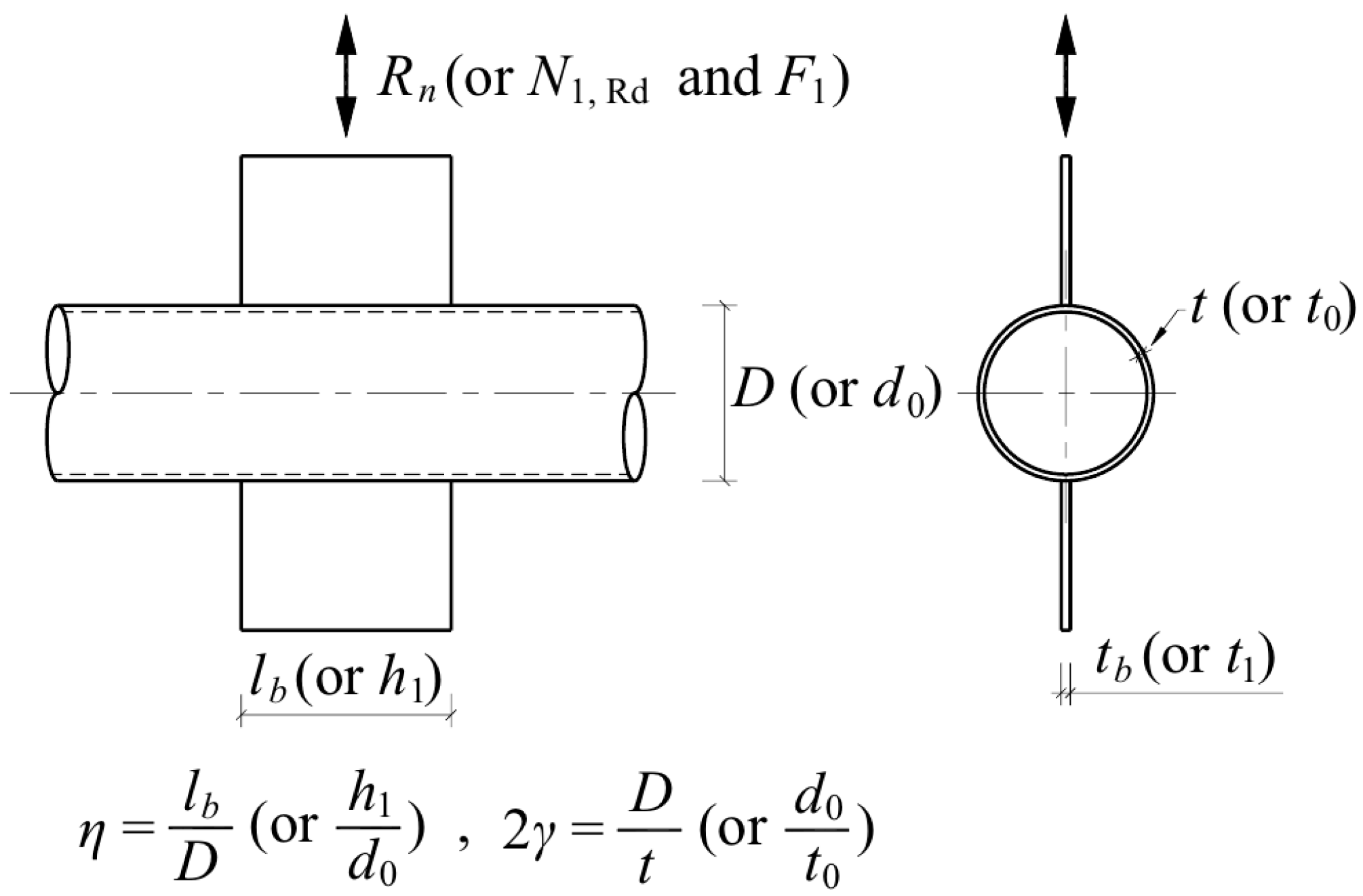
2. Design Equations and Limitations
3. Finite Element Analysis
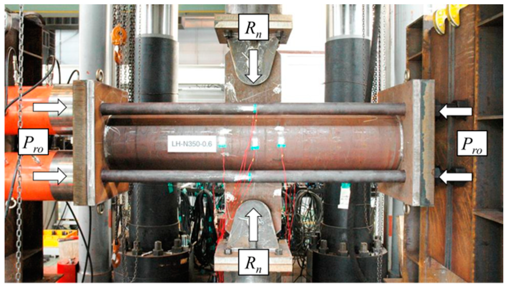
3.1. Finite Element Model
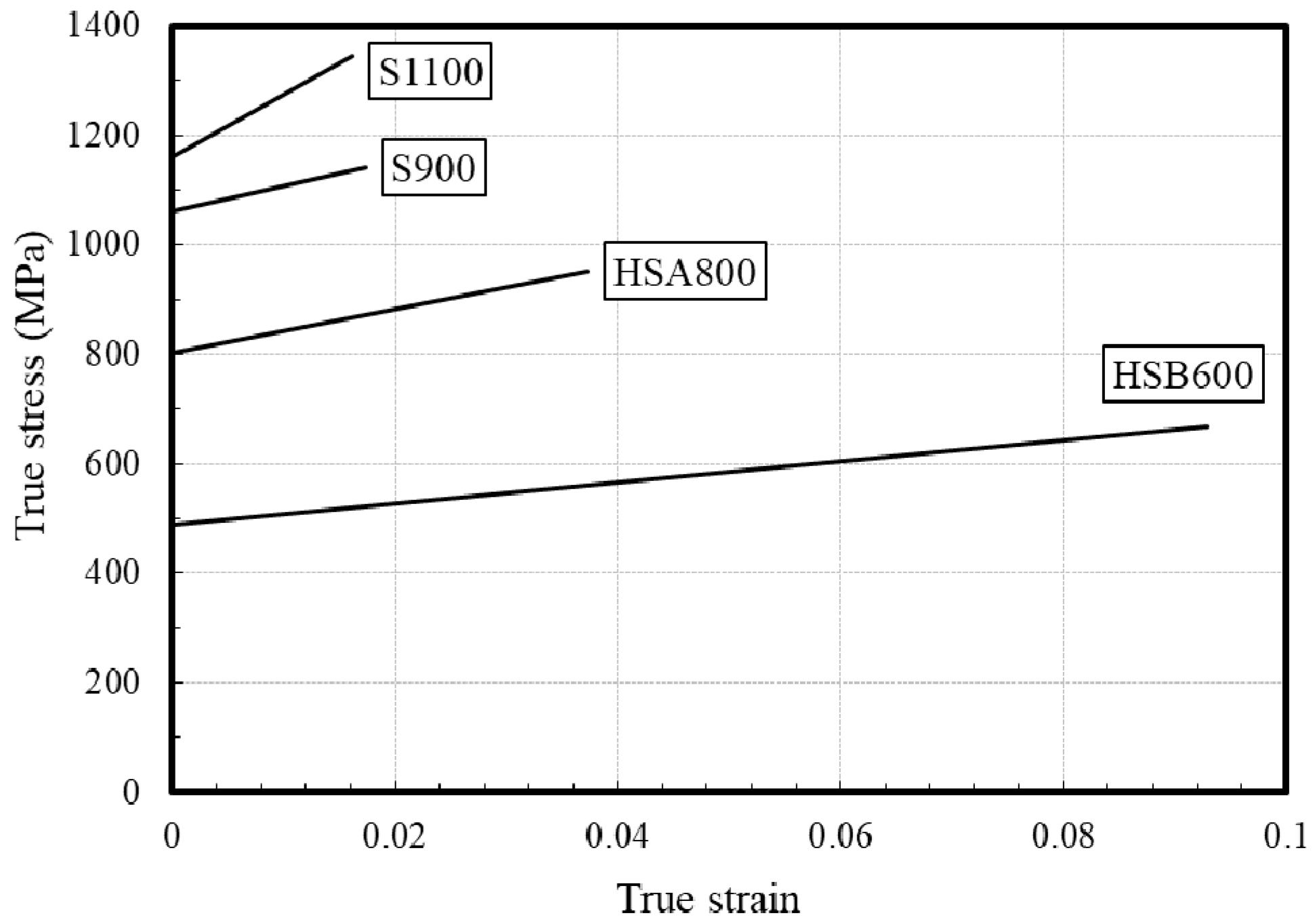
3.2. Material Properties
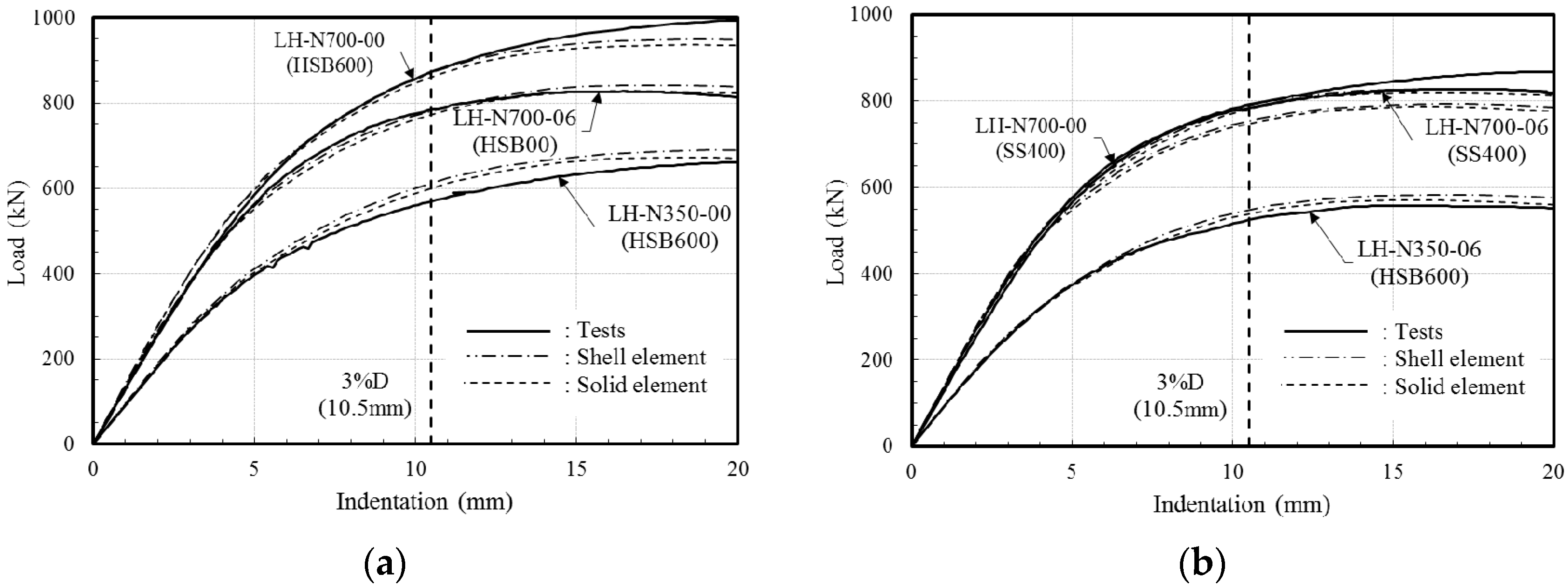
3.3. Mesh Size
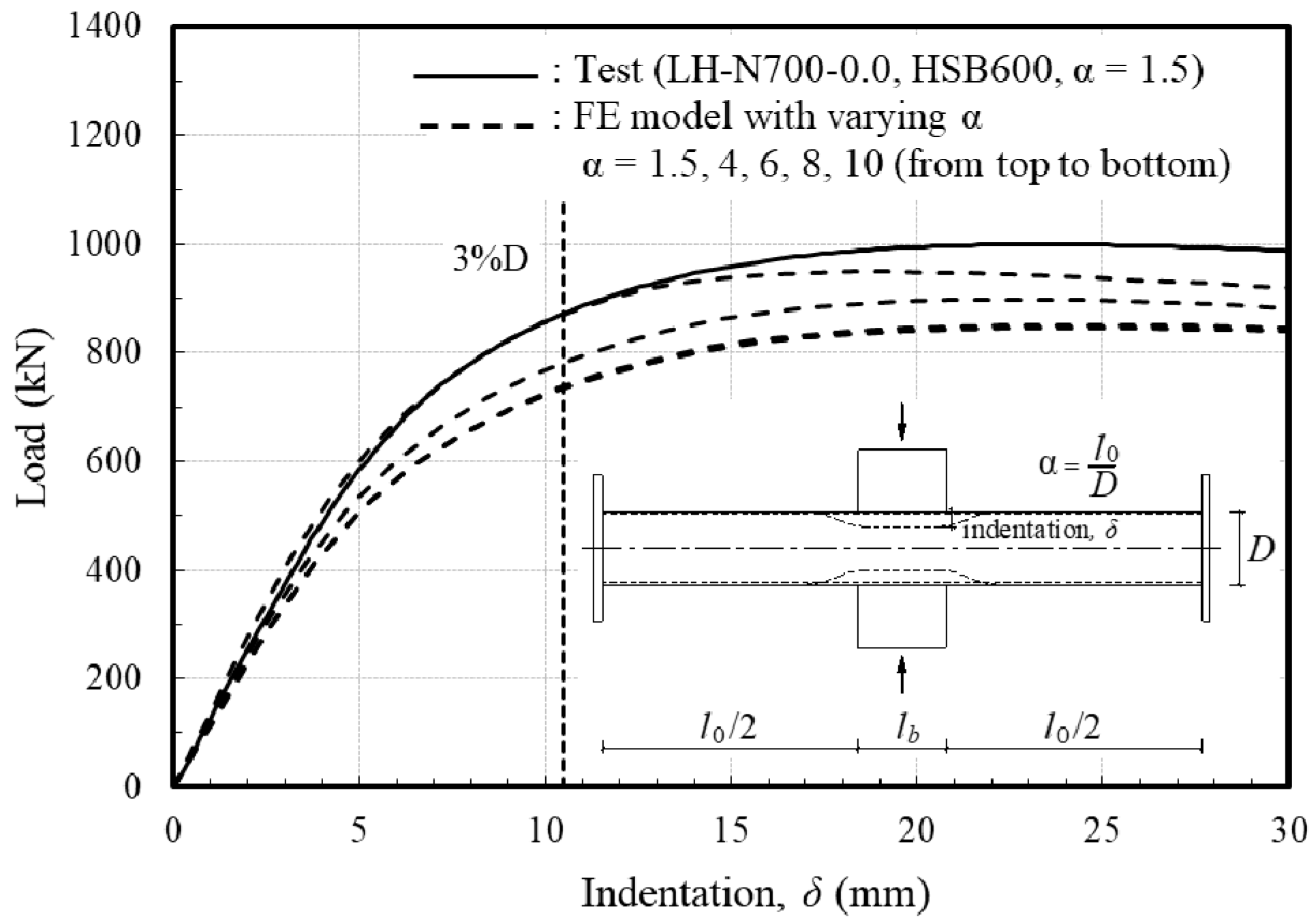
3.4. Chord Length Effect
4. Parametric Analysis
5. Comparison of Design Equations
6. Conclusions
- (1)
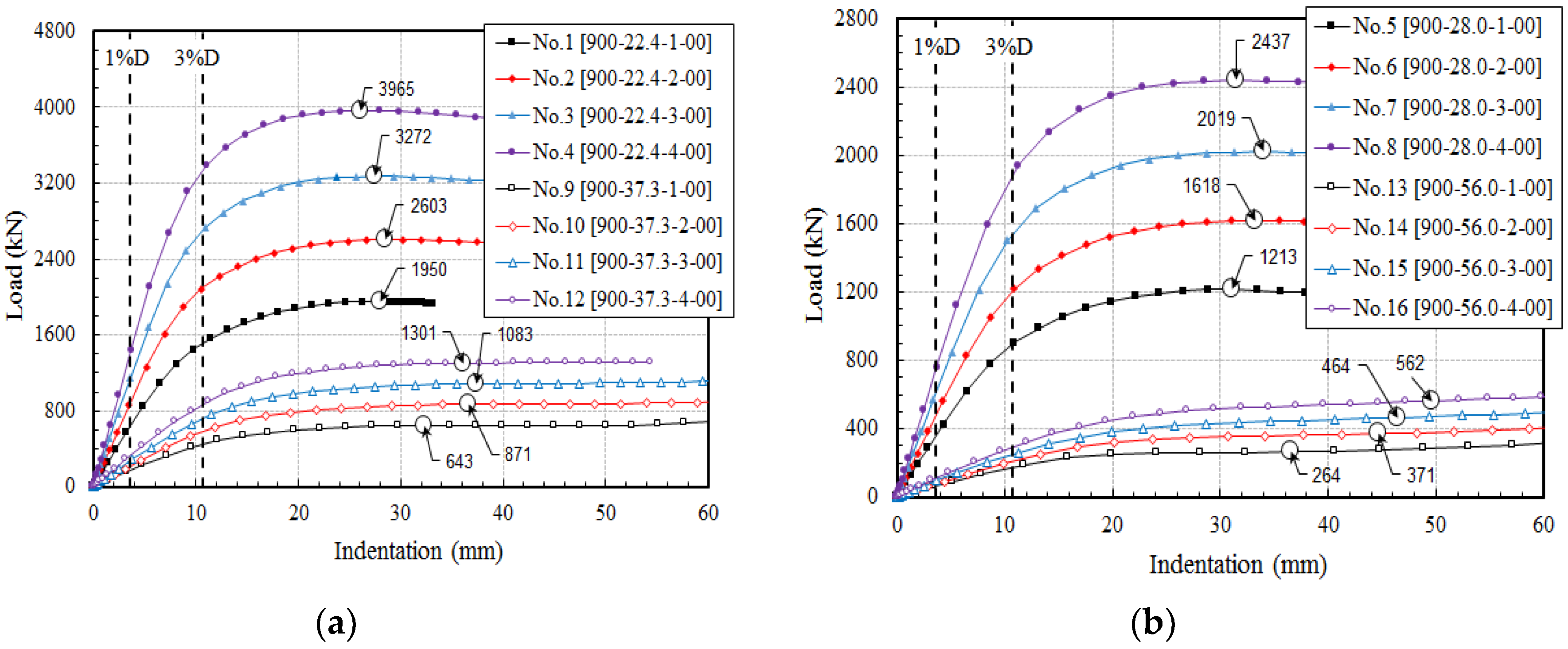
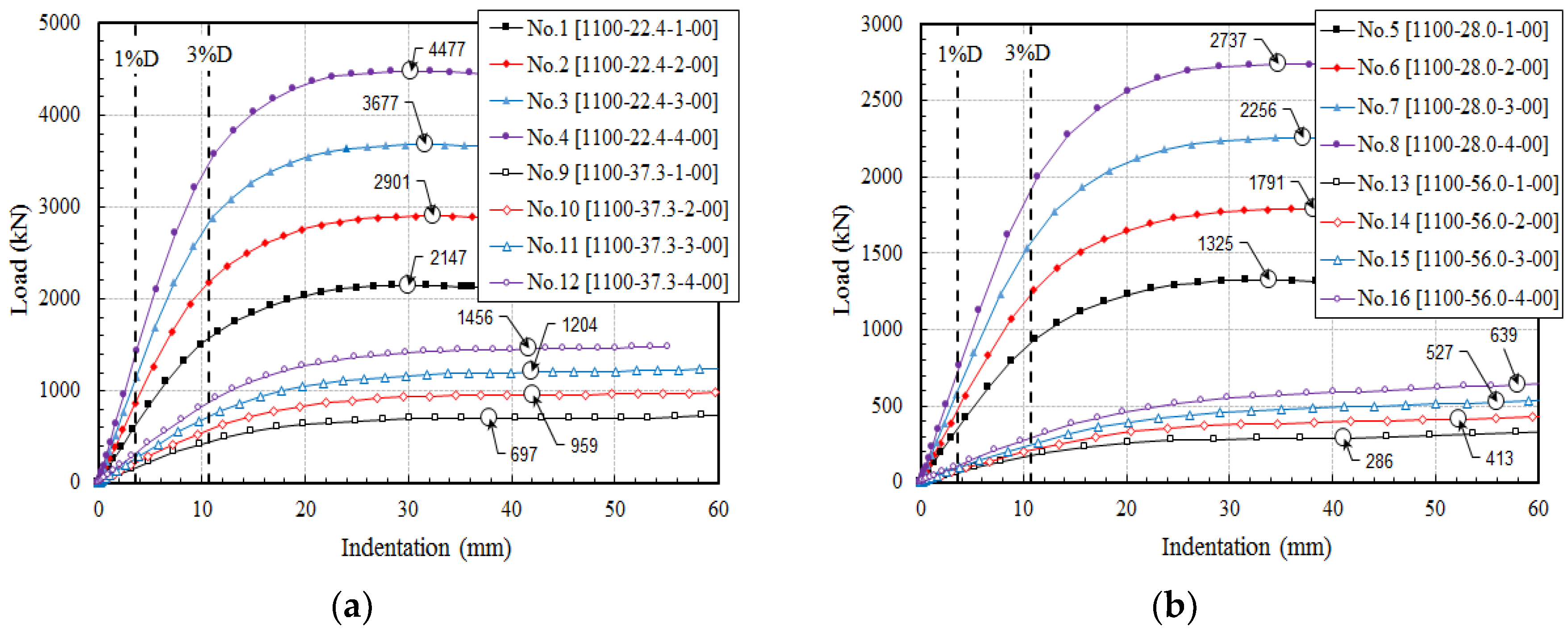
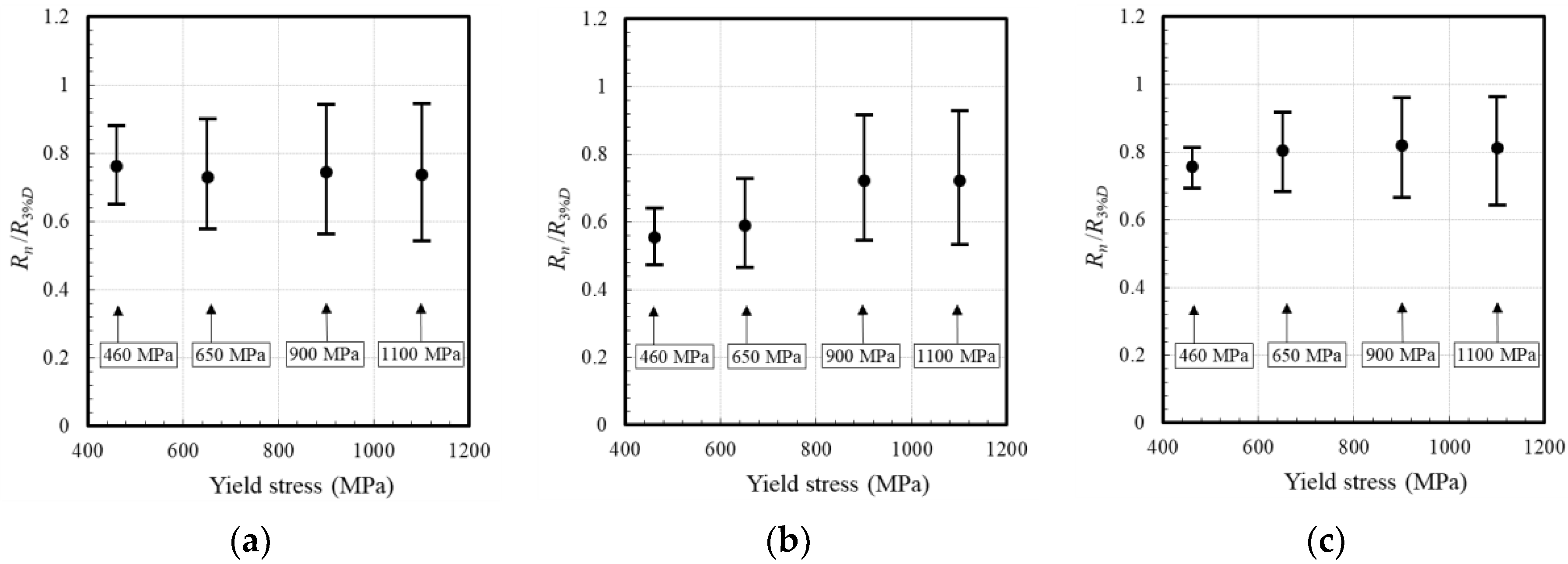
- The joint strength (R3%D) at the ultimate deformation limit is slightly lower than the maximum strength (Rmax) at the yield strength of 460 MPa. The difference between R3%D and Rmax gradually increases, because the R3%D is moved in the elastic region of the load–indentation relationship. However, taking into account the deformation at the Rmax, which has a relatively large connection deformation, the R3%D could be represented as the joint capacity.
- (2)
- The R3%D at yield strengths of 900 and 1100 MPa is almost the same because it belongs to the elastic range. The deformation limit criterion controls the ultimate behavior of the CHS XP-joints, and the elasticity modulus of the material controls the deformation behavior of the joint. This aspect shows that the joint strength determined by the deformation limit converges to a specific level when using higher-strength steels.
- (3)
- The design equations limit the nominal yield strength with different levels in each code. The strength reduction factor can be applied to secure the applicability to high-strength steels while maintaining the design formula. The reduction factors (β), therefore, are suggested for high-strength steel.
- (4)
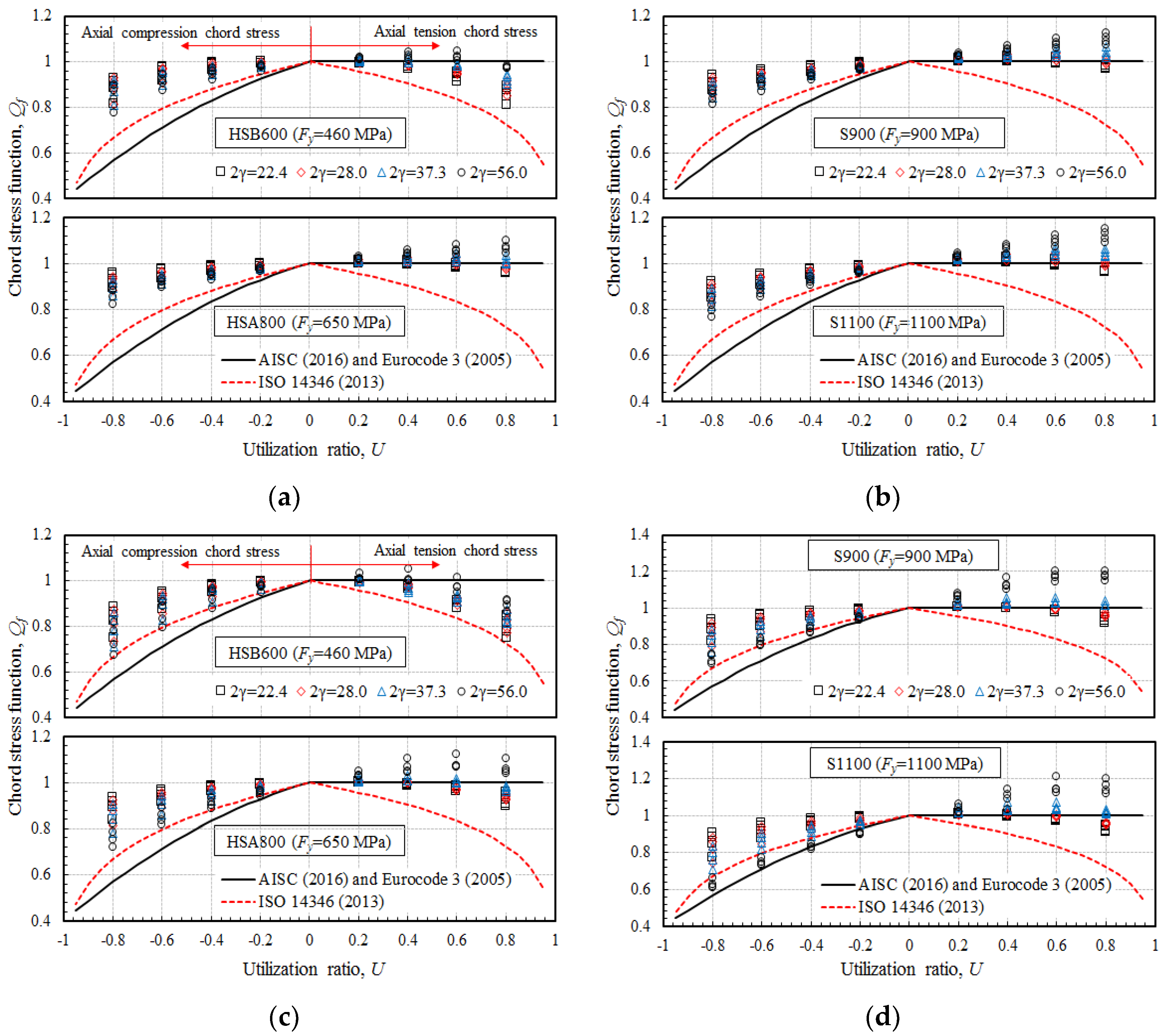
- The chord stress function (Qf) tends to decrease in axial compression chord stress, and it shows a similar tendency to ISO 14346. When the axial tension chord stress is acting on, ISO 14346 is similar at the yield strength of 460 MPa, but AISC and Eurocode 3, which do not consider the strength reduction effect, are similar with increasing yield strength. Therefore, when using the high-strength steel under axial tension chord stress, the strength reduction effect can be neglected.
Author Contributions
Funding
Conflicts of Interest
Glossary
| Ag | Gross cross-section area of chord: |
| D | Diameter of chord (=d0); |
| E | Elastic modulus; |
| Fc | Available stress of chord; |
| Fpl,0 | Chord axial capacity; |
| Fu | Nominal ultimate strength of chord (=σu); |
| Fy | Nominal yield strength of chord (=fy0 and σy0); |
| lb | Width of longitudinal plate (=h1); |
| l0 | Length of chord excluding plate width; |
| Mpl,0 | Chord plastic moment capacity; |
| Mro | Required flexural strength in chord (=M0); |
| Pro | Required axial strength in chord (=F0); |
| Qf | Chord stress interaction parameter (=kp); |
| Qu | Partial design strength function; |
| RFE | Joint strength in finite element analysis; |
| Rmax | Joint strength determined by strength limit state; |
| Rn | Nominal strength of joint (=N1,Rd and F1); |
| Rtest | Joint strength in test; |
| R1%D | Joint strength in serviceability deformation limit; |
| R3%D | Joint strength in ultimate deformation limit; |
| S | Elastic section modulus about the bending axis; |
| s | Weld size; |
| t | Thickness of chord (=t0); |
| tb | Thickness of longitudinal plate (=t1); |
| U | Utilization ratio (=np and n); |
| α | Chord length-to-diameter ratio (=l0/D); |
| β | Reduction factor for high-strength steel; |
| 2γ | Chord diameter-to-thickness ratio (=D/t or d0/t0); |
| εplln | Log strain; |
| εnom | Nominal strain; |
| η | Plate width-to-chord diameter ratio (=lb/D or h1/d0); |
| σnom | Nominal stress; |
| σp,Ed | Maximum compressive stress in the chord; |
| σtrue | True stress; |
| 0.3%D | Chord indentation of joint strength by deformation limit state. |
References
- Wardenier, J. Hollow Section in Structural Applications; Comité International pour le Developpement et l’Etude de la Construction Tubulaire (CIDECT): Geneva, Switzerland, 2001; pp. 1–5. [Google Scholar]
- American Institute of Steel Construction (AISC). Specification for Structural Steel Buildings (AISC 360-16); American Institute of Steel Construction (AISC): Chicago, IL, USA, 2016. [Google Scholar]
- European Committee for Standardization (Eurocode 3). Design of Steel Structures-Part 1–8: Design of Joints; European Committee for Standardization: Brussels, Belgium, 2005. [Google Scholar]
- International Organization for Standardization (ISO 14346). Static Design Procedure for Welded Hollow-Section Joints—Recommendations; International Organization for Standardization: Geneva, Switzerland, 2013. [Google Scholar]
- Togo, T. Experimental Study on Mechanical Behavior of Tubular Joints. Ph.D. Thesis, Osaka University, Osaka, Japan, 1967. [Google Scholar]
- Wardenier, J. Hollow Section Joint; Delft University Press: Delft, The Netherlands, 1982. [Google Scholar]
- Akiyama, N.; Yajima, M.; Akiyama, H.; Ohtake, A. Experimental study on strength of joints in steel tubular structures. J. Soc. J. Steel Constr. 1974, 10, 37–68. [Google Scholar]
- Kurobane, Y.; Makino, Y.; Mitsui, Y. Ultimate strength design formulae for simple tubular joints. IABSE Congr. Rep. Tokyo 1976, 10, 229–234. [Google Scholar] [CrossRef]
- Kurobane, Y. New Developments and Practices in Tubular Joint Design; Doc. XV-488-81; International Institute of Welding: Oporto, Portugal, 1981. [Google Scholar]
- Makino, Y.; Kurobane, Y.; Paul, J.C.; Orita, Y.; Hiraishi, K. Ultimate capacity of gusset plate-to-tube joints under axial and in plane bending loads. In Proceedings of the 4th International Symposium on Tubular Structures, Delft, The Netherlands, 26–28 June 1991. [Google Scholar]
- Architectural Institute of Japan (AIJ). Recommendations for the Design and Fabrication of Tubular Truss Structures in Steel; Architectural Institute of Japan: Tokyo, Japan, 2002. [Google Scholar]
- De Winkel, G.D. The Static Strength of I-beam to Circular Hollow Section Column Connections. Ph.D. Thesis, Delft University of Technology, Delft, The Netherlands, 1998. [Google Scholar]
- Ariyoshi, M.; Wilmshurst, S.R.; Makino, Y. Introduction to the database of gusset-plate to CHS tube joints. In Proceedings of the 8th International Symposium on Tubular Structures, Singapore, 26–28 August 1998. [Google Scholar]
- Wardenier, J.; Kurobane, Y.; Packer, J.A.; van der Vegte, G.J.; Zhao, X.-L. Construction with Hollow Steel Sections. No. 1: Design Guide for Circular Hollow Section (CHS) Joints under Predominantly Static Loading, 2nd ed.; Comité International pour le Developpement et l’Etude de la Construction Tubulaire (CIDECT): Geneva, Switzerland, 2008. [Google Scholar]
- American Petroleum Institute (API). Recommended Practice for Planing, Designing and Constructing Fixed Offshore Platforms-Working Stress Design; American Petroleum Institute: Dallas, TX, USA, 2007. [Google Scholar]
- Pecknold, D.A.; Ha, C.C.; Mohr, W.C. Ultimate strength of DT tubular joints with chord preloads. In Proceedings of the 19th International Conference on Offshore Mechanics and Arctic Engineering, New Orleans, LA, USA, 14–17 February 2000. [Google Scholar]
- Pecknold, D.A.; Marshall, P.W.; Bucknell, J. New API RP2A tubular joint strength design provisions. J. Energy Resour. Technol. 2007, 129, 177–189. [Google Scholar] [CrossRef]
- Ma, J.-L.; Chan, T.-M.; Young, B. Experimental investigation on stub-column behavior of cold-formed high-strength steel tubular sections. J. Struct. Eng. 2016, 142, 04015174. [Google Scholar] [CrossRef]
- Ma, J.-L.; Chan, T.-M.; Young, B. Tests on high-strength steel hollow sections: A review. Struct. Build. 2017, 170, 621–630. [Google Scholar] [CrossRef]
- Puthli, R.; Ummenhofer, T.; Bucak, Ӧ.; Herion, S.; Fleischer, O.; Josat, O. Adaptation and Extension of the Valid Design Formulae for Joints Made of High-Strength Steels up to S690 for Cold-Formed and Hot-Rolled Sections; CIDECT Report 5BT-7/10 (Draft Final Report); CIDECT: Altendorf, Switzerland, 2011. [Google Scholar]
- Lee, C.-H.; Kim, S.-H.; Chung, D.-H.; Kim, D.-K.; Kim, J.-W. Experimental and numerical study of cold-formed high-strength steel CHS X-joints. J. Struct. Eng. 2017, 143, 04017077. [Google Scholar] [CrossRef]
- Lee, C.-H.; Kim, S.-H. Structural performance of CHS X-joints fabricated from high-strength steel. Steel Constr. 2018, 11, 278–285. [Google Scholar] [CrossRef]
- Pandey, B.; Young, B. High strength steel tubular X-joints–an experimental insight under axial compression. In Proceedings of the 16th International Symposium on Tubular Structures, Melbourne, Australia, 4–6 December 2017. [Google Scholar]
- Lan, X.; Chan, T.-M.; Young, B. Static strength of high strength steel CHS X-joints under axial compression. J. Constr. Steel Res. 2017, 138, 369–379. [Google Scholar] [CrossRef]
- Lee, S.-H.; Shin, K.-J.; Lee, H.-D.; Kim, W.-B.; Yang, J.-G. Behavior of plate-to-circular hollow section joints of 600 MPa high-strength steel. Int. J. Steel Struct. 2012, 12, 473–482. [Google Scholar] [CrossRef]
- Lee, S.H.; Shin, K.J.; Lee, H.D.; Kim, W.B. Test and analysis of the longitudinal gusset plate connection to circular hollow section (CHS) of high strength. J. Korean Soc. Steel Constr. 2012, 24, 35–46. [Google Scholar] [CrossRef]
- Kim, W.-B.; Shin, K.-J.; Lee, H.-D.; Lee, S.-H. Strength equations of longitudinal plate-to-circular hollow section (CHS) joints. Int. J. Steel Struct. 2015, 15, 499–505. [Google Scholar] [CrossRef]
- Becque, J.; Wilkinson, T. The capacity of grade C450 cold-formed rectangular hollow section T and X connections: An experimental investigation. J. Constr. Steel Res. 2017, 133, 345–359. [Google Scholar] [CrossRef]
- European Committee for Standardization (Eurocode 3). Design of Steel Structures-Part 1–12: Additional Rules for the Extension of EN 1993 Up to Steel Grades S700; European Committee for Standardization: Brussels, Belgium, 2007. [Google Scholar]
- ABAQUS. Abaqus Analysis User’s Guide (6.13); Dassault Systèmes Simulia Corp.: Johnston, RI, USA, 2013. [Google Scholar]
- Fleischer, O.; Herion, S.; Puthli, R. Numerical investigations on the static behaviour of CHS X joints made of high strength steels. In Proceedings of the 12th International Symposium on Tubular Structures, Shanghai, China, 8–10 October 2008. [Google Scholar]
- Lee, M.M.K.; Wilmshurst, S.R. Numerical modelling of CHS joints with multiplanar double-k configuration. J. Constr. Steel Res. 1994, 32, 281–301. [Google Scholar] [CrossRef]
- Lu, L.H.; de Winkel, G.D.; Yu, Y.; Wardenier, J. Deformation limit for the ultimate strength of hollow section joints. In Proceedings of the 6th International Symposium on Tubular Structures, Melbourne, Australia, 14–16 December 1994. [Google Scholar]
- van der Vegte, G.J.; Makino, Y. Ultimate strength formulation for axially loaded CHS uniplanar T-joints. Int. J. Offshore Polar Eng. 2006, 16, 305–312. [Google Scholar]
- van der Vegte, G.J.; Makino, Y. The effect of chord length and boundary conditions on the static strength of CHS T-and X-joints. In Proceedings of the 5th International Conference on Advances in Steel Structures, Singapore, 5–7 December 2007. [Google Scholar]
- Voth, A.P.; Packer, J.A. Parametric finite element study of branch plate-to-circular hollow section X-connections. In Proceedings of the 12th International Symposium on Tubular Structures, Shanghai, China, 8–10 October 2009. [Google Scholar]
- American Institute of Steel Construction (AISC). Steel Construction Manual, 15th ed.; American Institute of Steel Construction: Chicago, IL, USA, 2017. [Google Scholar]
- American Welding Society (AWS). Specification for Low-Alloy Steel Electrodes for Flux Cored Arc Welding (AWS A5.29/A5.29M:2005), 4th ed.; American Welding Society: Miami, FL, USA, 2005. [Google Scholar]
- Ariyoshi, M.; Makino, Y. Load-deformation relationships for gusset-plate to CHS tube joints under compression loads. Int. J. Offshore Polar Eng. 2000, 10, 292–300. [Google Scholar]
- Choo, Y.S.; Qian, X.D.; Liew, J.Y.R.; Wardenier, J. Static strength of thick-walled CHS X-joints. Part 1. New approach in strength definition. J. Constr. Steel Res. 2003, 59, 1201–1228. [Google Scholar] [CrossRef]


| Factors | AISC (2016) [2] | Eurocode 3 (2005) [3] | ISO 14346 (2013) [4] |
|---|---|---|---|
| Rn (N1,Rd and F1) | 5.5Fyt2(1 + 0.25η)Qf | 5fy0t02(1 + 0.25η)kp | 5σy0t02(1 + 0.4η)Qf |
| Qf (kp) | Chord in tension: 1.0 Chord in compression: 1.0 − 0.3U(1 + U) | Chord in tension: 1.0 Chord in compression: 1.0 − 0.3np(1 + np) ≤ 1.0 | Chord in tension: (1 − |n|)0.20 Chord in compression: (1 − |n|)0.25 |
| Fy (fy0 and σy0) | Fy ≤ 360 MPa | fy0 ≤ 355 MPa: fy0 355 < fy0 ≤ 460 MPa: 0.9fy0 460 < fy0 ≤ 700 MPa: 0.8fy0 | σy0 ≤ 355 MPa: σy0 355 < σy0 ≤ 460 MPa: 0.9σy0 |
| Yield ratio (Fy/Fu) | 0.80 | 0.91 0.95 for fy0 of 460 to 700 MPa | 0.80 If σy0 exceeds 0.8σu, then σy0 = 0.80σu |
| η | − | η ≤ 4 | 1 ≤ η ≤ 4 |
| 2γ | 2γ ≤ 50 | 10 ≤ 2γ ≤ 50 | 2γ ≤ 40 |
| Specimen | Steel Grade | D (mm) | t (mm) | lb (mm) | tb (mm) | Pro (kN) |
|---|---|---|---|---|---|---|
| LH-N700-0.0 1 | SS400 | 350 | 12 | 700 | 12 | 0 |
| LH-N700-0.6 | 1797 | |||||
| LH-N350-0.0 | HSB600 | 350 | 0 | |||
| LH-N350-0.6 | 3364 | |||||
| LH-N700-0.0 | HSB600 | 700 | 0 | |||
| LH-N700-0.6 | 3364 |
| Test | Fy (MPa) | Fu (MPa) | Yield Ratio | Elongation (%) | |
|---|---|---|---|---|---|
| Tensile | SS400 | 356 | 497 | 0.72 | 38.2 |
| HSB600 | 478 | 630 | 0.76 | 34.8 | |
| Stub-column | SS400 | 440 | 487 | 0.90 | - |
| HSB600 | 485 | 606 | 0.80 | - | |
| Element Type | Outside Part of Joint (O.J.) | Joint and Weld Part (J.W.) |
|---|---|---|
| Shell (S4R) and Solid (C3D8R) element | 30 mm | 15 mm |
| 20 mm | 10 mm | |
| 10 mm | 5 mm |
| Specimen | Rtest (kN) | Shell Element | Solid Element | |||||
|---|---|---|---|---|---|---|---|---|
| O.J./J.W. | RFE (kN) | RFE/Rtest | O.J./J.W. | RFE (kN) | RFE/Rtest | |||
| LH-N700-0.0 | SS400 | 791.3 | 20/10 | 788.7 | 1.00 | 20/10 | 780.6 | 0.99 |
| LH-N700-0.6 | 784.0 | 30/15 | 767.0 | 0.98 | 30/15 | 781.2 | 1.00 | |
| LH-N350-0.0 | HSB600 | 569.6 | 10/5 | 611.5 | 1.07 | 10/5 | 600.3 | 1.05 |
| LH-N350-0.6 | 524.5 | 10/5 | 547.7 | 1.04 | 10/5 | 537.8 | 1.03 | |
| LH-N700-0.0 | 872.5 | 20/10 | 870.6 | 1.00 | 20/10 | 861.0 | 0.99 | |
| LH-N700-0.6 | 784.3 | 20/10 | 781.3 | 1.00 | 20/10 | 772.5 | 0.98 | |
| Mean | 1.01 | 1.01 | ||||||
| CoV | 0.033 | 0.026 | ||||||
| Steel | Fy (MPa) | E (MPa) | σ0.2 (MPa) | σu (MPa) | εu (%) |
|---|---|---|---|---|---|
| HSB600 | 460 | 205,000 | 486 | 606 | 10 |
| HSA800 | 650 | 205,000 1 | 798 | 914 | 4.2 1 |
| S900 | 900 | 210,000 | 1054 | 1116 | 2.26 |
| S1100 | 1100 | 207,000 | 1152 | 1317 | 2.20 |
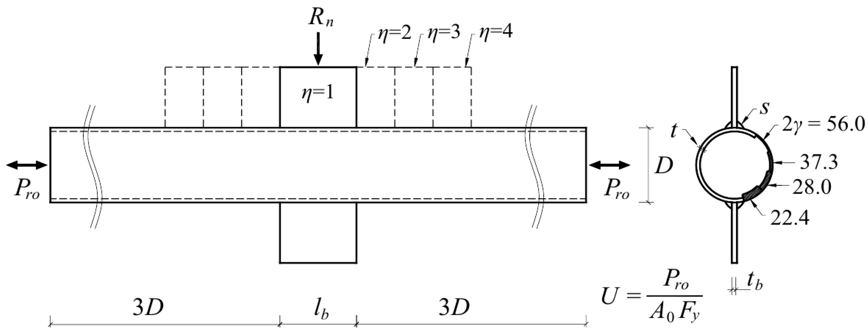
| No. | Specimen (Fy-2γ-η-U) 1 | 2γ (D/t) | η | D (mm) | t, (s) (mm) | lb (mm) |
|---|---|---|---|---|---|---|
| 1 | Fy-22.4-1-U | 22.4 | 1 | 355.6 | 15.875 (10) | 355.6 |
| 2 | Fy-22.4-2-U | 2 | 711.2 | |||
| 3 | Fy-22.4-3-U | 3 | 1066.8 | |||
| 4 | Fy-22.4-4-U | 4 | 1422.4 | |||
| 5 | Fy-28.0-1-U | 28.0 | 1 | 355.6 | 12.7 (8) | 355.6 |
| 6 | Fy-28.0-2-U | 2 | 711.2 | |||
| 7 | Fy-28.0-3-U | 3 | 1066.8 | |||
| 8 | Fy-28.0-4-U | 4 | 1422.4 | |||
| 9 | Fy-37.3-1-U | 37.3 | 1 | 355.6 | 9.525 (6) | 355.6 |
| 10 | Fy-37.3-2-U | 2 | 711.2 | |||
| 11 | Fy-37.3-3-U | 3 | 1066.8 | |||
| 12 | Fy-37.3-4-U | 4 | 1422.4 | |||
| 13 | Fy-56.0-1-U | 56.0 | 1 | 355.6 | 6.35 (6) | 355.6 |
| 14 | Fy-56.0-2-U | 2 | 711.2 | |||
| 15 | Fy-56.0-3-U | 3 | 1066.8 | |||
| 16 | Fy-56.0-4-U | 4 | 1422.4 |
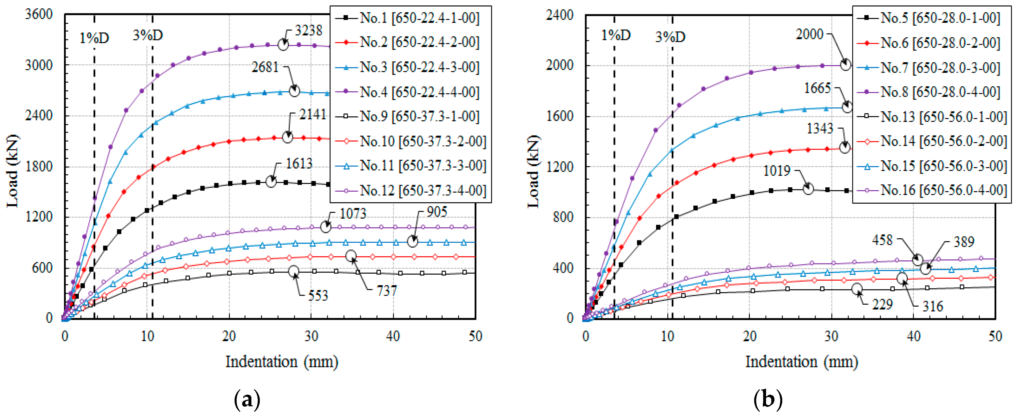
| No. | Specimen (Fy-2γ-η-U) | R1%D (kN) | R3%D (kN) | R3%D/R1%D | Rmax (kN) | Rmax/R3%D | Det. 2 | |
|---|---|---|---|---|---|---|---|---|
| 1 | 460-22.4-1-00 | 577.2 | 987.3 | 1.71 | 1076.0 | (5.7) 1 | 1.09 | F.P. |
| 2 | 460-22.4-2-00 | 811.3 | 1290.7 | 1.59 | 1402.8 | (6.2) | 1.09 | F.P. |
| 3 | 460-22.4-3-00 | 1047.3 | 1616.1 | 1.54 | 1734.9 | (6.8) | 1.07 | F.P. |
| 4 | 460-22.4-4-00 | 1288.2 | 1956.3 | 1.52 | 2076.0 | (6.3) | 1.06 | F.P. |
| 5 | 460-28.0-1-00 | 331.2 | 610.7 | 1.84 | 695.8 | (5.7) | 1.14 | F.P. |
| 6 | 460-28.0-2-00 | 444.0 | 790.0 | 1.78 | 896.8 | (7.1) | 1.14 | F.P. |
| 7 | 460-28.0-3-00 | 570.9 | 983.0 | 1.72 | 1095.6 | (6.7) | 1.11 | F.P. |
| 8 | 460-28.0-4-00 | 694.5 | 1182.2 | 1.70 | 1301.2 | (6.8) | 1.10 | F.P. |
| 9 | 460-37.3-1-00 | 162.8 | 325.5 | 2.00 | 390.9 | (6.4) | 1.20 | F.P. |
| 10 | 460-37.3-2-00 | 207.5 | 415.3 | 2.00 | 507.8 | (7.7) | 1.22 | F.P. |
| 11 | 460-37.3-3-00 | 258.3 | 511.1 | 1.98 | 610.7 | (8.5) | 1.19 | F.P. |
| 12 | 460-37.3-4-00 | 309.6 | 613.4 | 1.98 | 717.7 | (8.5) | 1.17 | F.P. |
| 13 | 460-56.0-1-00 | 63.4 | 138.0 | 2.18 | 168.2 | (5.8) | 1.22 | F.P. |
| 14 | 460-56.0-2-00 | 74.8 | 172.2 | 2.30 | 225.8 | (7.8) | 1.31 | P.W. |
| 15 | 460-56.0-3-00 | 88.6 | 204.8 | 2.31 | 265.1 | (7.5) | 1.29 | P.W. |
| 16 | 460-56.0-4-00 | 103.6 | 241.8 | 2.33 | 308.8 | (7.8) | 1.28 | P.W. |
| No. | Specimen (Fy-2γ-η-U) | R1%D (kN) | R3%D (kN) | R3%D/R1%D | Rmax (kN) | Rmax/R3%D | Det. | |
|---|---|---|---|---|---|---|---|---|
| 1 | 650-22.4-1-00 | 615.6 | 1312.4 | 2.13 | 1613.4 | (7.1) | 1.23 | F.P. |
| 2 | 650-22.4-2-00 | 859.2 | 1786.7 | 2.08 | 2141.0 | (7.7) | 1.20 | F.P. |
| 3 | 650-22.4-3-00 | 1110.9 | 2289.7 | 2.06 | 2681.4 | (7.9) | 1.17 | F.P. |
| 4 | 650-22.4-4-00 | 1366.1 | 2808.3 | 2.06 | 3238.1 | (7.5) | 1.15 | F.P. |
| 5 | 650-28.0-1-00 | 345.1 | 784.5 | 2.27 | 1018.8 | (7.7) | 1.30 | F.P. |
| 6 | 650-28.0-2-00 | 461.5 | 1051.8 | 2.28 | 1343.1 | (8.9) | 1.28 | F.P. |
| 7 | 650-28.0-3-00 | 587.7 | 1339.8 | 2.28 | 1665.2 | (9.0) | 1.24 | F.P. |
| 8 | 650-28.0-4-00 | 715.5 | 1626.1 | 2.27 | 1999.8 | (9.0) | 1.23 | F.P. |
| 9 | 650-37.3-1-00 | 165.5 | 404.5 | 2.44 | 552.7 | (7.9) | 1.37 | F.P. |
| 10 | 650-37.3-2-00 | 210.8 | 526.5 | 2.50 | 736.8 | (9.8) | 1.40 | F.P. |
| 11 | 650-37.3-3-00 | 261.4 | 657.1 | 2.51 | 904.8 | (11.9) | 1.38 | F.P. |
| 12 | 650-37.3-4-00 | 313.5 | 795.4 | 2.54 | 1073.4 | (9.0) | 1.35 | P.W. |
| 13 | 650-56.0-1-00 | 63.5 | 163.5 | 2.58 | 229.3 | (9.4) | 1.40 | P.W. |
| 14 | 650-56.0-2-00 | 75.0 | 199.8 | 2.66 | 315.9 | (10.9) | 1.58 | P.W. |
| 15 | 650-56.0-3-00 | 88.8 | 237.2 | 2.67 | 388.7 | (11.7) | 1.64 | P.W. |
| 16 | 650-56.0-4-00 | 104.0 | 279.2 | 2.69 | 458.0 | (11.4) | 1.64 | P.W. |
| No. | Specimen (Fy-2γ-η-U) | R1%D (kN) | R3%D (kN) | R3%D/R1%D | Rmax (kN) | Rmax/R3%D | Det. | |
|---|---|---|---|---|---|---|---|---|
| 1 | 900-22.4-1-00 | 634.5 | 1508.9 | 2.38 | 1950.4 | (7.9) | 1.29 | F.P. |
| 2 | 900-22.4-2-00 | 882.1 | 2092.1 | 2.37 | 2602.6 | (8.0) | 1.24 | F.P. |
| 3 | 900-22.4-3-00 | 1141.5 | 2704.1 | 2.37 | 3271.5 | (7.7) | 1.21 | F.P. |
| 4 | 900-22.4-4-00 | 1403.2 | 3327.5 | 2.37 | 3964.5 | (7.3) | 1.19 | F.P. |
| 5 | 900-28.0-1-00 | 354.5 | 890.1 | 2.51 | 1213.4 | (8.8) | 1.36 | F.P. |
| 6 | 900-28.0-2-00 | 474.1 | 1204.7 | 2.54 | 1618.4 | (9.3) | 1.34 | F.P. |
| 7 | 900-28.0-3-00 | 602.5 | 1532.2 | 2.54 | 2018.8 | (9.6) | 1.32 | F.P. |
| 8 | 900-28.0-4-00 | 733.8 | 1874.1 | 2.55 | 2436.6 | (8.8) | 1.30 | F.P. |
| 9 | 900-37.3-1-00 | 169.7 | 446.1 | 2.63 | 643.4 | (9.1) | 1.44 | F.P. |
| 10 | 900-37.3-2-00 | 216.1 | 575.3 | 2.66 | 871.4 | (10.3) | 1.51 | P.W. |
| 11 | 900-37.3-3-00 | 267.8 | 717.4 | 2.68 | 1083.3 | (10.5) | 1.51 | P.W. |
| 12 | 900-37.3-4-00 | 321.4 | 867.0 | 2.70 | 1301.4 | (10.6) | 1.50 | P.W. |
| 13 | 900-56.0-1-00 | 65.0 | 174.9 | 2.69 | 263.6 | (10.3) | 1.51 | P.W. |
| 14 | 900-56.0-2-00 | 76.8 | 210.3 | 2.74 | 371.1 | (12.6) | 1.76 | P.W. |
| 15 | 900-56.0-3-00 | 91.0 | 249.9 | 2.75 | 464.2 | (13.1) | 1.86 | P.W. |
| 16 | 900-56.0-4-00 | 106.5 | 293.4 | 2.76 | 562.5 | (14.0) | 1.92 | P.W. |
| No. | Specimen (Fy-2γ-η-U) | R1%D (kN) | R3%D (kN) | R3%D/R1%D | Rmax(kN) | Rmax/R3%D | Det. | |
|---|---|---|---|---|---|---|---|---|
| 1 | 1100-22.4-1-00 | 626.0 | 1569.5 | 2.51 | 2146.6 | (8.5) | 1.37 | F.P. |
| 2 | 1100-22.4-2-00 | 870.1 | 2185.7 | 2.51 | 2901.0 | (9.1) | 1.33 | F.P. |
| 3 | 1100-22.4-3-00 | 1125.1 | 2824.8 | 2.51 | 3676.7 | (8.9) | 1.30 | F.P. |
| 4 | 1100-22.4-4-00 | 1383.0 | 3479.9 | 2.52 | 4477.4 | (8.5) | 1.29 | F.P. |
| 5 | 1100-28.0-1-00 | 349.5 | 912.3 | 2.61 | 1324.8 | (9.5) | 1.45 | F.P. |
| 6 | 1100-28.0-2-00 | 467.3 | 1228.2 | 2.63 | 1791.3 | (10.8) | 1.46 | F.P. |
| 7 | 1100-28.0-3-00 | 594.2 | 1566.8 | 2.64 | 2256.0 | (10.4) | 1.44 | F.P. |
| 8 | 1100-28.0-4-00 | 723.2 | 1911.1 | 2.64 | 2736.8 | (9.8) | 1.43 | F.P. |
| 9 | 1100-37.3-1-00 | 167.3 | 449.5 | 2.69 | 697.5 | (10.6) | 1.55 | F.P. |
| 10 | 1100-37.3-2-00 | 213.0 | 578.1 | 2.71 | 958.7 | (11.8) | 1.66 | P.W. |
| 11 | 1100-37.3-3-00 | 264.0 | 720.4 | 2.73 | 1203.5 | (11.8) | 1.67 | P.W. |
| 12 | 1100-37.3-4-00 | 316.8 | 869.7 | 2.75 | 1455.6 | (12.2) | 1.67 | P.W. |
| 13 | 1100-56.0-1-00 | 64.1 | 174.0 | 2.72 | 286.5 | (11.6) | 1.65 | P.W. |
| 14 | 1100-56.0-2-00 | 75.7 | 208.7 | 2.76 | 412.7 | (14.7) | 1.98 | P.W. |
| 15 | 1100-56.0-3-00 | 89.7 | 247.7 | 2.76 | 527.1 | (15.8) | 2.13 | P.W. |
| 16 | 1100-56.0-4-00 | 105.0 | 290.9 | 2.77 | 639.2 | (16.3) | 2.20 | P.W. |
| No. | Normalized Joint Strength, R3%D/Fyt2 | AISC (2016) [2] | Eurocode (2005) [3] 1 | ISO 14346 (2013) [4] 2 | |||||||||||||||
|---|---|---|---|---|---|---|---|---|---|---|---|---|---|---|---|---|---|---|---|
| Yield Stress of CHS | Rn/Fyt2 | Rn/R3%D | N1,Rd/Fyt2 | N1,Rd/R3%D | F1/Fyt2 | F1/R3%D | |||||||||||||
| 460 | 650 | 900 | 1100 | 460 | 650 | 900 | 1100 | 460 | 650 | 900 | 1100 | 460 | 650 | 900 | 1100 | ||||
| 1 | 8.5 | 8.0 | 6.7 | 5.7 | 6.9 | 0.8 | 0.9 | 1.0 | 1.2 | 5.0 | 0.6 | 0.6 | 0.8 | 0.9 | 6.3 | 0.7 | 0.8 | 0.9 | 1.1 |
| 2 | 11.1 | 10.9 | 9.2 | 7.9 | 8.3 | 0.7 | 0.8 | 0.9 | 1.0 | 6.0 | 0.5 | 0.6 | 0.7 | 0.8 | 8.1 | 0.7 | 0.7 | 0.9 | 1.0 |
| 3 | 13.9 | 14.0 | 11.9 | 10.2 | 9.6 | 0.7 | 0.7 | 0.8 | 0.9 | 7.0 | 0.5 | 0.5 | 0.6 | 0.7 | 9.9 | 0.7 | 0.7 | 0.8 | 1.0 |
| 4 | 16.9 | 17.1 | 14.7 | 12.6 | 11.0 | 0.7 | 0.6 | 0.7 | 0.9 | 8.0 | 0.5 | 0.5 | 0.5 | 0.6 | 11.7 | 0.7 | 0.7 | 0.8 | 0.9 |
| 5 | 8.2 | 7.5 | 6.1 | 5.1 | 6.9 | 0.8 | 0.9 | 1.1 | 1.3 | 5.0 | 0.6 | 0.7 | 0.8 | 1.0 | 6.3 | 0.8 | 0.8 | 1.0 | 1.2 |
| 6 | 10.6 | 10.0 | 8.3 | 6.9 | 8.3 | 0.8 | 0.8 | 1.0 | 1.2 | 6.0 | 0.6 | 0.6 | 0.7 | 0.9 | 8.1 | 0.8 | 0.8 | 1.0 | 1.2 |
| 7 | 13.2 | 12.8 | 10.6 | 8.8 | 9.6 | 0.7 | 0.8 | 0.9 | 1.1 | 7.0 | 0.5 | 0.5 | 0.7 | 0.8 | 9.9 | 0.7 | 0.8 | 0.9 | 1.1 |
| 8 | 15.9 | 15.5 | 12.9 | 10.8 | 11.0 | 0.7 | 0.7 | 0.9 | 1.0 | 8.0 | 0.5 | 0.5 | 0.6 | 0.7 | 11.7 | 0.7 | 0.8 | 0.9 | 1.1 |
| 9 | 7.8 | 6.9 | 5.5 | 4.5 | 6.9 | 0.9 | 1.0 | 1.3 | 1.5 | 5.0 | 0.6 | 0.7 | 0.9 | 1.1 | 6.3 | 0.8 | 0.9 | 1.2 | 1.4 |
| 10 | 10.0 | 8.9 | 7.0 | 5.8 | 8.3 | 0.8 | 0.9 | 1.2 | 1.4 | 6.0 | 0.6 | 0.7 | 0.9 | 1.0 | 8.1 | 0.8 | 0.9 | 1.1 | 1.4 |
| 11 | 12.2 | 11.1 | 8.8 | 7.2 | 9.6 | 0.8 | 0.9 | 1.1 | 1.3 | 7.0 | 0.6 | 0.6 | 0.8 | 1.0 | 9.9 | 0.8 | 0.9 | 1.1 | 1.4 |
| 12 | 14.7 | 13.5 | 10.6 | 8.7 | 11.0 | 0.7 | 0.8 | 1.0 | 1.3 | 8.0 | 0.5 | 0.6 | 0.8 | 0.9 | 11.7 | 0.8 | 0.9 | 1.1 | 1.3 |
| 13 | 7.4 | 6.2 | 4.8 | 3.9 | 6.9 | 0.9 | 1.1 | 1.4 | 1.8 | 5.0 | 0.7 | 0.8 | 1.0 | 1.3 | 6.3 | 0.8 | 1.0 | 1.3 | 1.6 |
| 14 | 9.3 | 7.6 | 5.8 | 4.7 | 8.3 | 0.9 | 1.1 | 1.4 | 1.8 | 6.0 | 0.6 | 0.8 | 1.0 | 1.3 | 8.1 | 0.9 | 1.1 | 1.4 | 1.7 |
| 15 | 11.0 | 9.1 | 6.9 | 5.6 | 9.6 | 0.9 | 1.1 | 1.4 | 1.7 | 7.0 | 0.6 | 0.8 | 1.0 | 1.3 | 9.9 | 0.9 | 1.1 | 1.4 | 1.8 |
| 16 | 13.0 | 10.7 | 8.1 | 6.6 | 11.0 | 0.8 | 1.0 | 1.4 | 1.7 | 8.0 | 0.6 | 0.8 | 1.0 | 1.2 | 11.7 | 0.9 | 1.1 | 1.4 | 1.8 |
| Mean | 0.79 | 0.88 | 1.10 | 1.32 | 0.58 | 0.64 | 0.80 | 0.96 | 0.79 | 0.87 | 1.09 | 1.32 | |||||||
| CoV | 0.101 | 0.168 | 0.206 | 0.223 | 0.101 | 0.168 | 0.206 | 0.223 | 0.082 | 0.155 | 0.197 | 0.215 | |||||||
© 2019 by the authors. Licensee MDPI, Basel, Switzerland. This article is an open access article distributed under the terms and conditions of the Creative Commons Attribution (CC BY) license (http://creativecommons.org/licenses/by/4.0/).
Share and Cite
Lee, S.-H.; Shin, K.-J.; Kim, S.-Y.; Lee, H.-D. Numerical Study on the Deformation Behavior of Longitudinal Plate-to-High-Strength Circular Hollow-Section X-Joints under Axial Load. Appl. Sci. 2019, 9, 3999. https://doi.org/10.3390/app9193999
Lee S-H, Shin K-J, Kim S-Y, Lee H-D. Numerical Study on the Deformation Behavior of Longitudinal Plate-to-High-Strength Circular Hollow-Section X-Joints under Axial Load. Applied Sciences. 2019; 9(19):3999. https://doi.org/10.3390/app9193999
Chicago/Turabian StyleLee, Swoo-Heon, Kyung-Jae Shin, So-Yeong Kim, and Hee-Du Lee. 2019. "Numerical Study on the Deformation Behavior of Longitudinal Plate-to-High-Strength Circular Hollow-Section X-Joints under Axial Load" Applied Sciences 9, no. 19: 3999. https://doi.org/10.3390/app9193999
APA StyleLee, S.-H., Shin, K.-J., Kim, S.-Y., & Lee, H.-D. (2019). Numerical Study on the Deformation Behavior of Longitudinal Plate-to-High-Strength Circular Hollow-Section X-Joints under Axial Load. Applied Sciences, 9(19), 3999. https://doi.org/10.3390/app9193999