Featured Application
The outcome of this study may beneficial to the researchers, engineers, designers while dealing with the motion of single bubbles in still water.
Abstract
Under the action of gravity, buoyancy, and surface tension, bubbles generated by wave breaking will rupture and polymerize, causing the occurrence of high-speed jets and strong turbulence in nearby water bodies, which in turn affects sea–air exchange, sediment transport, and pollutant movement. These interactions are closely related to the shape and velocity changes in single bubbles. Therefore, understanding the motion characteristics of single bubbles is essential. In this research, a large number of experiments were carried out to serve this purpose. The experimental data were used to develop three machine learning models for the bubble final velocity, bubble drag coefficient, and bubble shape, respectively. The performance of the feed forward back propagation neural network (FBNN) models for the final velocity and drag coefficient were evaluated. The coefficient of determination (R2) and root mean squared error (RMSE) value of final velocity prediction model was recorded at 0.83 and 0.0518, respectively. Meanwhile, for the drag coefficient prediction model, the values are 0.92 for R2 and 0.1534 for RMSE. The models can provide a more accurate output if compared to that from the empirical formulas. K-nearest neighbours (KNN), logistic regression, and random forest were applied as the algorithm while developing the bubble shape classification model. The best performance is achieved by the logistic regression.
1. Introduction
1.1. Background
Gas–liquid two-phase flow widely exists in nature. It plays an important role in engineering applications, especially while dealing with the problems related to sea–air exchange, cavitation of buildings due to the high-speed dam water, natural gas transportation, etc. Under the effect of gravitational force, buoyancy force, and surface tension, the bubbles may experience a change in shape, breakage, as well as merging. These scenarios will lead to the occurrences of high-speed jets and strong turbulence in the water bodies nearby, which affect the mechanism of sea–air exchange and pollutant movement. These interactions are closely related to the states and nature of single bubbles. Therefore, it is essential to have an understanding of the motion characteristics of single bubbles in order to study its effect on sea–air flux exchange, stress exerted on the building structures, and provide a fundamental theoretical basis for the development of marine engineering.
In most of the natural phenomena, as well as real-life practical applications, bubbles in water bodies play a significant role. Based on the previous analyses, the phenomena such as underwater sound wave propagation, atmospheric–marine gas exchange, ship navigation, laser transmission underwater, nutrient supply for marine life, etc., had shown a close relationship with the motion characteristics of single bubbles in the water [1].
Bubbles can be formed through different processes such as wave rolling, ocean biological activities, ship navigation, etc. The existing scientific evidence had proved that the gases entrained by breaking wave contained 30% of human-generated CO2, which may help to alleviate the global warming issue. In addition, the splash and entrainment due to the breaking wave can enhance the exchange of heat, water vapour, gas, and energy in the sea.
On the other hand, the acoustic characteristic of the bubbles on the ocean surface layer is one of the most eye-catching issues. A large number of bubbles resulting from the breaking wave will cause a great impact on the optical properties of seawater. It will scatter the light and affect the remote sensing information of the sea surface [2]. Hence, studying the motion characteristics of the single bubbles has an important theoretical and scientific significance for the mechanisms of two-phase flow.
1.2. Problem Statement
In the past, to study the kinematic and dynamic mechanisms of single bubbles, the researchers used the theoretical analyses as well as a simplified model. Among all, Lord Rayleigh [3] was the first who assumed the liquid is incompressible, non-viscous, and non-rotating. With the assumption, he proposed a bubble transport equation. Such an equation has become the basis for the study of bubbles. It was widely applied and improved by the other researchers [4,5,6,7,8,9].
In general, the relationship among the motion characteristics of single bubbles and their relationships with the external forces are complicated. It is hard to describe the mechanisms of single bubbles by using only the theoretical analyses. Hence, laboratory work is essential, especially in observing and analysing the process of bubble rise. The widely used experimental approaches to observe the upward movement of single bubbles in still water are photographing method, particle image velocimetry (PIV) measurement, conductance proves, pressure sensing, and others [10,11,12,13,14,15,16,17,18].
However, due to certain limitations of the experimental instruments, the knowledge of single bubbles is still limited. This is because it is difficult to measure the single bubble motion and the flow pattern of the surrounding liquid without any interference.
Therefore, there is a need to have an alternative approach which is able to serve as a basis for the further exploration of single bubble motion and transport mechanisms under the breaking wave condition.
1.3. Motivation
Machine learning has a wide application. Feed forward back propagation neural network is one of the popular machine learning approaches [19]. It has the ability to overcome the constraints of the existing mathematical models and helps in problem-solving based on the complementary nature of both modelling and practices.
In addition, machine learning has played an important role in water-related engineering applications, such as reservoir operation [20,21], water management [22,23], turbine operation [24,25], water distribution network [26,27], sediment settling velocity prediction [28], intelligence hydrological model [29,30], rheological prediction model [31,32] etc. Therefore, it is believed that such a method is also applicable for the study of motion characteristics of the single bubbles.
By formulating machine learning models that are able to predict the final velocity, drag coefficient, and shape of single bubbles with an acceptable level of accuracy, it may beneficial to the researchers, engineers, and hydrologists while dealing with the issues related to bubbles.
1.4. Research Objectives
The major aim of this research is, through a machine learning approach, to propose machine learning models which can provide a basis for the single bubble motion and transport mechanism under breaking wave conditions. The proposed models were developed based on the experimental data obtained from laboratory works. During the training process, Reynold (Re) number, Eotvos (Eo) number, and Weber (We) number, all of which are the critical elements influencing motion characteristics of single bubbles, were kept as the input parameters. This study is innovative in its use of the machine learning approach to predict the final velocity, drag coefficient, and shape of single bubbles in still water.
2. Materials and Methods
Digital image measurement has been widely used in the field of two-phase flow due to its unique characteristics. It has the ability to visualise the motion of single bubbles without showing any disturbance to the flow field. In this study, the high-speed camera was used to capture the whole processes of bubbles production, motion, and deformation in still water.
2.1. Laboratory Experiment
First of all, a special tank was designed using rectangular transparent plexiglass. The top was connected to the atmosphere to create a normal pressure state, as shown in Figure 1. There was also a bubble generating device and a drain setting at the bottom of the tank.
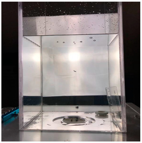
Figure 1.
Special-designed tank.
Tap water with a water level of 250 mm was poured into the tank. The experiments were started only after the water surface calmed and the water temperature reached the same level as room temperature.
A peristaltic pump was used to control gas production. It is a must ensure a suitable flow rate for the generation of the bubbles. This is because, at a low flow rate condition, the formation of the bubbles is very slow, and thereby it is difficult to detach at the orifice and causes the liquid to flow into the orifice easily. Meanwhile, if the flow rate is too large, the frequency of bubbles generation will be very fast, and it is hard to form single bubbles under such conditions. The equivalent diameter of the bubbles ranged from2 to 7.5 mm, while the periodic injection mode was selected. In order to ensure the periodicity, the detachment frequency, which represented the number of bubbles per unit time, was kept constant throughout the experiments.
On the other hand, in order to clearly capture the whole evolution process of single bubbles, a high-speed two-dimensional camera was set on the side of the bubble’s generation section. A three-colour soft light with the standard colour temperature and light brightness was used to smoothen the image capturing process.
The experiments were carried out in a dark room under different flow rate, breakaway frequency, and needle size (to control the size of bubble) conditions. The physical properties of the tested samples are shown in Table 1.

Table 1.
Properties of tested samples.
2.2. Data Extraction
The motion of single bubbles is closely related to several factors, such as frequency of separation, physical properties of the liquid, size of the bubble, and shape of the bubble. The dynamic and kinematic characteristics of single bubbles in the still water were studied by changing the bubble detachment frequency and the orifice diameter in the specially designed tank.
Digital image processing was used to extract the data such as bubble velocity, drag force coefficient, and bubble shape from the images captured during the experiments. The shape categorisation of the bubbles is basically based on the aspect ratio, circularity of the bubble and visualization of the bubble. The aspect ratio is the ratio of the major axis to the minor axis. If such a ratio ranges from 0.9 to 1, the bubble is considered as a spherical shape. Overall, the smaller the aspect ratio, the flatter the bubbles. On the other hand, circularity is a parameter used to describe the complexity of an object, it is a ratio of the square of perimeter to the area. Combining aspect ratio and circularity, together with bubble visualization, the bubbles were divided into three groups in this study. Figure 2 illustrates the three main categories of the bubble shape, which are spherical-cap shape, elliptical shape, and irregular shape.
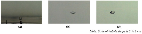
Figure 2.
Three main categories of bubble shape: (a) spherical-cap shape, (b) elliptical shape, and (c) irregular shape.
2.3. Machine Learning Approaches
In general, machine learning can be divided into two major categories, which are supervised and unsupervised learning. The supervised learning method is more widely used, especially in solving the problem related to classification and regression.
2.3.1. Regression Problem-Solving
Feed forward back propagation neural network (FBNN) has great applicability to deal with nonlinear regression problems. For this technique, two processes are involved, which are forward propagation of input data from the input layer through the hidden layer to the output layer and back propagation of error in each layer and constant adjustment of the weight and bias to obtain the optimised outcomes. The mathematical expression of the general concept for feed forward back propagation neural network is described as follows:
Assume refers to the output of the -th neuron in the -th layer of the neural network, then
where x is the input, Y is the output, w is the weight, and b is the bias.
It is an important step to activate the neurons using the transfer function, where the commonly used transfer function is tansig function, as shown in Equation (2):
In this study, FBNN was selected to develop models for the final velocity and drag coefficient prediction of single bubbles, where Re, Eo, and We numbers were chosen as the input features.
Re number is an important dimensionless quantity in fluid mechanics used to predict the flow patterns in different fluid flow situations. It can be defined as the ratio of inertial force to viscous force. The formula of Re number is given as:
where Re is Reynolds number, is density of liquid, is final velocity of bubble, d is diameter of bubble, and is viscous force of bubble. In this case, such a number was fixed in the range of 100 to 3200.
Eo number is another key element in fluid mechanics, particularly while measuring the importance of gravitational forces compared to surface tension and characterizing the single bubble motion. The Eo number can be obtained via:
where Eo is Eotvos number, is gravitational acceleration, is density of liquid, is density of gas phase, and is surface tension. In this study, Eo number ranged from 0.5 to 18.
Meanwhile, We number also plays an important role in fluid mechanics, especially for studying the single bubble motion. It is a measure of the relative importance of the fluid inertia compared to its surface tension. The formula for We number calculation is:
where We is Weber number, is density of liquid, is final velocity of bubble, d is diameter of bubble, and is surface tension. Throughout the experiments, such a value was set within a range of 0 to 16.
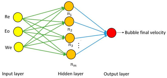
Figure 3.
Architecture for the final velocity prediction model.
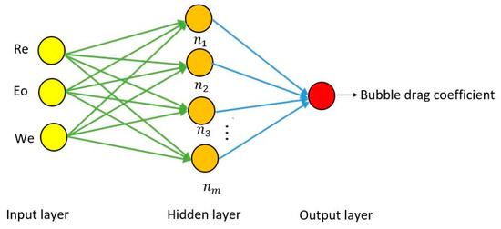
Figure 4.
Architecture for the drag coefficient prediction model.
2.3.2. Classification Problem-Solving
K-nearest neighbours (KNN), random forest, and logistic regression are the common algorithms for classification problem. KNN algorithm achieves the final classification purpose by measuring the distances between the eigenvalues and calculating the difference between the distances. The principle of the KNN algorithm is to find the k distance points closest to the training set and then select the k-nearest neighbours category as its own type. Basically, k is an integer not larger than 20 [33,34]. The basic parameters of the KNN algorithm include distance metrics, k-values, and decision rules of classification.
Entering the dataset X as follows:
where x is the variable and y is the label.
Euclidean distance, as shown in Equation (7), is the generally taken distance:
Meanwhile, the classification law is as follows:
where i = 1, 2, …, N, j = 1, 2, …, K; for the indication function I, when , , otherwise I equal to 0.
On the other hand, the random forest algorithm selects each feature as a classification criterion. The error of the classification depends on the degree of differentiation of each independent feature and the connection among them.
By combining the multiple weak classifiers, the final classification result can be obtained through the voting or averaging method. The weak classifier usually chooses the classification and regression tree (CART) decision tree which uses the Gini index to determine the most appropriate branching feature. The definition is shown in Equation (9):
where pk is the probability of the occurrence of the k-category, the smaller the Gini, the smaller the uncertainty, and the better the data classification.
The CART decision tree avoids the over-fitting through pruning, and the loss function (as shown in Equation (10)):
where C(T) is the error of the trunk T in the training data and a is a trade-off parameter.
Logistic regression algorithm uses the idea of selection probability to classify the sample. In this study, the softmax regression algorithm was chosen to classify the bubble shape. Softmax regression algorithm converts the features into probabilities. The function relationship is as follows:
Meanwhile, the cost function is
where the specific form of I(x) is
Softmax regression algorithm uses the gradient descent method to solve the model parameters. The calculated gradient result is as follows:
All of the above-mentioned algorithms were used to classify the bubble shapes under different dimensionless parameters (Re number, Eo number, and We number). Figure 5 shows the overall flow chart for the machine learning implementation in this study.
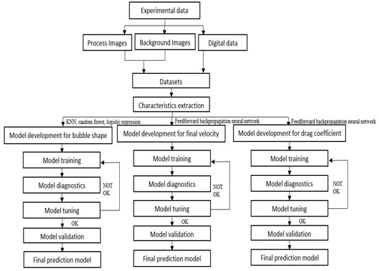
Figure 5.
Process for machine learning implementation.
3. Results
3.1. Prediction Model for the Final Velocity of Single Bubbles
There is a nonlinear yet complex relationship between the final velocity of single bubbles and the dimensionless parameters (Re number, Eo number, and We number). Therefore, a feed forward back propagation neural network (FBNN) was developed to predict the final velocity.
1000 experiment datasets were collected and separated according to the ratio of 70:15:15. 700 datasets were used to train the model, 150 datasets were used for calibration and validation, and the remaining150 datasets were reserved for testing purposes.
While designing the architecture of the model, tansig activation function was selected as the transfer function, while gradient descent was chosen as the optimization method. As shown in Figure 6, the input layer consisted of three nodes (Re number, Eo number, and We number) while the output layer had only one node (final velocity). There were three hidden layers where each of the layers consisted of 10 hidden neurons. In addition, the learning rate was set to 0.01, the number of training was fixed at 1000, and the momentum factor was 0.9. With such a combination of the hyper parameters, the model exhibited good convergence performance during the training process.
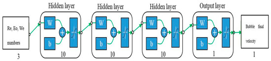
Figure 6.
Architecture of the final velocity prediction model.
Figure 7 and Figure 8 show the model performance in terms of coefficient of determination, R2 for the model validation process, and model testing process respectively, recorded at 0.93 and 0.83. A high R2-value indicates a strong correlation between the actual value and predicted value, where the fitting degree is considerably high.
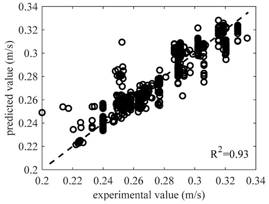
Figure 7.
Plot of the predicted final velocity against the actual final velocity for the validation set.
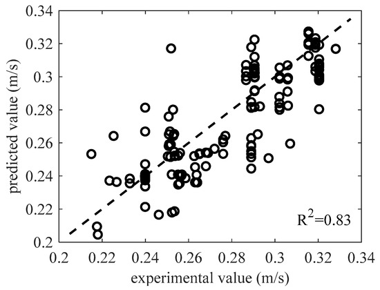
Figure 8.
Plot of the predicted final velocity against the actual final velocity for the testing set.
In order to further verify the appropriateness of the FBNN model, root mean squared error (RMSE) was chosen. A smaller RMSE value indicates a higher level of model accuracy. The equation of RMSE is shown as in Equation (15):
where n is the number of samples, z(x) is the predicted value, and y(x) is the actual value. The calculated RMSE is 0.0741 for the validation set and 0.0518 for the testing set. Such a low RMSE value indicates that the developed model has achieved a relatively good performance. It has the ability to reflect the relationship between the dimensionless number (Re number, Eo number, and We number) and bubble final velocity with a considerably high level of accuracy.
On the other hand, Figure 9 depicted the relationship between R2 and RMSE in both training and testing sets under varying sample size. With the increases of the sample size, the R2 value shows a decreasing trend in training set, but an increasing trend in testing set. Meanwhile, from the perspective of RMSE, such a value decreases gradually in training set but increases gently in testing set when the number of sample increases. Only with the sample size of around 900, the RMSE value for both training and testing set shows an almost similar value, meaning that the model can provide a considerably high level of accuracy with that particular sample size. In other words, it is appropriate to choose a slightly higher sample size of 1000 in this study.
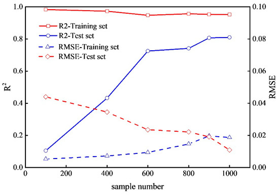
Figure 9.
Relationship between R2 and root mean squared error (RMSE) in both training and testing sets with respect to different number of samples.
3.2. Prediction Model for the Drag Coefficient of Single Bubbles
For bubble drag coefficient prediction model development, the data obtained from experiments were distributed into three portions. Among the datasets, 692 datasets were used for training, 148 datasets were used for validation, while another 148 datasets were kept for testing purpose.
The FBNN model was built with one input layer, three hidden layers, and one output layer, as shown in Figure 10. There were three nodes in the input layer, which are Re number, Eo number, and We number, and only one node in the output, which was bubble drag coefficient. In each hidden layer, there were 10 hidden neurons, and tansig function was selected as the transfer function. By setting the learning rate to 0.001, the number of training to 1000, and the momentum factor to 0.85, the model exhibited good performance during the training process.
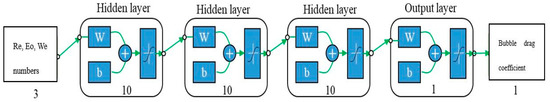
Figure 10.
Architecture of the drag coefficient prediction model.
From Figure 11 and Figure 12, the R2-value for both the validation and testing plot is obviously high, reaching 0.96 and 0.92, respectively. The value is approximate to 1, which indicates that the developed model has achieved a good performance in terms of the coefficient of determination.
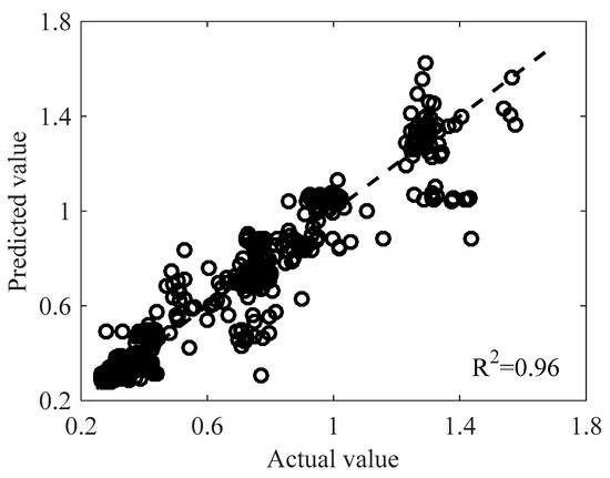
Figure 11.
Plot of the predicted drag coefficient against the actual drag coefficient for the validation set.
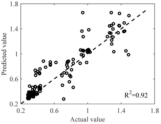
Figure 12.
Plot of the predicted drag coefficient against the actual drag coefficient for the testing set.
In addition, in order to have further verification on the suitability of the model, the RMSE value is calculated. It records at 0.0946 and 0.1534, respectively, for validation set and testing set. Such a low RMSE value indicates that the model is well-performed from the perspective of RMSE.
In order to further show that the developed AI model has the ability to serve as an alternative or replace the need for mathematical calculation, 150 datasets were randomly picked. The predicted values obtained from the model were compared with values calculated through the empirical formulas.
As shown in Figure 13, the drag coefficient (CD) values calculated through the formula as proposed by Tomiyama et al. [35] show a larger deviation from the actual CD values. Meanwhile, the predicted CD values from the developed AI model and calculated CD values from the formula introduced by Dijkhuizen et al. [36] are in good agreement with the actual values.
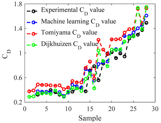
Figure 13.
Comparison of the predicted values from the developed model and empirical formulas from previous researchers with the actual experimental CD values.
From the perspective of the coefficient of determination, the FBNN model exhibits R2 value of 0.9593, while the formulas proposed by Tomiyama [35] and Dijkhuizen [36] show R2 values of 0.9192 and 0.9362, respectively. Also, the RMSE value is calculated for each case, recorded at 0.1291 for the developed FBNN model, 0.2412 for Tomiyama’s formula [35], and 0.1686 for Dijkhuzen’s formula [36].
Based on the above statistical analyses, the predicted value from the developed FBNN model has the highest accuracy if compared with the empirical formulas suggested by the previous researchers.
3.3. Prediction Model for the Shape of Single Bubbles
The number of datasets for learning and testing purposes is 710 and 304, respectively. A platform was built under a Python environment to predict the shape of single bubbles. Three algorithms were applied to perform the task which are KNN, random forest, and logistic regression. The input variables are Re number, Eo number, and We number, while the bubble shapes are labelled with number 1, 2, and 3 to represent the bubbles with elliptical shape, spherical-cap shape, and irregular shape, respectively [37].
Table 2 shows the distribution of the confusion matrix corresponding to the KNN model. Most of the predicted outputs fall accurately and precisely into their own category. In terms of recall rate, the true positive rate (TPR) and true negative rate (TNR) are the two important indicators. TPR value is 76.92% for the elliptical-shaped bubbles, 76.16% for spherical-cap shaped bubbles, and 86.11% for irregular-shaped bubbles. Meanwhile, the TNR value for the bubbles with elliptical shape, spherical-cap shape, and irregular shape is 85%, 76.10%, and 99.25%, respectively. Both the TPR and TNR values for each category are above 75%, indicating that the classifiers of the model perform well. In addition, the Kappa coefficient of the model is 87.55%, showing that the model has a considerably high degree of consistency.
Table 2.
Confusion matrix of the K-nearest neighbours (KNN)algorithm prediction model.
On the other hand, the distribution of confusion matrix for the logistic regression algorithm prediction model is presented in Table 3. Similar to the KNN algorithm prediction model, most of the predicted label falls into its own category accurately. From the point of view of recall rate, the elliptical-shaped bubbles have a TPR of 84.62%, spherical-cap shaped bubbles have a TPR of 87.41%, while irregular-shaped bubbles have a TPR of 94.44%. Meanwhile, for TNR value, it is 90.90% for the bubbles with elliptical shape, 87.5% for the bubbles with spherical-cap shape, and 99.25% for the bubbles with an irregular shape. The TPR and TNR values for all the categories are higher than 80%, indicating that each classifier of the model exhibits good performance. Moreover, the Kappa coefficient of the model is calculated and recorded at 78.28%. As suggested by Cohen [38], such a Kappa coefficient show a substantial agreement between the predicted and actual condition as it falls within the range of 61% to 80%.
Table 3.
Confusion matrix of the logistic regression algorithm prediction model.
The distribution of confusion matrix for the random forest algorithm prediction model is contained in Table 4. The classification through the random forest algorithm displays that most of the predicted data located correctly and accurately in its own category. From the perspective of TPR, it is 87.18%, 86.09%, 83.33%, corresponding to bubbles with elliptical shape, spherical-cap shape, and irregular shape, respectively. Meanwhile, for TNR value, it shows 88.77% for the elliptical-shaped bubbles, 86.27% for spherical-cap shaped bubbles, and 98.16% for the irregular-shaped bubbles. Such high values of TPR and TNR represent that each of the classifiers of the model performs well. For the Kappa coefficient, the calculated value is 76.41%, which indicates that the classification accuracy of the model is substantially high [38].
Table 4.
Confusion matrix of the random forest algorithm prediction model.
Figure 14 shows the sensitivity of each variable in the model developed using the random forest algorithm, where P is the degree of importance. The formula of P is given by:
where is Gini index, m is the number of features, and are Gini index of the two new nodes after branching.
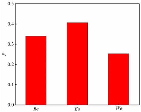
Figure 14.
Degree of importance for each parameter in the random forest prediction model.
Basically, in accordance with the increase of Re, Eo, and We numbers, the bubbles experience a change from elliptical shape to either spherical shape or other irregular shapes. Due to the experimental constraints, only the limited range of the Re, Eo, and We numbers was applied in this study. Nonetheless, the relevant analyses were obtained via bubble phase diagram as proposed by Cliff [37]. In general, the single bubble motion in still water is mainly affected by viscous, gravitational, surface tension, and inertial forces. According to previous studies, the level of significance of different forces exerted on the bubbles varied with the size of bubbles. For instance, surface tension force exhibits the most significant impact on the bubbles with a diameter of less than 6mm, meanwhile, if the size is larger than 6 mm, the bubble is mainly affected by inertial force [1,11,39].
As displayed in Figure 13, the effect of Eo number to the determination of the shape of single bubbles is the most significant, recording at P-value of 0.407. It is followed by Re number with a value of 0.34, and the least significant parameter is We number with a value of 0.253. This is mainly because Eo number is the parameter, which represents the effect of surface tension on motion characteristics of the single bubbles. The finding is in line with [1,11,39], where the diameter of bubbles in this study ranges from 2 to 7.5 mm (mostly below 6mm) and thereby surface tension plays the role as the main force that affects the bubbles. The surface tension is particularly reflected through the dynamic pressure difference. In other words, when the dynamic pressure difference increases, the bubble surface tension changes drastically and complicates the changes of bubble shape.
Figure 15 shows the distribution of bubble shapes with respect to different Re number and Eo number conditions as predicted by KNN, random forest, and logistic regression prediction models. Observing the shape distribution in Figure 15, when Eo falls within the range of 0.5 to 2 and the Re number is in between 600–2000, the bubble is elliptical in shape. When the Eo number ranges from 2 to 5 and the Re number is at a value of 900 to 2000, the bubble is in spherical-cap shape. Meanwhile, when the Eo number falls within the range of 4.5 to 8 and the Re number is recorded at a value of 2000 to 5000, the bubble is irregular in shape.
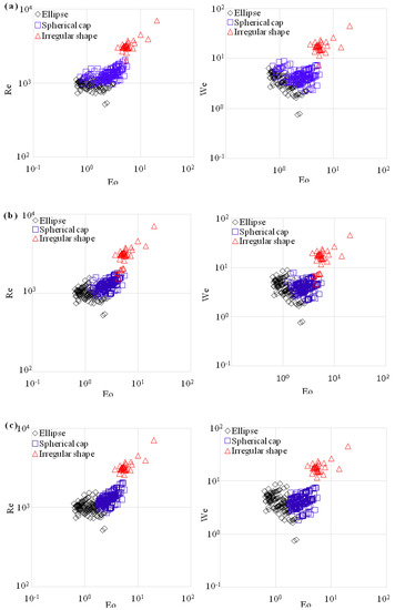
Figure 15.
Distribution of predicted shape of single bubbles under different Re, We, and Eo number with respect to (a) KNN algorithm, (b) random forest algorithm, and (c) logistic regression algorithm.
On the other hand, from Figure 15, it is noticed that, when Eo number is ranged from 0.7 to 2, the prediction results of the KNN algorithm show an overlap scenario. The same phenomenon happens when the Eo number ranges from 1 to 2 for the random forest algorithm.
Overall, based on the discussions under this section, the prediction model developed using logistic regression algorithm has achieved a better performance among the three examined models. Hence, it appears as the most suitable model for the bubble shape prediction.
4. Conclusions
The physical motion of single bubbles in the still water is the main focus of this study, as it plays a significant role in engineering applications, especially for marine engineering.
Since machine learning has been widely used in different fields of study, it is utilised in this research for both regression and classification problem-solving. The major aim of this study is to develop prediction models for the final velocity, drag coefficient, and shape of single bubbles.
For final velocity prediction model development, feed forward back propagation neural network was selected to establish the relationship between the dimensionless parameters (Re number, Eo number, and We number) and bubble final velocity. Such a model has achieved the R2 value of 0.83 and RMSE value of 0.0518, indicating that the model has the ability to predict the bubble final velocity with a considerably high level of accuracy.
While developing the bubble drag coefficient prediction model, the FBNN approach was chosen. The dimensionless parameters (Re number, Eo number, and We number) were kept as the input and the bubble drag coefficient was reserved as the output. The R2 and RMSE value of the model is 0.92 and 0.1534, respectively, meaning that the model has achieved a good prediction performance. It is found that the predicted values from the developed model have a higher accuracy if compared to the values from the empirical formulas proposed by Tomiyama (2002) and Dijkhuizen (2010).
On the other hand, KNN, logistic regression and random forest algorithm were used to develop the prediction model for bubble shape. The performance of each approach was evaluated and the logistic regression prediction model has achieved the best performance.
It is believed that the output models developed in this study can be beneficial to the engineers, scientists, and hydrologists while dealing with the problems related to the motion of single bubbles in still water.
Author Contributions
Conceptualization, B.D. and C.J.; methodology, Y.T.; formal analysis, B.D. and Y.T.; writing—original draft preparation, R.J.C.; writing—review and editing, S.H.L. and R.J.C.; supervision, C.J.; funding acquisition, B.D.
Funding
This research was funded by the National Natural Science Foundation of China, NSFC Grant Nos. 51979015, 51509023, 51839002and 51879015 and Natural Science Foundation of Hunan Province, China, Grant No. 2018JJ3535.
Acknowledgments
The authors would like to thank the School of Hydraulic Engineering, Changsha University of Science and Technology for the facilities provided for their experiments.
Conflicts of Interest
The authors declare no conflict of interest.
References
- Grace, J.R. Shapes and velocities of single drops and bubbles moving freely through immiscible liquids. Chem. Eng. Res. Des. 1976, 54, 167–173. [Google Scholar]
- Terrill, E.J.; Melville, W.K.; Stramski, D. Bubble entrainment by breaking waves and their influence on optical scattering in the upper ocean. J. Geophys. Res. Ocean. 2001, 106, 16815–16823. [Google Scholar] [CrossRef]
- Rayleigh, L. On the pressure developed in a liquid during the collapse of a spherical cavity. Philisophical Mag. 1917, 34, 94–98. [Google Scholar] [CrossRef]
- Mendelson, H.D. The prediction of bubble terminal velocities from wave theory. Aiche J. 1967, 13, 250–253. [Google Scholar] [CrossRef]
- Michaelides, E.E. Particles, Bubbles and Drops: Their Motion, Heat and Mass Transfer; World Scientific Publishing Co. Pte. Ltd.: Singapore, 2006. [Google Scholar]
- Plesset, M.S.; Chapman, R.B. Collapse of initially spherical vapour cavity in the neighbourhood of a solid boundary. J. Fluid Mech. 1971, 47, 283–290. [Google Scholar] [CrossRef]
- VanKrevelen, D.W.; Hoftijzer, P.J. Studies of gas-bubble formation- Calculation of interfacial area in bubble contactors. Chem. Eng. Prog. 1950, 46, 29–35. [Google Scholar]
- Wellek, R.M.; Agrawal, A.K.; Skelland, A.H. Shape of liquid drops moving in liquid media. Aiche J. 1966, 12, 854–862. [Google Scholar] [CrossRef]
- Wu, M.; Gharib, M. Experimental studies on the shape and path of small air bubbles rising in clean water. Phys. Fluids 2002, 14, L49–L52. [Google Scholar] [CrossRef]
- Amaya-Bower, L.; Lee, T. Single bubble rising dynamics for moderate Reynolds number using Lattice Boltzmann Method. Handb. Fluids Motion 2010, 39, 1191–1207. [Google Scholar] [CrossRef]
- Bhaga, D.; Weber, M.E. Bubbles in viscous liquids: Shapes, wakes and velocities. J. Fluid Mech. 2006, 105, 61–85. [Google Scholar] [CrossRef]
- Brücker, C. Structure and dynamics of the wake of bubbles and its relevance for bubble interaction. Phys. Fluids 1999, 11, 1781–1796. [Google Scholar] [CrossRef]
- Funfschilling, D.; Li, H.Z. Flow of non-Newtonian fluids around bubbles: PIV measurements and birefringence visualisation. Chem. Eng. Sci. 2001, 56, 1137–1141. [Google Scholar] [CrossRef]
- Hassan, Y.A.; Ortiza-Villafuerte, J.; Scmidl, W.D. Three-dimensional measurements of single bubble dynamics in a small diameter pipe using stereoscopic particle image velocimetry. Int. J. Multiph. Flow 2001, 27, 817–842. [Google Scholar] [CrossRef]
- Liu, Z.; Zheng, Y. PIV study of bubble rising behaviour. Powder Technol. 2006, 168, 10–20. [Google Scholar] [CrossRef]
- Ortize-Villafuerte, J.; Schmidl, W.D.; Hassan, Y.A. Three-dimensional ptv study of the surrounding flow and wake of a bubble rising in a stagnant liquid. Exp. Fluids 2000, 29, S202–S210. [Google Scholar] [CrossRef]
- Thoroddsen, S.T.; Etoh, T.G.; Takehara, K. High-speed imaging of drops and bubbles. Annu. Rev. Fluid Mech. 2008, 40, 257–285. [Google Scholar] [CrossRef]
- Tokuhiro, A.; Maekawa, M.; Iizuka, K.; Hishida, K.; Maeda, M. Turbulent flow past a bubble and an ellipsoid using shadow-image and PIV techniques. Int. J. Multiph. Flow 1998, 24, 1383–1406. [Google Scholar] [CrossRef]
- Yu, X.; Efe, M.O.; Kaynak, O. A general back propagation algorithm for feed forward neural networks learning. IEEE Trans. Neural Netw. 2002, 12, 251. [Google Scholar]
- Ehteram, M.; Koting, S.B.; Afan, H.A.; Mohd, N.S.; Malek, M.A.; Ahmed, A.N.; El-shafie, A. New evolutionary algorithm for optimizing hydropower generation considering multireservoir systems. Appl. Sci. 2019, 9, 2280. [Google Scholar] [CrossRef]
- Li, X.; Qiu, J.; Shang, Q.; Li, F. Simulation of reservoir sediment flushing of the Three Gorges reservoir using an artificial neural network. Appl. Sci. 2016, 6, 148. [Google Scholar] [CrossRef]
- Bąk, Ł.; Szeląg, B.; Górski, J.; Górska, K. The Impact of catchment characteristics and weather conditions on heavy metal concentrations in stormwater—Data mining approach. Appl. Sci. 2019, 9, 2210. [Google Scholar] [CrossRef]
- Ravansalar, M.; Rajaee, T.; Ergil, M. Prediction of dissolved oxygen in River Calder by noise elimination time series using wavelet transform. J. Exp. Theor. Artif. Intell. 2016, 28, 689–706. [Google Scholar] [CrossRef]
- Deng, Q.; Shao, S.; Fu, L.; Luan, H.; Feng, Z. An integrated design and optimization approach for radial inflow turbines—Part II: Multidisciplinary optimization design. Appl. Sci. 2018, 8, 2030. [Google Scholar] [CrossRef]
- Zhang, Y.; Kim, B. A fully coupled computational fluid dynamics method for analysis of semi-submersible floating offshore wind turbines under wind-wave excitation conditions based on OC5 data. Appl. Sci. 2018, 8, 2314. [Google Scholar] [CrossRef]
- Aghdam, K.M.; Mirzaee, I.; Pourmahmood, N.; Aghababa, M.P. Design of water distribution networks using accelerated momentum particle swarm optimisation technique. J. Exp. Theor. Artif. Intell. 2014, 26, 459–475. [Google Scholar] [CrossRef]
- Vasto-Terrientes, L.D.; Kumar, V.; Chao, T.C.; Valls, A. A decision support system to find the best water allocation strategies in a Mediterranean river basin in future scenarios of global change. J. Exp. Theor. Artif. Intell. 2016, 28, 331–350. [Google Scholar] [CrossRef]
- Goldstein, E.B.; Coco, G. A machine learning approach for the prediction of settling velocity. Water Resour. Res. 2014, 50, 3595–3601. [Google Scholar] [CrossRef]
- Chang, F.-J. Artificial intelligence for integrated water resources management in Taiwan. J. Water Resour. Res. 2013, 2, 316–322. [Google Scholar]
- Chang, F.-J.; Tsai, W.-P.; Cheng, C.-L. Intelligent water resources management strategy under urbanisation. J. Water Resour. Res. 2016, 5, 314–325. [Google Scholar]
- Chin, R.J.; Lai, S.H.; Shaliza, I.; Wan Zurina, W.J.; Elshafie, A. Rheological wall slip velocity prediction model based on artificial neural network. J. Exp. Theor. Artif. Intell. 2019, 659–676. [Google Scholar] [CrossRef]
- Chin, R.J.; Lai, S.H.; Shaliza, I.; Wan Zurina, W.J.; Elshafie, A.H. New approach to mimic rheological actual shear rate under wall slip condition. Eng. Comput. 2018, 35, 1–10. [Google Scholar] [CrossRef]
- Brackhill, J.U.; Kothe, D.B.; Zemach, C. A continuum method for modelling surface tension. J. Comput. Phys. 1992, 100, 335–354. [Google Scholar] [CrossRef]
- Samkhaniani, N.; Ansari, M.R. Numerical simulation of bubble condensation using CF-VOF. Prog. Nucl. Energy 2016, 89, 120–131. [Google Scholar] [CrossRef]
- Tomiyama, A.; Celta, G.P.; Hosokawa, S.; Yoshida, S. Terminal velocity of single bubbles in surface tension force dominant regime. Int. J. Multiph. Flow 2002, 28, 1497–1519. [Google Scholar] [CrossRef]
- Dijkhuizen, W.; Annaland, M.V.; Kuiper, J.A. Numerical and experimental investigation of the lift force on single bubbles. Chem. Eng. Sci. 2010, 65, 1274–1287. [Google Scholar] [CrossRef]
- Cliff, R.; Grace, J.R.; Weber, M.E. Bubbles, Drops, and Particles; Dover Publications Inc: New York, NY, USA, 2005. [Google Scholar]
- Cohen, J. A coefficient of agreement for nominal scale. Educ. Psychol. Meas. 1960, 20, 37–46. [Google Scholar] [CrossRef]
- Grace, J.R. Hydrodynamics of liquid drops in immiscible liquids. Handb. Fluids Motion 1983, 38, 273. [Google Scholar]
© 2019 by the authors. Licensee MDPI, Basel, Switzerland. This article is an open access article distributed under the terms and conditions of the Creative Commons Attribution (CC BY) license (http://creativecommons.org/licenses/by/4.0/).