Abstract
With a rising demand for utilizing unmanned aerial vehicles (UAVs) to deliver materials in outdoor environments, particular attention must be given to all the different aspects influencing the deployment of UAVs for such purposes. These aspects include the characteristics of the UAV fleet (e.g., size of fleet, UAV specifications and capabilities), the energy consumption (highly affected by weather conditions and payload) and the characteristics of the network and customer locations. All these aspects must be taken into account when aiming to achieve deliveries to customers in a safe and timely manner. However, at present, there is a lack of decision support tools and methods for mission planners that consider all these influencing aspects together. To bridge this gap, this paper presents a decomposed solution approach, which provides decision support for UAVs’ fleet mission planning. The proposed approach assists flight mission planners in aerospace companies to select and evaluate different mission scenarios, for which flight-mission plans are obtained for a given fleet of UAVs, while guaranteeing delivery according to customer requirements in a given time horizon. Mission plans are analyzed from multiple perspectives including different weather conditions (wind speed and direction), payload capacities of UAVs, energy capacities of UAVs, fleet sizes, the number of customers visited by a UAV on a mission and delivery performance. The proposed decision support-driven declarative model supports the selection of the UAV mission planning scenarios subject to variations on all these configurations of the UAV system and variations in the weather conditions. The computer simulation based experimental results, provides evidence of the applicability and relevance of the proposed method. This ultimately contributes as a prototype of a decision support system of UAVs fleet-mission planning, able to determine whether is it possible to find a flight-mission plan for a given fleet of UAVs guaranteeing customer satisfaction under the given conditions. The mission plans are created in such a manner that they are suitable to be sent to Air Traffic Control for flight approval.
1. Introduction
The immense development of unmanned aerial vehicle (UAV) capabilities has promulgated its influence in many domains, such as defense, search and rescue, agriculture, manufacturing, and environmental surveillance [1,2,3,4] to execute complex industrial functions. Fleet-mission planning for UAVs in the context of materials delivery has become a major research topic [5,6,7,8] and could be treated as an extension of the vehicle routing problem (VRP) [9] which belongs to the class of planning problems that are NP-hard [10,11]. Various objectives could be used in UAV mission planning such as reducing individual UAV costs, enhancing its profit, increasing safety in operations, reducing lead time, or increasing the load capacity of the entire system [12,13]. UAV routing in 3-D environments has different degrees of attractiveness when evaluated against multiple decision criteria, which relates to finding the sequence of waypoints that connects the start to the destination locations [14,15,16,17]. Existing studies on UAV routing for transporting materials and surveillance [9] have given less attention to changing weather conditions and the non-linear fuel consumption behaviors of UAVs [18].
This study addresses the problems of routing and scheduling of a UAV fleet, considering the changing weather conditions. The focus of the study is the solutions that allow for finding feasible, collision-free flight plans ensuring non-empty batteries for a fleet of UAVs. This approach maximizes the satisfaction of the orders from given customers. The proposed declarative solution approach enables one to state a decision support-driven reference model aimed at the analysis of the relationships between the structure of a given UAV-driven supply network and its potential behavior, resulting in a sequence of sub-missions following required deliveries. From this perspective, the results of this study fall within the scope of the research presented in the papers [19,20,21,22,23,24].
Numerous parameters and constraints influence the decision criteria for UAV fleet mission planning. Typical limitations of UAVs in transportation systems include the limited flight range, which depends on the battery capacity, the payload of the UAV, overlapping air corridors designated for UAV movement and the technical specifications of UAVs [8]. Furthermore, the decision space consists of aspects which include routing and scheduling in the 3-D environment, the carrying payload of the UAVs and collision avoidance with moving or fixed objects, energy consumption affected by the changing conditions like wind speed, wind direction and air density [8].
Thus, these various interdependent aspects emphasize the intractability of UAV fleet-mission planning because it is challenging to develop models considering all the influencing aspects together. There is little knowledge on how the changes in these influencing parameters affect the solutions, even concerning deterministic approaches. For instance, the collision avoidance solutions differ regarding fixed obstacles vs. moving flying obstacles and single obstacles vs. many obstacles. Studies in the literature have used methods for UAV mission planning where the routes have been derived by satisfying the UAV dynamics using linear approximations for energy-consumption models [25,26]. Certain existing models have not considered all the significant physical properties related to UAVs and have used approaches such as VRP with time windows (VRPTW) [27,28].
Depending on the context of the problem, mission planning can be done online or offline. Most of the online mission planning has been done assuming that the UAVs can detect the obstacles using sensors to avoid collisions [29]. Because of the recent advances in collision-avoidance technology, most small UAVs can sense the air traffic and alter flight altitudes or turn to avoid collisions. Studies regarding routing problems in communication networks do not explicitly avoid collisions between UAVs [11]. Because this study does not consider small UAVs, such assumptions are not valid, and the study has to create offline mission plans with flight plans for each UAV where it needs to be sent to the authorities in advance to get the approval to be executed afterward. In offline planning, collision avoidance could be done by predicting potential collisions where online planning reacting strategies are utilized.
Moreover, the techniques to avoid collision change when the fleet of UAVs are flying in free space vs. dedicated corridors. Depending on the context of the problem, different strategies have to be adopted for collision avoidance [30]. This study focuses on offline mission planning of UAVs by predicting the collisions in advance and planning missions ensuring collision avoidance, where the principle of prevention is used as a guarantee of UAV deadlock-freeness.
The payload capacity and the flight range of the UAVs are related to the energy capacity, and these aspects are vital in mission planning [31,32]. Studies have proposed to segregate the whole network area considering the UAVs’ relative capabilities and proposed clusters in the area to reduce the problem size [33,34,35,36]. In this study, customer nodes are clustered to reduce the complexity of the network, where each cluster has a set of feasible UAVs fleet routings, and accompanying schedules are provided.
Weather conditions are pertinent to UAV routing because wind speed and wind direction could agitate the travel speed of the UAV, and the air density, appeased by the temperature in the atmosphere, affects the energy consumption in UAVs [9] where cold temperatures may adversely affect battery performance [9]. The majority of the current state of research has paid less attention to weather factors and ignores the impact of weather on performance [14,33,37]. The current literature has sporadically considered wind conditions on energy consumption and the use of that information in planning the missions [9,38,39]. The studies have assumed constant wind speed and direction [38] and have used linear approximations for energy consumption, giving less focus on the impact of weather [9]. Because of the UAVs used in this study, linear approximations are not coherent. The weight of the UAVs used here are heavier than the UAVs used in existing research because the studies have stated that their models are not reasonable when the weight of UAVs increases [9]. Accordingly, the non-linear models proposed in the literature are used in this study in calculating energy consumption considering weather conditions [24].
The mission-planning problems addressed in this study cover different layers of system architecture, which include fleet level where the fleet is managed to provide delivery service and the platform level where it focuses on the individual functioning of the UAVs. Thus, the contributions of this study cover both fleet and platform levels as shown in Figure 1. The goal of this study is to fill the gap in literature addressing UAV fleet-mission planning in changing weather conditions, maximizing customer demand satisfaction in a given time period. Because of the novelty of the problem and the fact it covers different layers of decisions, the initial objective of this study is to find a reasonable way to solve the problem. It is difficult to claim that any proposed method is the best way to solve a problem, but this method allows future research to find better approaches to solve the problem.
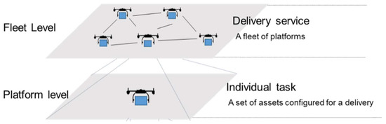
Figure 1.
Overall hierarchical representation of the system related to the problem.
The remainder of the paper is organized as follows: Section 2 provides the problem formulation and the composition of the central problem concerning UAV fleet-mission planning with changing weather conditions. Section 3 presents models for the problem of UAV mission planning. Then, the already stated problem formulated with a declarative solution approach aimed at addressing problem composition is considered in Section 4 An illustrative example of the proposed approach is discussed in Section 5, and the concluding remarks are presented in Section 6.
2. Problem Formulation
The central problem addressed in this study focuses that a given set of customers at different points is to be served during a time period, which consists of changing weather conditions by a fleet of UAVs.
The main problem boils down to the general question of: Is it possible to find a sequence of UAV missions (termed as sub-missions) which contain routes; schedules and an amount of transported materials () of a given UAV fleet, which maximize the customer demand fulfilment under changing weather conditions, while considering energy limits of UAVs and ensuring collision avoidance?
As mentioned in the literature analysis presented, there are still no effective solutions which allow operators to plan the routes and schedules for a fleet of UAVs under changing weather conditions. In order to find a solution, the problem is deconstructed into four sub-problems, where each sub-problem helps to reduce the complexity of the main problem.
2.1. Determining the Sub-Mission Time Windows
In order to reduce the complexity of the weather conditions in the main problem, the first sub-problem considered assumes that a given time period with changing weather conditions is to be divided into several sub-mission time windows (STWs). The STWs consist of analogous weather conditions. The goal is to determine the length of STWs and create a sequence of STWs, such that each window consists of a range of wind speed and a wind direction.
The weather forecast is constant for the assumed time period, and the weather data is used to determine the STWs, in which the weather conditions are held constant, such as the speed and direction of the wind. The minimum and maximum ranges of wind speed for each sub-mission time window are known in advance. The wind direction is the same inside any given sub-mission time window. The sub-mission time windows can be subdivided into flying-time windows (FTWs) assuming that a given time duration with similar weather conditions is to be divided into several flying time windows. The intention is to determine the length of FTWs depending on the time used in the flying of UAVs, considering the maximum energy limit and maximum carrying payload.
The UAV airspeed is the speed of a UAV relative to the air. Because the UAV needs to maintain a constant ground speed, the UAV needs to adjust its airspeed to fly in the desired flight path. Each sub-mission time window consists of a minimum and a maximum range of wind speed and a specific wind direction. This information leads to a min and max range of airspeed because of the effect of the wind speed and direction. Using the min and max range of air speed, the range of energy consumption is calculated. Every travelled route of a UAV starts and finishes within a given FTW. All UAVs are filled with full energy capacity before they start to fly and one UAV can fly only one time during the FTW. Each UAV has enough energy capacity to travel directly to the farthest customer in the network and come back directly to the depot in the worst acceptable weather conditions. The results of this sub-problem provide a sequence of STWs where the time period is divided into several STWs where each STW is divided into FTWs.
2.2. Determining the Clusters of Customers
In order to reduce the complexity of the network and the customer demand requirements in the main problem, the second sub-problem considered assumes that a given set of customers at different points will be grouped into customer clusters (CL). These customers in the cluster can be served by UAVs considering the maximum energy limit. The claim is to create alternative clusters for each flying-time window, such that customers in each cluster could be served by UAVs to deliver a portion of customer demand. The output of this sub-problem provide a set of alternative clusters of customers for each flying-time window.
2.3. Creating a Possible Set of Sub-Missions
In order to reduce the complexity in the scheduling and routing of UAVs, the third sub-problem considered assumes that a given set of customers in a cluster will be served during a given flying-time window. The flying-time windows consist of a set of sub-missions, such that each sub-mission consists of routes with schedules of the UAVs delivering materials to the customers. The goal is to create a set of sub-missions for each cluster, such that the customers in the cluster are reached with a portion of the demand during each flying-time window while obeying the energy constraints and assuring collision avoidance.
This study assumes that more than one UAV can start to fly from the base at the same time and that all UAVs fly at the same altitude. The amount of weight allocated to the customers in a route is an integer where similar kinds of material are delivered to customers in differing amounts [Kg] and customers can accept deliveries during the time period. The output of this sub-problem provide a possible set of sub-missions for each cluster of customers for each flying-time window.
2.4. Finding Sequences of Sub-Mission Deliveries which Give the Maximum Customer Satisfaction
In order to reduce the complexity in the main problem, the fourth sub problem considered assumes a given set of customers is to be served during a time period at different points by a planned mission using a fleet of UAVs, which consist of a sequence of sub-missions. The goal is to find admissible missions which maximize the customer demand fulfilment, such that the sum of the sub-mission deliveries provide maximum demand fulfilment. A secondary objective is to find the admissible solutions with minimized total time travelled/total energy consumed. The output of this sub-problem provide a sequence of sub-missions, which maximize customer demand fulfilment.
2.5. Interdependency between Sub-Problems
Figure 2 shows the relationships between the sub-problems based on the influences from the outputs of each sub-problem. The interdependencies between the sub-problems, illustrated in Figure 2, are as follows.
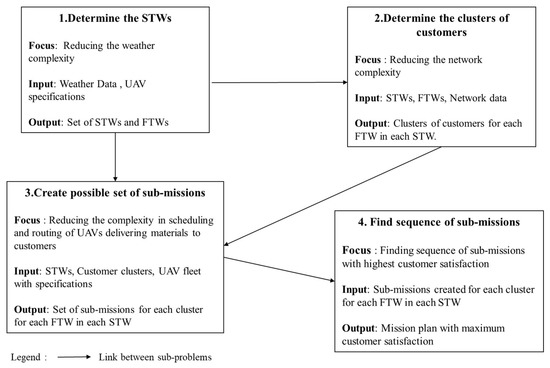
Figure 2.
Interdependency between the decomposed sub-problems.
Sub-problem 1 to sub-problem 2: for each STW, a set of selected clusters of customers in the network are considered to plan the delivery missions. Sub-problem 2 to sub-problem 3: for each customer cluster, a set of feasible collision-free UAV routings and accompanying schedules are created. Sub-problem 1 to sub-problem 3: each sub-mission is created inside a given STW where the range of wind speeds and direction is known. The creation of sub-missions is influenced by the nature of weather condition in each STW. Sub-problem 3 to sub-problem 4: the sequence of sub-missions from each FTW provides a full mission. The sub-missions created in sub-problem three are searched to find the sequence which provides the maximum customer satisfaction.
As we consider the whole problem with the constraints and the system requirements, a general approach has to be designed to deliver feasible output addressing the whole problem with an overall quality solution. If each sub-problem is focused on individually, better different alternatives could be found but when all the sub-problems are considered together because of the interdependency between the sub-problems a general approach is proposed. An interdependency analysis substantiates that sub-problem 3 is the most difficult problem to focus on because all of the rest of the sub problems are linked with it. Moreover, sub-problem 3 has the most generic aspects to focus on. Hence this paper focuses more on sub-problem 3.
The mathematical formulation of the model considered employs the following symbols explained in Table 1.

Table 1.
Notation table.
3. Problem Modeling
The concept of the considered problem is illustrated in Figure 3. In this illustrative example, a set of customers located at different points in a delivery distribution network are to be serviced by a fleet of UAVs during a specified time period in which changing weather conditions are encountered. Figure 3 illustrates the time period as a sequence of STWs, which consists of different weather conditions. Each STW consists of a range of wind speed and a given wind direction so that in the creation of routes and schedules for the UAV fleet, the weather data of each STW are considered. The specifications of the UAVs, network data with flying corridors and customer locations, customer demands and weather conditions are given as input data. A solution strategy should be used to create a final mission plan, which consists of a sequence of sub-missions, which consists of routes and schedules (orange and blue lines) for the UAVs fleet as shown in the latter part of Figure 3. The objective function and the constraints are as specified below.
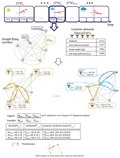
Figure 3.
Problem modeling illustration.
The objective function
The objective is to maximize the customer satisfaction levels for all the customers by delivering as much as demanded as possible.
The constraints
Arrival time at nodes: Relationship between and .
If an edge is utilized by UAV in a given flying-time window then the arrival time to node is equal to the sum of travel time between node to , time spent for take up landing and the arrival time to node (2).
Collision avoidance: When two edges are crossing (), UAVs occupied in those two edges ( and ) must not be occupied at the same time.
Capacity: The demand assigned to a UAV should not exceed its capacity.
Sum of all the carried weights by UAV should not exceed the maximum carrying payload .
The flow of UAVs: When a UAV arrives at a node that UAV must leave from that node.
The sum of all the occupied edges which goes to node () should be equal to the sum of all the edges which leave from node ().
Start and end of routes: Each UAV that departs from the depot (Node 0) should come back to the depot.
Constraint (6) make sure that each UAV departs from the depot and comes back to the depot. The sum of all the edges which starts from depot and sum of all the edges which returns to depot should be equal to one.
Energy: Each UAV has a maximum energy capacity of Pmax, and in flight, it is not possible to consume more than the max energy capacity.
where is the aerodynamic drag coefficient, A is the front facing area, is the empty weight of the UAV, D is the density of the air, b is the width of the UAV and g is gravitational acceleration (A. Thibbotuwawa et al. 2020). The air speed of a UAV is defined in the following way:
The main question for this study to focus on is: is it possible to find a sequence of UAVs’ sub-missions, (which are determined by decision variables: , , , ) of given UAV fleet, which maximize the customer satisfaction (1) (customer demand (Di) fulfilment) under changing weather conditions considering energy constraints of UAVs (7), ensuring collision avoidance (3), and satisfying the constraints (2),(4)-(6))?
4. Declarative Solution Approach
In order to solve the main problem by addressing the deconstructed sub-problems stated in Section 2 and depending on the link between the sub-problems, either a sequential approach or a parallel approach can be used [40]. In this study, a sequential approach is proposed, which is illustrated in Figure 4.
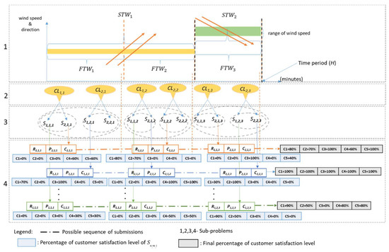
Figure 4.
Proposed solution approach.
4.1. The Method to Determine the Sub-Mission Time Windows
Given the variable about the weather: data about weather forecast in the time period
Question: How many sub-mission time windows should be extracted in the time period and how many flying time windows should be extracted in each sub-mission time window? What are the values of variables determining the STWs: , ?
By using the weather forecast data, the possible length of STWs are determined by using the following steps.
Step 1: Take the forecast data for the planning time period.
Step 2: For each consecutive R hours of sliding time windows, calculate the weather utility value (WUV). R is a parameter with a range of [1,3]. = α (standard deviation of the wind direction) + β (standard deviation the wind speeds). α and β are the weighted parameters.
Step 3: Sort the sliding time windows in ascending order of . Select the time windows based on the weather utility value and divide the time period into different sub-mission time windows.
The method mentioned above creates a sequence of STWs where the time period is divided into several STWs. The purpose is to create sub-missions during a time where there are similar weather conditions. Based on the traveling time of the UAV, assuming that it is flying against the wind and considering the maximum energy limit, the flying-time windows are determined. The STWs are divided in flying-time windows based on the time used in flying the UAVs considering the maximum fuel limit and maximum carrying payload.
4.2. The Method to Determine the Clusters of Customers
The given variables are , , ,
Question: How do we determine clusters of customers which should be extracted from the transportation network in each flying time window?
Determining the number of customers to be put in the cluster can be achieved in several ways such as hierarchical clustering and expectation–maximization clustering and “k-means” clustering. The “k-means” clustering algorithm is selected to do the clustering because it is less time consuming and it is already used in existing literature [36,41]. Customer locations are taken as the feature of the clustering algorithm.
4.3. The Method to Create a Possible Set of Sub-Missions
Given are l-th flying time window: , , , ,,
Question: Does a set of admissible sub-missions satisfying the energy constraints and collision avoidance exist?
The method of creating a possible set of sub-missions for a cluster in a given flying time window has two stages as shown in Figure 5. Stage one creates a list of scenarios for the cluster and stage two creates sub-missions using the scenarios made in stage one.
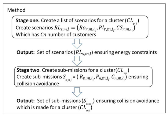
Figure 5.
Illustration of the method to create sub-missions for each mth cluster in each lth flying-time window (FTW).
Stage one and stage two is executed for each cluster for each FTW. The sub-missions are created for each mth cluster in each lth FTW. This calculation provides a set of sub-missions for each cluster in each time window. All the sub-missions in all clusters in a flying-time window equal to the total number of sub-missions made for that flying time window. As the output, it provides sets of sub-missions for each flying time window. is calculated assuming that UAV travels with maximum payload using (6).
Stage one: Create possible scenarios , which consist of routes with schedules and levels of customer satisfaction for a cluster in a FTW. Scenarios consist of a number of customers and each customer receives a portion of materials which is equal to the payload of the UAV divided by . is a parameter with the range of [1, max number of customers in the cluster]. Scenarios are created which have one customer to a maximum number of customers in the cluster. The desired number of scenarios are given as the input in this method and the method stops when, the list of scenarios (RL) consists of the desired number of scenarios.
Stage two: Input for stage two is the list scenarios (RL) for routes with plans and customer satisfaction levels made in stage one for a cluster. The sub-missions for each cluster are created as per the method shown in Figure 6 and Figure 7. The elements are explained below.
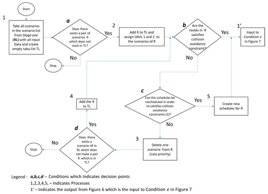
Figure 6.
The heuristic to create sub-missions with collision avoidance for a cluster in an FTW.
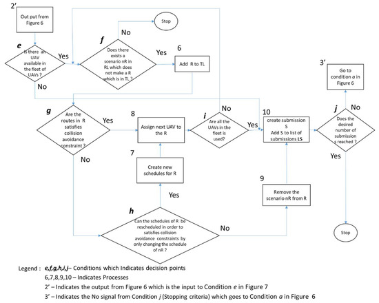
Figure 7.
The heuristic to create sub-missions with collision avoidance for a cluster in an FTW.
Step 1 takes all scenarios in the scenario list (RL) as input data, which comes from stage one, and move to condition a. Input data includes the UAV fleet size, priority of UAVs and the desired number of sub-missions. An empty tab list (TL) is created in this step to store the pairs of scenarios.
Condition a checks whether a pair of scenarios exist in R which do not exist in TL. If yes, it moves to step 2 and, if not, it moves to step 3.
Step 2 adds R to TL and assign the UAVs to R. Then it moves to condition b.
Condition b checks whether the routes in R satisfies the collision avoidance constraint (2). If yes, it moves to step 1’ (which goes as an input to condition e in Figure 7) and, if no, it moves to condition c. Condition c checks whether schedules of R can be rescheduled in order to satisfy collision avoidance constraints (2). If yes it moves to step 6 and if not, it moves to step 4.
Step 3 deletes one scenario assigned to the UAV with less priority from R and moves to condition d. Condition d checks whether there exists a scenario nR in RL, which does not make a pair R which is already in TL. If no, it stops the process and, if yes, it moves to step 5.
Step 4 adds R to TL and moves to condition b.
Step 5 creates new schedules for R and move to step 1’ (which goes as an input to condition e in Figure 7).
Step 2’ takes the output from Figure 6 and moves to condition e where it checks whether there exists an available UAV in the fleet of UAVs. If yes, it moves to condition f and if not, it moves to step 10. Condition f checks if there exists a scenario nR in RL which does not make an R which is in TL. If no, it stops the process and if yes, it moves to step 6.
Step 6 adds the created R to TL. Then moves to condition g.
Condition g checks whether the routes in R satisfies the collision avoidance constraint (2). If yes, it moves to step 8 and if not, it moves to condition h.
Condition h checks whether the schedules of R can be rescheduled in order to satisfy the collision avoidance constraints by only changing the schedule of nR. If yes, it moves to step 7 and if not, it moves to step 9.
Step 7 creates new schedules for R and moves to step 9.
Step 8 assigns next UAV to R moves to condition i.
Step 9 removes the scenario nR from R and moves to step 10. Condition i checks whether all the UAVs in the fleet are used. If yes, it moves to step 10, and, if not, it moves to condition f.
Step 10 creates the sub-missions (Sn,m,l) and adds to the list of sub-missions LS. Customer satisfaction levels of a customer in a sub-mission are equal to the total of customer satisfaction levels of that customer in all the routes in that sub-mission. Then it moves to condition j.
Condition j checks whether the desired number of sub-missions are reached. If yes, it stops the process and, if not, it moves to step 3’ (which goes as an input to condition a in Figure 6). The output of this algorithm provides a possible set of sub-missions.
Stage one and Stage two should be executed for each cluster in the flying-time window. This approach provides a set of sub-missions for each cluster in each flying-time window. Sum of all the sub-missions in all clusters in a flying-time window equals to the total number of sub-missions made for that flying-time window. As the output of the solution in it provides sets of sub-missions for each flying-time window.
4.4. The Method to Find Sequences of Sub-Mission Deliveries, Which Give the Maximum Customer Satisfaction
Given data are: a set of flying-time windows: , , set of clusters and the set of admissible sub-missions for each cluster in each flying-time window.
Question: How to find the sequence of sub-mission deliveries that maximize the customer demand fulfilment?
All sets of possible sequences of sub-missions are searched using brute-force search for small instances where networks, having less than 15 customer nodes. For large instances, the depth-first iterative-deepening (DFID) algorithm is proposed to find admissible missions which gives the highest customer satisfaction because it does not have the drawbacks of most of the other searching algorithms [42,43]. Since DFID expands all nodes to a given depth before expanding any nodes to a greater depth, it is guaranteed to find an asymptotically optimal solution [42].
5. Numerical Example, Results and Discussion
5.1. Numerical Example and Results
The objective of the study is to find an admissible sequence of sub-missions where customer satisfaction is maximized by the end of the time period. Based on the approach for the proposed solution it can be seen that the creation of sub-missions is the most critical element because of the interdependency analysis of the sub-problems. Hence, in this section, the method for the proposed solution for sub-problem 3 is tested using numerical examples to observe the changes in the output for the different inputs for the parameters shown in Table 2. All experiments were performed with a fleet of UAVs having the characteristics mentioned in Figure 2. The STWs considered consist of different lengths where the STW are the outputs of step 1 of the solution.
Table 2.
Input data for the experiments.
For each FTW which falls under a STW, the input parameters for the UAV fleet size, maximum carrying payload, the number of customers per route and the maximum energy of the UAV are changed to make the sub-missions while all remaining parameters are kept constant. Weather data are taken from the actual and forecast weather data from Denmark from 2006 to 2016. Distance data is taken from the network shown in Figure 8. All experiments were implemented in Java using Netbeans IDE 8.2 (Apache Software Foundation, Oracle Corporation, Las Vegas, USA) and conducted on a personal computer with a 2.7 GHz processor and 8 Gb RAM.
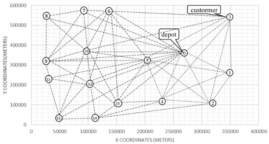
Figure 8.
Map with customer locations and network.
By using the input data, sub-missions are created for each cluster for each flying time window. The creation of sub-missions is done by the method proposed in Figure 5. The example of a cluster containing five customers (1–5) and an FTW of 20 minutes is considered here to illustrate the creation of sub-missions (Figure 9, Figure 10, Figure 11 and Figure 12).
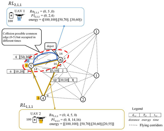
Figure 9.
Scenarios assigned to UAVs, which have routes with common edge occupied at different times.
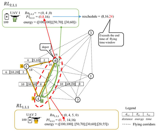
Figure 10.
Scenarios assigned to UAVs with collisions, which are not possible to reschedule.
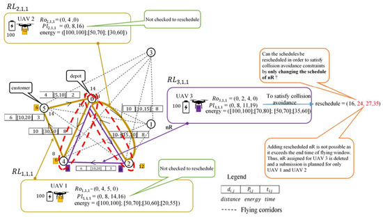
Figure 11.
Checking the condition h for UAVs by rescheduling the only nR.
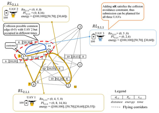
Figure 12.
An illustration showing that adding nR satisfies the collision avoidance constraint.
For possible sub-missions, which contain a different number of customers per route, the average total distance travelled by a sub-mission concerning a different size of the fleet is shown in Figure 13.
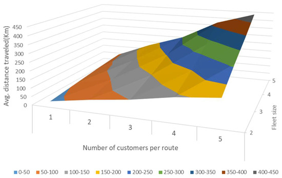
Figure 13.
Average total distance travelled in km when the number of customers per route and fleet size is changing for sub-missions.
The length of the FTWs regarding the changes in the number of customers per route and the UAV fleet size is shown in Figure 14. This data can be used to determine the parameters of fleet size and the number of customers per route in different lengths of FTWs. Depending on the length of the FTWs, sub-missions having different parameters for fleet size and number of customers per route can be used to deliver materials to customers.
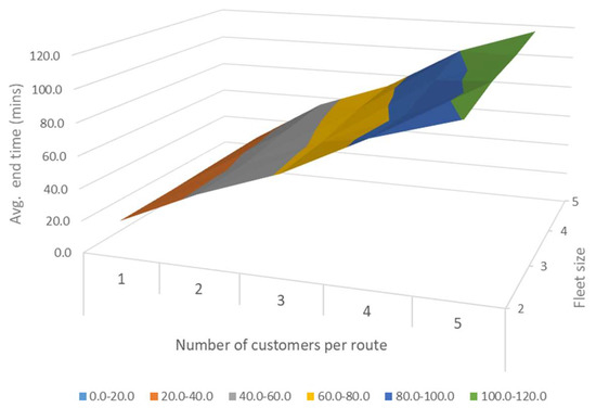
Figure 14.
The average end time of sub-missions in minutes when the number of customers per route and fleet size is changing for sub-missions.
Customer satisfaction levels are shown in Figure 15 for different wind speeds (m/s) for sub-missions having different fleet sizes and numbers of customers per route. (Cn- number of customers per route, K-fleet size). It shows that depending on the wind speed, the number of materials which can be delivered to customers is changing for the sub-missions, which consist of various combinations of fleet size and numbers of customers per route.
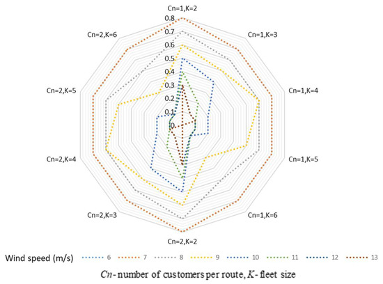
Figure 15.
Customer satisfaction levels for the sub-missions created at different wind speeds.
The customer satisfaction levels are shown in Figure 16 for different wind directions for sub-missions having different fleet sizes and numbers of customers per route. It shows how the different combinations of fleet sizes and numbers of customers per route are changing regarding the changes in wind direction for a given wind speed. These results can be used to choose the parameters for sub-missions depending on the weather conditions in the FTW.
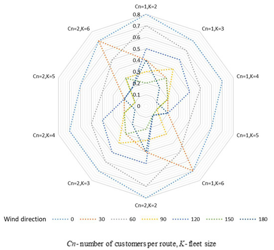
Figure 16.
Customer satisfaction levels for the sub-missions created for different wind directions and with different combinations of fleet size and numbers of customers per route.
The length of the FTWs regarding the changes in the number of customers per route and the UAV fleet size without putting the collision avoidance constraint is shown in Figure 17. This data can be used to analyze the increased percentage of the length of FTWs in comparison with the scenarios where the collision avoidance constraints are considered.
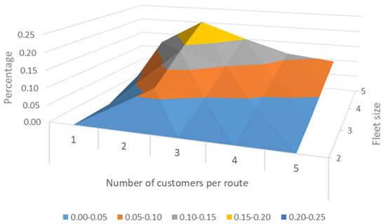
Figure 17.
The increased percentage of length of FTWs because of collision avoidance.
The obtained flight mission for the first, second and last FTWs are shown in Figure 18, Figure 19 and Figure 20. The colored lines (blue line, orange line and purple line) are corresponding to the routes of the UAVs and the customers’ satisfaction levels are shown for each FTW where by the last FTW it shows that all the customers are fully satisfied by the output.
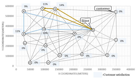
Figure 18.
Obtained flight-mission plan for the first FTW.
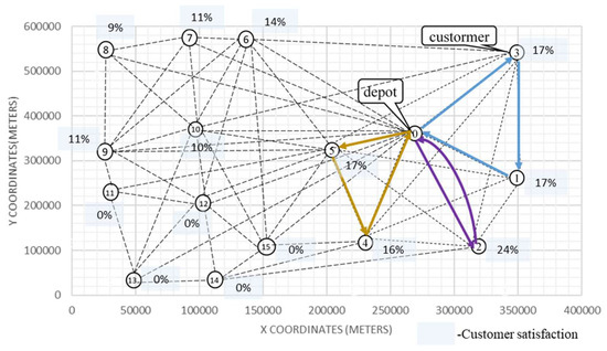
Figure 19.
Obtained flight-mission plan for the second FTW.
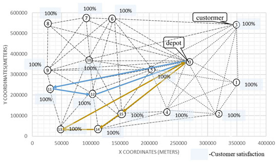
Figure 20.
Obtained flight-mission plan for the last FTW.
Based on the experiment results, sub-missions having different combinations of fleet size and numbers of customers per route could be used to deliver similar amounts of customer demands. However, depending on the length of FTWs different sub-missions can be chosen to execute the missions. It is observed that the collision avoidance constraint increases the flying time of the sub-missions and if a different network can be used where there is less crossing between flying corridors, then the flying time of sub-missions will be reduced, compared to the current network. Hence, the nature of the network influences the results of the creation of sub-missions. Based on the results shown in Figure 14, the sub-missions having different parameters for fleet size and numbers of customers per route can be used to deliver materials to the customers, depending on the length of FTWs. Figure 16 and Figure 17 indicate that different combinations of fleet size and numbers of customers per route are changing concerning the changes in wind direction and wind speed. These results can be used to choose the parameters for sub-missions depending on the weather conditions in the FTW.
5.2. Discussion
Previous studies have first formulated the mission planning problem for a fleet of UAVs as a mixed-integer non-linear programming problem, but subsequently approximated it as a mixed-integer linear programming problem and used Gurobi (Version 6.2, Gurobi GmbH, Berlin, Germany) for solving this formulation of the problem [44,45]. Fügenschuh and Müllenstedt [44] consider energy limitations of UAVs, but do not consider the effects of weather conditions in deriving the energy consumptions and used linear approximations of the energy consumption of UAVs. In the study presented in this paper, linear approximations were not used and weather conditions were considered when calculating the energy consumption of UAVs. Furthermore, in Radzki et al. [46] the problem is formulated as an extension of the VRPTW and is solved in a constraint-programming environment (IBM ILOG). Such programming environments could only provide solutions for relatively small networks in which the number of UAVs are lower than or equal to 4, and the number of customers is lower than or equal to 8 [46]. Thus, in contrast to the existing literature this study proposes the first declarative model for the UAV fleet-mission planning problem, which enables decision support for UAVs’ fleet-mission planning considering all the influencing aspects together. These aspects include characteristics of UAVs fleet, characteristics of energy consumption affected by the weather conditions, characteristics of the network and customer locations. Furthermore, the weight of the UAVs used here exceed these used in existing research (this study uses large UAVs with an empty payload weight more than 40 Kgs). As the weight of the UAV is critical in terms of energy consumption, it is not reasonable to use linear approximations for energy consumption of large UAVs [9]. Thus, this study has used the non-linear models in calculating energy consumption while considering weather conditions. This closes a realism gap between current state of research and practical execution and, therefore, ensures that the mission plans generated through the proposed approach will have a higher degree of realism and therefor a higher likelihood of being executed as planned.
The proposed model can with the UAVs fleet size and characteristics (payload, energy capacity etc.) as input, provide the maximum customer satisfaction level, which can be achieved by that fleet in the given weather conditions. Furthermore, the presented model can be used by a UAV fleet-mission planner to give a desired customer satisfaction level as an input and find the required number of UAVs to accommodate that desired satisfaction level. In this method, all the customers have been given a similar priority when serviced by the fleet of UAVs, but the model can be modified if certain customers should be given higher priority than other customers in receiving their goods.
The proposed method can be used as a decision support tool (Figure 21), which allows one to answer questions regarding the analysis (evaluation) of the robustness of the UAV fleet mission plan to different influencing parameters of wind speed and direction, UAV fleet size, specifications, payload capacity and energy capacity. An example of such a question is: is it possible to find a flight mission plan using the given fleet size to deliver the required amount of deliveries to customers within a given time period with the given weather forecast? When the answer is positive, the flight mission planners can proceed to send the mission plans to air traffic control to get approval for execution. When the answer is negative, then the decision-maker can use the proposed method to obtain an answer to the question regarding the synthesis of the system parameters (describing the network, UAVs fleet, weather conditions), which guarantee to deliver the required amount of material to customers. In other words, it allows one to search for the parameters of the UAV fleet (fleet size, UAV capacity, etc.) for which a flight-mission plan meeting specific expectations exists (e.g. robustness of the mission plan to provide the maximum possible deliveries in the given weather forecast).
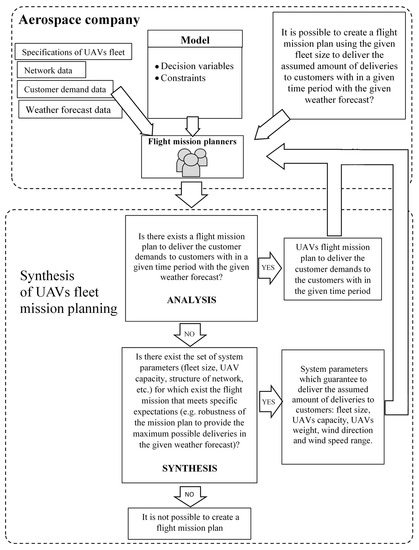
Figure 21.
Decision support of UAVs fleet mission planning.
When the answer is positive, the decision-maker can obtain the parameters of the system which guarantee to deliver the assumed amount of deliveries to the customers. A negative answer informs the decision-maker that it is impossible with the given inputs to find a flight mission plan. The conducted simulations of this study have been provided to aerospace companies, as a proposal input for a UAV fleet-planning decision support system enabling them to prototype alternative mission proposals for execution. Investigations on potential approaches and an offline-based system are carried out to ensure that only missions suitable to be sent to flight approval from air traffic control [47,48] are accepted and the results of the study will be implemented as a technical tool in the decision support systems of aerospace companies.
6. Conclusions
In this paper, a novel decision support-driven approach is presented to solve the complex problem of multi-trip fleet mission planning subject to changing weather conditions for a fleet UAVs. This problem involves the management of complex characteristics during the process of mission planning while considering factors such as weather dependencies, collision avoidance, and addressing the non-linear energy consumption behavior of UAVs that is affected by the weather conditions and the carrying payload.
In that context, the main problem can be seen a special case of the vehicle routing and scheduling problems, where the final flight plan consists of deliveries to customers that are arranged as a sequence of sub-missions. Therefore, the problem considered of UAVs mission planning match that of vehicle routing concerning the VRP which is NP-hard. Besides the presented UAVs fleet mission planning perspectives, the research scope regards a quite large class of logistics networks that share common properties even though they could have certain differences. In other words, besides UAVs that could be treated as a goods transport mode, other emerging trends concerning logistics and military issues can be modelled.
The proposed declarative decomposed solution approach offers a reasonable way to solve the problem reducing its complexity, and different alternative approaches could be tested in future research. The proposed approach leads to feasible solutions based on sufficient conditions that could be used as a prototype of a decision support system (DSS) addressing various influencing parameters involved in UAVs fleet-mission planning. Each sub-problem can be replaced by different alternatives in future research while ensuring the overall feasibility considering interdependency between the sub-problems to find optimal solutions. However, in further research, real-life verification of the method should be done by reducing the assumptions that have been made in this study, which constrain its application. Overall, this study should be used as a starting point for further research of online mission planning approaches, where the results of the study can be used to develop an interactive DSS that supports on-board UAV fleet-mission planning.
Author Contributions
Conceptualization was done by, A.T., G.B., B.Z. and P.N.; methodology, A.T. and G.B. validation, P.N., G.B. and B.Z.; formal analysis, A.T. and P.N.; data curation, A.T., G.B., and P.N.; writing-original draft preparation, A.T.; writing-review and editing, A.T., B.Z. and G.B.; supervision, G.B. and P.N.; project administration, A.T.; funding acquisition, P.N.
Funding
This research received no external funding.
Conflicts of Interest
The authors declare no conflict of interest.
References
- Bolton, G.E.; Katok, E. Learning-by-Doing in the Newsvendor Problem a Laboratory Investigation of the Role of Experience and Feedback. Manuf. Serv. Oper. Manag. 2004, 10, 519–538. [Google Scholar] [CrossRef]
- Avellar, G.S.C.; Pereira, G.A.S.; Pimenta, L.C.A.; Iscold, P. Multi-UAV routing for area coverage and remote sensing with minimum time. Sensors (Switzerland) 2015, 15, 27783–27803. [Google Scholar] [CrossRef] [PubMed]
- Khosiawan, Y.; Nielsen, I. A system of UAV application in indoor environment. Prod. Manuf. Res. 2016, 4, 2–22. [Google Scholar] [CrossRef]
- Barrientos, A.; Colorado, J.; Cerro, J.D.E.L.; Martinez, A.; Rossi, C.; Sanz, D.; Valente, J. Aerial Remote Sensing in Agriculture: A Practical Approach to Area Coverage and Path Planning for Fleets of Mini Aerial Robots. J. Field Robot. 2011, 667–689. [Google Scholar] [CrossRef]
- Bekhti, M.; Achir, N.; Boussetta, K.; Abdennebi, M. Drone Package Delivery: A Heuristic approach for UAVs path planning and tracking. EAI Endorsed Trans. Internet Things 2017, 3, e1. [Google Scholar] [CrossRef]
- Khosiawan, Y.; Scherer, S.; Nielsen, I. Toward delay-tolerant multiple-unmanned aerial vehicle scheduling system using Multi-strategy Coevolution algorithm. Adv. Mech. Eng. 2018, 10, 1687814018815235. [Google Scholar] [CrossRef]
- Kim, S.; Kim, Y. Optimum design of three-dimensional behavioural decentralized controller for UAV formation flight. Eng. Optim. 2009, 41, 199–224. [Google Scholar] [CrossRef]
- Thibbotuwawa, A.; Nielsen, P.; Zbigniew, B.; Bocewicz, G. Energy Consumption in Unmanned Aerial Vehicles: A Review of Energy Consumption Models and Their Relation to the UAV Routing. In International Conference on Information Systems Architecture and Technology; Springer: Berlin, Germany, 2019; pp. 173–184. [Google Scholar]
- Dorling, K.; Heinrichs, J.; Messier, G.G.; Magierowski, S. Vehicle Routing Problems for Drone Delivery. IEEE Trans Syst. Man Cybern. Syst. 2017, 47, 70–85. [Google Scholar] [CrossRef]
- AbdAllah, A.M.F.M.; Essam, D.L.; Sarker, R.A. On solving periodic re-optimization dynamic vehicle routing problems. Appl. Soft Comput. J. 2017, 55, 1–12. [Google Scholar] [CrossRef]
- Shetty, V.K.; Sudit, M.; Nagi, R. Priority-based assignment and routing of a fleet of unmanned combat aerial vehicles. Comput. Oper. Res. 2008, 35, 1813–1828. [Google Scholar] [CrossRef]
- Coelho, B.N.; Coelho, V.N.; Coelho, I.M.; Ochi, L.S.; Haghnazar, R.; Zuidema, D.; Lima, M.S.; da Costa, A.R. A multi-objective green UAV routing problem. Comput. Oper. Res. 2017, 88, 306–315. [Google Scholar] [CrossRef]
- Enright, J.J.; Frazzoli, E.; Pavone, M.; Ketan, S.A.V.L.A. Handbook of unmanned aerial vehicles. Handb. Unmanned Aer. Veh. 2015. [Google Scholar] [CrossRef]
- Guerriero, F.; Surace, R.; Loscrí, V.; Natalizio, E. A multi-objective approach for unmanned aerial vehicle routing problem with soft time windows constraints. Appl. Math. Model. 2014, 38, 839–852. [Google Scholar] [CrossRef]
- Sundar, K.; Venkatachalam, S.; Rathinam, S. An Exact Algorithm for a Fuel-Constrained Autonomous Vehicle Path Planning Problem. arXiv 2016. [Google Scholar] [CrossRef]
- Goerzen, C.; Kong, Z.; Mettler, B. A survey of motion planning algorithms from the perspective of autonomous UAV guidance. J. Intell. Robot. Syst. Theory Appl. 2010. [Google Scholar] [CrossRef]
- Khosiawan, Y.; Khalfay, A.; Nielsen, I. Scheduling unmanned aerial vehicle and automated guided vehicle operations in an indoor manufacturing environment using differential evolution-fused particle swarm optimization. Int. J. Adv. Robot. Syst. 2018, 15, 1729881417754145. [Google Scholar] [CrossRef]
- Wang, X.; Poikonen, S.; Golden, B. The Vehicle Routing Problem with Drones: A Worst-Case Analysis Outline Introduction to VRP Introduction to VRPD. Networks 2016, 1–22. [Google Scholar] [CrossRef]
- Bocewicz, G.; Nielsen, P.; Banaszak, Z.; Thibbotuwawa, A. A Declarative Modelling Framework for Routing of Multiple UAVs in a System with Mobile Battery Swapping Stations. In International Conference on Intelligent Systems in Production Engineering and Maintenance; Springer: Berlin, Germany, 2019; pp. 429–441. [Google Scholar]
- Ham, A.M. Integrated scheduling of m-truck, m-drone, and m-depot constrained by time-window, drop-pickup, and m-visit using constraint programming. Transp. Res. Part C Emerg. Technol. 2018, 91, 1–14. [Google Scholar] [CrossRef]
- Bocewicz, G.; Nielsen, P.; Banaszak, Z.; Thibbotuwawa, A. Routing and Scheduling of Unmanned Aerial Vehicles Subject to Cyclic Production Flow Constraints. In Proceedings of the 15th International Conference Distributed Computing and Artificial Intelligence, Toledo, Spain, 20–22 June 2018; pp. 75–86. [Google Scholar]
- Bocewicz, G.; Nielsen, P.; Banaszak, Z.; Thibbotuwawa, A. Deployment of Battery Swapping Stations for Unmanned Aerial Vehicles Subject to Cyclic Production Flow Constraints; Springer International Publishing: Berlin, Germany, 2018; pp. 73–87. [Google Scholar]
- Thibbotuwawa, A.; Nielsen, P.; Zbigniew, B.; Bocewicz, G. UAVs Fleet Mission Planning Subject to Weather Fore-Cast and Energy Consumption Constraints. Adv. Intell. Syst. Comput. 2019. [Google Scholar] [CrossRef]
- Thibbotuwawa, A.; Nielsen, P.; Zbigniew, B.; Bocewicz, G. Factors Affecting Energy Consumption of Unmanned Aerial Vehicles: An Analysis of How Energy Consumption Changes in Relation to UAV Routing. In International Conference on Information Systems Architecture and Technology; Springer: Berlin, Germany, 2019; pp. 228–238. [Google Scholar]
- Rathbun, D.; Kragelund, S.; Pongpunwattana, A.; Capozzi, B. An evolution based path planning algorithm for autonomous motion of a UAV through uncertain environments. In Proceedings of the 21st Digital Avionics Systems Conference 2010, Irvine, CA, USA, 27–31 October 2002; p. 8D2. [Google Scholar]
- Yang, G.; Kapila, V. Optimal path planning for unmanned air vehicles with kinematic and tactical constraints. In Proceedings of the Conference on Decision and Control, Las Vegas, NV, USA, 10–13 December 2002; Volume 2, pp. 1301–1306. [Google Scholar]
- Pohl, A.J.; Lamont, G.B. Multi-objective UAV mission planning using evolutionary computation. In Proceedings of the 2008 Winter Simulation Conference, Miami, FL, USA, 7–10 December 2008; pp. 1268–1279. [Google Scholar]
- Adbelhafiz, M.; Mostafa, A.; Girard, A. Vehicle Routing Problem Instances: Application to Multi-UAV Mission Planning. In Proceedings of the AIAA Guidance, Navigation, and Control Conference, Toronto, ON, Canada, 2–5 August 2010. [Google Scholar] [CrossRef]
- Belkadi, A.; Abaunza, H.; Ciarletta, L.; Castillo, P.; Theilliol, D. Distributed Path Planning for Controlling a Fleet of UAVs: Application to a Team of Quadrotors. IFAC-PapersOnLine 2017, 50, 15983–15989. [Google Scholar] [CrossRef]
- Kim, H.S.; Kim, Y. Trajectory optimization for unmanned aerial vehicle formation reconfiguration. Eng. Optim. 2014, 46, 84–106. [Google Scholar] [CrossRef]
- Song, B.D.; Park, K.; Kim, J. Persistent UAV delivery logistics: MILP formulation and efficient heuristic. Comput. Ind. Eng. 2018, 120, 418–428. [Google Scholar] [CrossRef]
- Maza, I.; Ollero, A. Multiple UAV cooperative searching operation using polygon area decomposition and efficient coverage algorithms. In Distributed Autonomous Robotic Systems 6; Alami, R., Chatila, R., Asama, H., Eds.; Springer: Japan, Tokyo, 2007; pp. 221–230. [Google Scholar]
- Habib, D.; Jamal, H.; Khan, S.A. Employing multiple unmanned aerial vehicles for co-operative path planning. Int. J. Adv. Robot Syst. 2013, 10, 235. [Google Scholar] [CrossRef]
- Liu, X.F.; Guan, Z.W.; Song, Y.Q.; Chen, D.S. An optimization model of UAV route planning for road segment surveillance. J. Cent. South Univ. 2014, 21, 2501–2510. [Google Scholar] [CrossRef]
- Xu, K.X.K.; Hong, X.H.X.; Gerla, M.G.M. Landmark routing in large wireless battlefield networks using UAVs. In Proceedings of the 2001 MILCOM Proceedings Communication Network-Centric Operations: Creating Information Force (Cat No01CH37277), McLean, VA, USA, 28–31 October 2001; Volume 1, pp. 230–234. [Google Scholar] [CrossRef]
- Mourelo Ferrandez, S.; Harbison, T.; Weber, T. Optimization of a truck-drone in tandem delivery network using k-means and genetic algorithm. J. Ind. Eng. Manag. 2016, 9, 374. [Google Scholar] [CrossRef]
- Sundar, K.; Rathinam, S. Algorithms for routing an unmanned aerial vehicle in the presence of refueling depots. IEEE Trans Autom. Sci. Eng. 2014, 11, 287–294. [Google Scholar] [CrossRef]
- Rubio, J.C.; Kragelund, S. The trans-pacific crossing: Long range adaptive path planning for UAVs through variable wind fields. In Proceedings of the Digital Avionics System Conference 2003. DASC’03. 22nd, Indianapolis, IN, USA, 12–16 October 2003; p. 8-B. [Google Scholar]
- Nguyen, T.; Tsz-Chiu, A. Extending the Range of Delivery Drones by Exploratory Learning of Energy Models. In Proceedings of the 16th Conference on Autonomous Agents and MultiAgent Systems, São Paulo, Brazil, 8–12 May 2017; pp. 1658–1660. [Google Scholar]
- Chaieb, M.; Jemai, J.; Mellouli, K. On the Relationships Between Sub Problems in the Hierarchical Optimization Framework. In International Conference on Industrial, Engineering and Other Applications of Applied Intelligent Systems; Ali, M., Kwon, Y.S., Lee, C.H., Kim, Y., Eds.; Springer International Publishing, Cham: Berlin, Germany, 2015; pp. 232–241. [Google Scholar]
- Liu, X.; Gao, L.; Guang, Z.; Song, Y. A UAV Allocation Method for Traffic Surveillance in Sparse Road Network. J. Highw. Transp. Res. Dev. 2013, 7, 81–87. [Google Scholar] [CrossRef]
- Korf, R.E. Depth-first iterative-deepening. Artif. Intell. 2003, 27, 97–109. [Google Scholar] [CrossRef]
- Barták, R. Incomplete Depth-First Search Techniques: A Short Survey. In Proceedings of the 6th Workshop on Constraint Programming for Decision and Control, Gliwice, Poland, 29 June 2004; pp. 1–8. [Google Scholar]
- Fügenschuh, A.; Müllenstedt, D. Flight Planning for Unmanned Aerial Vehicles. Professur für Angewandte Mathematik, Helmut-Schmidt-Universität. In Angewandte Mathematik und Optimierung Schriftenreihe/Applied Mathematics and Optimization Series; Universität der Bundeswehr Hamburg: Hamburg, Germany, 2015. [Google Scholar]
- Available online: https://www.gurobi.com/pdfs/Gurobi-Corporate-Brochure.pdf (accessed on 2 July 2019).
- Radzki, G.; Thibbotuwawa, A.; Bocewicz, G. UAVs flight routes optimization in changing weather conditions—Constraint programming approach. Appl. Comput. Sci. 2019, 15, 5–17. [Google Scholar] [CrossRef]
- Danish Transport Authority Future Regulation of Civil Drones. Report from an Inter-Ministerial Working 2015 Group. Available online: https://www.trafikstyrelsen.dk (accessed on 7 May 2019).
- Allouche, M. The integration of UAVs in airspace. Air. Sp. Eur. 2000, 2, 101–104. [Google Scholar] [CrossRef]
© 2019 by the authors. Licensee MDPI, Basel, Switzerland. This article is an open access article distributed under the terms and conditions of the Creative Commons Attribution (CC BY) license (http://creativecommons.org/licenses/by/4.0/).