FSRFNet: Feature-selective and Spatial Receptive Fields Networks

Featured Application

This work can be used in many fields, such as robot navigation, intelligent video monitoring, industrial detection, etc.

Abstract

The attention mechanism plays a crucial role in the human visual experience. In the cognitive neuroscience community, the receptive field size of visual cortical neurons is regulated by the additive effect of feature-selective and spatial attention. We propose a novel architectural unit called a “Feature-selective and Spatial Receptive Fields” (FSRF) block that implements adaptive receptive field sizes of neurons through the additive effects of feature-selective and spatial attention. We show that FSRF blocks can be inserted into the architecture of existing convolutional neural networks to form an FSRF network architecture, and test its generalization capabilities on different datasets.

1. Introduction

In recent years, the field of computer vision has undergone tremendous changes, with deep learning becoming a powerful tool. Owing to its data-driven nature and the availability of massively parallel computing, deep neural networks have achieved state-of-the-art results in most areas, and researchers have designed many advanced network architectures [1,2,3,4,5,6,7,8,9,10,11,12]. The ImageNet competition champion AlexNet [8] was the first to apply convolutional neural networks (CNNs) to a deep network. Subsequently, more deep neural network architectures have been proposed, such as VGGNet [1], GoogLeNet [2], ResNet [6], WideResNet [7], ResNeXt [9], Xception [10], MobileNet [11], and DenseNet [12]. Many other visual recognition algorithms [13,14,15,16,17,18,19,20,21,22] have been inspired by these designs, notably [1,2,6,8]. With improvements in detection accuracy and real-time performance, the object detection algorithm based on deep learning has gradually developed into two types: the two-stage approach and one-stage approach. The one-stage approach [19,20,21,22] incorporates training and detection in a network and solves object detection as a regression problem. Compared with the two-stage approach [13,16,17,18], the one-stage approach has a better real-time performance while maintaining better detection accuracy.

In addition to deep learning and object detection methods, previous research has studied the importance of attention [23,24,25]. We focus on the interaction between feature-selective and spatial attention and the impact on receptive fields (RFs). The classical RF (CRF) of neurons in the V1 region was discussed in [26]. Researchers have proposed that in such a visual zone as the V4 region, attention should be paid to the effects of neuronal discharge rates in two ways [27]. One is the input gating model. In this model, the RF of the mediators in the theory corresponds to the stimulus that is noted or ignored in the field of view. Another theory is the neuronal strobing model, which states that neurons in the V4 region themselves have enhanced and inhibited effects on attention. In addition, Nelson et al. [28] found that stimulation outside the CRF also affected neuronal responses. [29,30,31,32] report important interactions between feature-selective and spatial attention, and each type of attention enhances the effect of another type of attention. Moreover, SKNet [33] propose Selective Kernel Networks with a Selective Kernel convolution, to aggregate information from multiple kernels to realize the adaptive RF sizes of neurons in a nonlinear approach. However, SKNet [33] may be insufficient to provide neurons with powerful adaptation ability.

In this paper, we propose a novel architectural unit called a “Feature-selective and Spatial Receptive Fields” (FSRF) block that implements adaptive RF sizes of neurons through the additive effects of feature-selective and spatial attention. To achieve this, we use a set of operators in the FSRF block: Multi-branch Convolution, Fuse, and Interactions between Feature-selective and Spatial Attention. The Multi-branch Convolution generates multiple paths corresponding to different RF sizes. The Fuse operator combines information from multiple paths to obtain a global weight representation. The Interactions between Feature-selective and Spatial Attention operator aggregates feature maps of different RF sizes according to the additive effects of feature-selective and spatial attention. The structure of the FSRF block is simple and can be used directly in the state-of-the-art architectures currently available. Besides, the problem of fast objects recognition is also very important in monitoring the electromagnetic environment where signals generated by different types of emitters (radars, jammers) are in many situations noisy, misshaped or changing in relation to the weather condition, task and application, thus the FSRF network (FSRFNet) may also be directly applied in recognition and identification emitter signals [34,35,36,37].

Main contributions of this work are summarized as follows: (1) We propose a simple and effective attention block (FSRF) that can be widely applied to boost representation power of CNNs; (2) We validate the effectiveness of the FSRF block through extensive ablation studies; (3) We demonstrate that the FSRFNet outperforms previous state-of-the-art models on datasets of different sizes, and successfully embed an FSRF block into lightweight models (e.g., ShuffleNetV2 [38] and MobileNetV2 [39]).

2. Related Work

2.1. Deeper Architectures

Convolutional neural networks (CNNs) exhibit excellent performance when dealing with visual tasks owing to their rich characterization capabilities [8,40]. In visual research, well-designed network architectures can significantly improve performance in a variety of applications. Increasing the depth of the neural network is a simple and effective design method in neural network design. VGGNet [1] and GoogLeNet [2] show that increasing the depth of the network can significantly improve the ability of model learning representation. However, as the network becomes increasingly deeper, gradient propagation becomes more difficult. Batch normalization [3] improves the stability of the network while learning by adjusting the distribution of each layer of input in the network. By using a well-designed multi-branch architecture, inception models [2,3,4,5] enable a more flexible convolutional combination and improve the network’s feature learning capabilities. Further improvements have been achieved. Firstly, in order to alleviate the problem of gradient disappearance caused by increasing network depth, ResNet [6] proposes an identity-based skip connection, which makes it possible to achieve a better learning ability in deeper networks. WideResNet [7] shows that using more channels and a wider convolution in the network model can improve performance. ResNeXt [9] and Xception [10] prove that grouped convolutions can improve the accuracy of classification. MobileNet [11] uses depthwise separable convolutions to enable the network to be applied on mobile terminals. Finally, DenseNet [12] is a densely connected network architecture proposed by Huang et al., which provides maximum information transmission between layers in the network.

2.2. Attention Mechanisms

Evidence from the human perception process [23] illustrates the importance of the attention mechanism. Attention is generally divided into two types: top-down conscious attention and bottom-up unconscious attention. It is worth noting that the mechanism uses top-down information to guide the bottom-up feed-forward process, which biases the distribution of the most informative feature expressions while suppressing the less useful [41,42,43]. Attention is the ability to focus perception on a stimulus while ignoring other potential stimuli. It has proven to be one of the most interesting areas of research in cognitive neuroscience. The benefits of the attention mechanism have been demonstrated in many tasks, including neuro-machine translation [44], image subtitles [45], and lip reading [46]. In order to enhance the performance of image classification, some researchers have introduced attention mechanisms into their network models [33,47,48]. In Brad Motter’s neurophysiological study of attention in macaque monkeys [49], all regions of the visual cortex showed a greater sensitivity to attention when the target stimulus was presented with competing stimuli, compared to the condition when the target stimulus was presented alone. Another study of macaques similarly found that attention regulated sensory responses in areas V2 and V4 primarily when two or more simultaneous stimuli competed for access to a neuron’s receptive field; no such effect was observed when only a single stimulus was inside the receptive field [50]. An fMRI study found that selective attention in humans modulates neural activity in the visual cortex through top-down biasing signals [48]. When a monkey or a person is asked to pay attention to a particular area of space, corresponding increases in neural activity can be observed in V1, V2, and V4 [49,50,51]. Such activation enhancement is described as a “gain” of the sensory process [52] or as an increase in neuronal sensitivity. [29,30,31,32] show that there is a small but significant interaction between feature-selective and spatial attention. Recent research [53] suggests that feature-based attention operates in a spatially global manner throughout the field of view, and that the spatial focus of attention should be carefully controlled to maximize the global feature-based attention effect.

3. Feature-selective and Spatial Receptive Fields (FSRF) Blocks

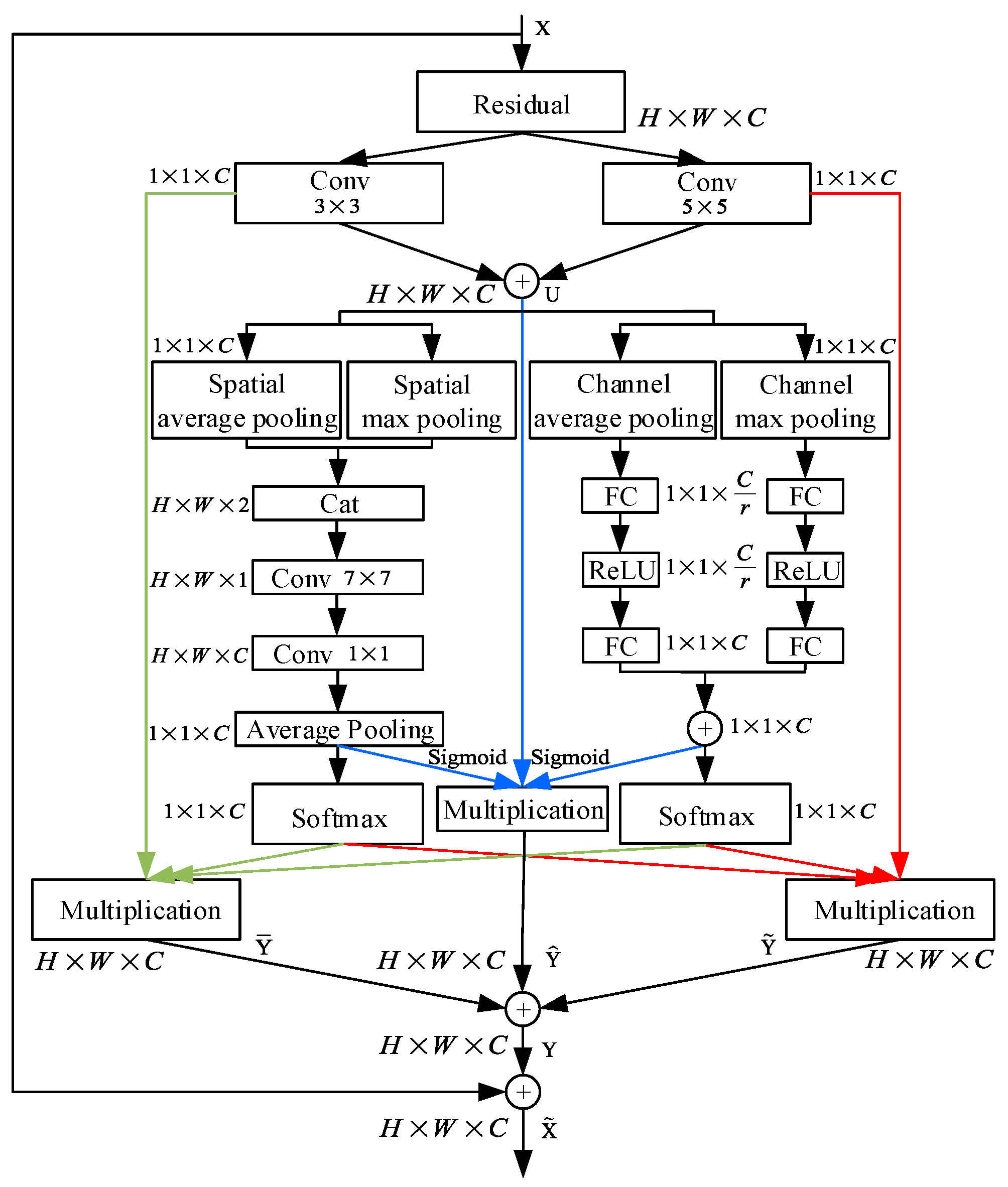
In order to implement adaptive receptive field (RF) sizes of neurons through the additive effects of feature-selective and spatial attention, we propose a novel architectural unit called a “Feature-selective and Spatial Receptive Fields” (FSRF) block. The structure of the FSRF block is depicted in Figure 1. We implement the FSRF block via three operations: Multi-branch Convolution, Fuse, and Interactions between Feature-selective and Spatial Attention.

3.1. Multi-Branch Convolution

The goal of using multi-branch convolution is to provide various filters for multiple branches, ultimately aggregating more informative and multifarious features. For any given feature map $\mathrm{X}\in {ℝ}^{H^{\prime }\times W^{\prime }\times C^{\prime }}$, firstly we conduct two transformations ${\overline{\mathrm{F}}}_{\mathrm{tr}}$: $\mathrm{X}\to \overline{\mathrm{U}}\in {ℝ}^{H\times W\times C}$ and ${\tilde{\mathrm{F}}}_{\mathrm{tr}}$: $\mathrm{X}\to \tilde{\mathrm{U}}\in {ℝ}^{H\times W\times C}$. Note that ${\overline{\mathrm{F}}}_{\mathrm{tr}}$ and ${\tilde{\mathrm{F}}}_{\mathrm{tr}}$ are composed of efficient convolutions, with batch normalization and ReLU functioning in sequence. A $3\times 3$ convolution kernel is used in the transformation ${\overline{\mathrm{F}}}_{\mathrm{tr}}$, and a $5\times 5$ convolution kernel is used in the transformation ${\tilde{\mathrm{F}}}_{\mathrm{tr}}$. H, W, and C denote the height, width, and number of channels of the feature map, respectively. Let ${\mathrm{W}}_c=\left[{\mathrm{w}}_1,{\mathrm{w}}_2,\dots ,{\mathrm{w}}_c\right]$ and ${\mathrm{O}}_c=\left[{\mathrm{o}}_1,{\mathrm{o}}_2,\dots ,{\mathrm{o}}_c\right]$ denote the learned set of $3\times 3$ and $5\times 5$ convolution kernels, where ${\mathrm{W}}_c$ and ${\mathrm{O}}_c$ refers to the parameters of the corresponding c-th convolution kernel. We can then write the outputs of ${\overline{\mathrm{F}}}_{\mathrm{tr}}$ and ${\tilde{\mathrm{F}}}_{\mathrm{tr}}$ as ${\overline{\mathrm{U}}}_c=\left[{\overline{\mathrm{u}}}_1,{\overline{\mathrm{u}}}_2,\dots ,{\overline{\mathrm{u}}}_c\right]$ and ${\tilde{\mathrm{U}}}_c=\left[{\tilde{\mathrm{u}}}_1,{\tilde{\mathrm{u}}}_2,\dots ,{\tilde{\mathrm{u}}}_c\right]$, where

$${\overline{\mathrm{u}}}_c={\mathrm{w}}_c\ast \mathrm{X}={\displaystyle \sum _{\mathrm{s}=1}^{{\mathrm{C}}^{\prime }}{\mathrm{w}}_c^{\mathrm{s}}\ast {\mathrm{x}}^{\mathrm{s}}},{\tilde{\mathrm{u}}}_c={\mathrm{o}}_c\ast \mathrm{X}={\displaystyle \sum _{\mathrm{s}=1}^{{\mathrm{C}}^{\prime }}{\mathrm{o}}_c^{\mathrm{s}}\ast {\mathrm{x}}^{\mathrm{s}}}$$

(1)

Here $\ast$ denotes convolution, ${\mathrm{w}}_c=\left[{\mathrm{w}}_1^{\mathrm{s}},{\mathrm{w}}_2^{\mathrm{s}},\dots ,{\mathrm{w}}_c^{\mathrm{s}}\right]$, ${\mathrm{o}}_c=\left[{\mathrm{o}}_1^{\mathrm{s}},{\mathrm{o}}_2^{\mathrm{s}},\dots ,{\mathrm{o}}_c^{\mathrm{s}}\right]$ and $\mathrm{X}=\left[{\mathrm{x}}^1,{\mathrm{x}}^2,\dots ,{\mathrm{x}}^{{\mathrm{C}}^{\prime }}\right]$. ${\mathrm{w}}_c^{\mathrm{s}}$ and ${\mathrm{o}}_c^{\mathrm{s}}$ is a 2D spatial kernel representing a single channel of ${\mathrm{w}}_c$ and ${\mathrm{o}}_c$, respectively.

3.2. Fuse

Our goal is to enable neurons to adaptively adjust their RF sizes through the additive effects of feature-selective and spatial attention. The basic idea is to use two gates from the average and max channel (AMC) and average and max spatial (AMS) attention building blocks to control the flow of multiple branches carrying different scales of information into neurons in the next layer. We first combine the results of multiple branches (such as the two shown in Figure 1) by summing the elements, as follows:

$$\mathrm{U}=\overline{\mathrm{U}}+\tilde{\mathrm{U}}$$

(2)

We then input the feature map obtained from the previous step into the AMC and AMS attention building blocks, and flexibly select different information-space scales under the guidance of compact feature descriptors.

The structure of the AMC attention building block is depicted in Figure 2. The AMC attention building block generates a channel attention map by using the inter-channel relationship of features. To compute the channel attention efficiently, we squeeze the spatial dimension of the input feature map into a channel descriptor by using global average pooling and global max pooling. We describe the detailed operation below.

The preprocessed feature map U passes through two branches of the AMC attention building block. The first branch uses global average pooling to generate channel-wise statistics. Finally, a statistic $\overline{\mathrm{z}}\in {ℝ}^C$ is generated by shrinking U through its spatial dimensions $H\times W$, such that the c-th element of $\overline{\mathrm{z}}$ is calculated by:

$${\overline{z}}_c={\mathrm{F}}_{ga}\left({\mathrm{u}}_c\right)=\frac{1}{H\times W}{\displaystyle \sum _{i=1}^H{\displaystyle \sum _{j=1}^W{u}_c\left(i,j\right)}}$$

(3)

where ${\mathrm{F}}_{ga}\left({\mathrm{u}}_c\right)$ indicates the global average pooling operator.

Further, in order to take advantage of the information aggregated in the global average pooling, we then conduct a second operation, the purpose of which is to make full use of the dependencies between different feature maps. In order to achieve this effect, we use a dimensionality-reduction layer with parameters ${\mathrm{T}}_1$ and reduction ratio r, a ReLU layer, and a dimensionality-increasing layer with parameters ${\mathrm{T}}_2$. The fully connected layers are used in the dimensionality-reduction layer and dimensionality-increasing layer. The average attention of the channel is computed as:

$$\overline{\mathrm{s}}={\mathrm{F}}_{ex}\left({\overline{\mathrm{z}}}_c,\mathrm{T}\right)={\mathrm{T}}_2\delta \left({\mathrm{T}}_1\overline{\mathrm{z}}\right)$$

(4)

where $\delta$ refers to the ReLU function, ${\mathrm{T}}_1\in {ℝ}^{\frac{C}{r}\times C}$, and ${\mathrm{T}}_2\in {ℝ}^{C\times \frac{C}{r}}$.

The second branch uses global max pooling to generate channel-wise statistics. A statistic $\tilde{\mathrm{z}}\in {ℝ}^C$ is generated by shrinking U through its spatial dimensions $H\times W$, such that the c-th element of $\tilde{\mathrm{z}}$ is calculated by:

$${\tilde{z}}_c={\mathrm{F}}_{gm}\left({\mathrm{u}}_c\right)=\max \left({\displaystyle \sum _{i=1}^H{\displaystyle \sum _{j=1}^W{u}_c\left(i,j\right)}}\right)$$

(5)

where ${\mathrm{F}}_{gm}\left({\mathrm{u}}_c\right)$ indicates the global average pooling operator.

Additionally, we conduct a second operation in order to take advantage of the information aggregated in the global max pooling, the purpose of which, as with the first branch, is to make full use of the dependencies between different feature maps. The maximum attention of the channel is computed as:

$$\tilde{\mathrm{s}}={\mathrm{F}}_{ex}\left(\tilde{\mathrm{z}},\mathrm{T}\right)={\mathrm{T}}_2\delta \left({\mathrm{T}}_1\tilde{\mathrm{z}}\right)$$

(6)

Finally, a multiplication activation function is used to process the feature information of the two branch outputs:

$$\mathrm{s}={\mathrm{F}}_{add}\left(\overline{\mathrm{s}},\tilde{\mathrm{s}}\right)=\overline{\mathrm{s}}+\tilde{\mathrm{s}}$$

(7)

where $\mathrm{s}\in {ℝ}^C$. The ${\mathrm{F}}_{add}\left(\overline{\mathrm{s}},\tilde{\mathrm{s}}\right)$ indicates the channel-wise summation between $\overline{\mathrm{s}}$ and $\tilde{\mathrm{s}}$.

The structure of the AMS attention building block is depicted in Figure 3. The role of the AMS attention building block is to produce a spatial attention map by exploiting the inter-spatial relationship of features. we first apply global average pooling and global max pooling operations along the channel axis to generate an efficient feature descriptor, respectively, and then concatenate the previous two feature maps together. Based on the concatenated feature descriptors, we use a convolution layer to generate a spatial attention map. In order to use the spatial attention map by gated operation, we apply a convolution layer with c channels and a global average pooling operation after the last convolution layer. We describe the detailed operation below.

For a preprocessed feature map U, firstly we conduct two transformations ${\mathrm{H}}_{mean}$: $\mathrm{U}\to \overline{\mathrm{V}}\in {ℝ}^{H\times W\times 1}$ and ${\mathrm{H}}_{max}$: $\mathrm{U}\to \tilde{\mathrm{V}}\in {ℝ}^{H\times W\times 1}$. These are connected together to create the spatial attention map ${\mathrm{M}}^{\prime }\in {ℝ}^{H\times W\times 2}$:

$${\mathrm{M}}^{\prime }=\mathrm{c}\mathrm{a}\mathrm{t}\left(\overline{\mathrm{V}},\tilde{\mathrm{V}}\right)=\mathrm{c}\mathrm{a}\mathrm{t}\left({\mathrm{H}}_{mean}\left(\mathrm{U}\right),{\mathrm{H}}_{max}\left(\mathrm{U}\right)\right)$$

(8)

The map is then convoluted by a 7 × 7 filter to produce a 2D spatial attention map ${\mathrm{M}}^{″}\in {ℝ}^{H\times W}$:

$${\mathrm{M}}^{″}={\mathrm{F}}^{7\times 7}\left(\mathrm{c}\mathrm{a}\mathrm{t}\left({\mathrm{H}}_{mean}\left(\mathrm{U}\right),{\mathrm{H}}_{max}\left(\mathrm{U}\right)\right)\right)$$

(9)

The 2D spatial attention map generated in the previous step, then resulting in a multidimensional spatial attention map $\mathrm{M}\in {ℝ}^{H\times W\times C}$:

$$\mathrm{M}={\mathrm{F}}^{1\times 1}\left({\mathrm{F}}^{7\times 7}\left(\mathrm{c}\mathrm{a}\mathrm{t}\left({\mathrm{H}}_{mean}\left(\mathrm{U}\right),{\mathrm{H}}_{max}\left(\mathrm{U}\right)\right)\right)\right)$$

(10)

where ${\mathrm{F}}^{1\times 1}$ represents a convolution operation with the filter size of $1\times 1$, ${\mathrm{F}}^{7\times 7}$ represents a convolution operation with the filter size of $7\times 7$, and ‘cat’ denotes the concatenate function. ${\mathrm{H}}_{mean}\left(\mathrm{U}\right)$ and ${\mathrm{H}}_{max}\left(\mathrm{U}\right)$ refer to global average pooling and global max pooling operations along the corresponding channel axis.

We then use global average pooling to generate channel-wise statistics. A statistic $\mathrm{n}\in {ℝ}^C$ is generated by shrinking M through its spatial dimensions $H\times W$, such that the c-th element of n is calculated by:

$$n_c={\mathrm{F}}_{ga}\left({\mathrm{m}}_c\right)=\frac{1}{H\times W}{\displaystyle \sum _{i=1}^H{\displaystyle \sum _{j=1}^W{m}_c\left(i,j\right)}}$$

(11)

3.3. Interactions between Feature-selective and Spatial Attention

In order to take advantage of the information aggregated in the AMC and AMS attention building blocks, we conduct a soft attention across channels that achieves interactions between feature-selective and spatial attention. Firstly, a SoftMax operator is applied on the channel-wise digits at the output of the AMC building block:

$$a_c=\frac{e^{{\mathrm{A}}_c\mathrm{s}}}{e^{{\mathrm{A}}_c\mathrm{s}}+e^{{\mathrm{B}}_c\mathrm{s}}},b_c=\frac{e^{{\mathrm{B}}_c\mathrm{s}}}{e^{{\mathrm{A}}_c\mathrm{s}}+e^{{\mathrm{B}}_c\mathrm{s}}}$$

(12)

Similarly, a SoftMax operator is applied on the channel-wise digits at the output of the AMS building block:

$$c_c=\frac{e^{{\mathrm{J}}_c\mathrm{n}}}{e^{{\mathrm{J}}_c\mathrm{n}}+e^{{\mathrm{K}}_c\mathrm{n}}},d_c=\frac{e^{{\mathrm{K}}_c\mathrm{n}}}{e^{{\mathrm{J}}_c\mathrm{n}}+e^{{\mathrm{K}}_c\mathrm{n}}}$$

(13)

where $\mathrm{A},\mathrm{B},\mathrm{J},\mathrm{K}\in {ℝ}^{C\times \frac{C}{r}}$, a and c denote the vector for $\overline{\mathrm{U}}$, and b and d denote the vector for $\tilde{\mathrm{U}}$. Note that $a_c$ is the c-th element of a and ${\mathrm{A}}_c\in {ℝ}^{1\times \frac{C}{r}}$ is the c-th row of A; likewise for $b_c$, ${\mathrm{B}}_c$, $c_c$, ${\mathrm{J}}_c$, $d_c$ and ${\mathrm{K}}_c$.

A simple sigmoid operator is applied on the channel-wise digits at the output of the AMC building block:

$$e_c=\sigma \left({\mathrm{s}}_c\right)$$

(14)

Similarly, a simple sigmoid operator is applied on the channel-wise digits at the output of the AMS building block:

$$f_c=\sigma \left({\mathrm{n}}_c\right)$$

(15)

The feature maps $\overline{\mathrm{Y}}$, $\widehat{\mathrm{Y}}$ and $\tilde{\mathrm{Y}}$ are obtained by rescaling the transformation output $\overline{\mathrm{U}}$, $\mathrm{U}$ and $\tilde{\mathrm{U}}$ with the activations:

$$\begin{array}{l}{\overline{\mathrm{Y}}}_c={\mathrm{F}}_{mul}\left({\overline{\mathrm{u}}}_c,a_c,c_c\right)={\overline{\mathrm{u}}}_c\cdot a_c\cdot c_c\\ {\widehat{\mathrm{Y}}}_c={\mathrm{F}}_{mul}\left({\mathrm{u}}_c,e_c,f_c\right)={\mathrm{u}}_c\cdot e_c\cdot f_c\\ {\tilde{\mathrm{Y}}}_c={\mathrm{F}}_{mul}\left({\tilde{\mathrm{u}}}_c,b_c,d_c\right)={\tilde{\mathrm{u}}}_c\cdot b_c\cdot d_c\end{array}$$

(16)

where $\overline{\mathrm{Y}}=\left[{\overline{\mathrm{Y}}}_1,{\overline{\mathrm{Y}}}_2,\dots ,{\overline{\mathrm{Y}}}_c\right],{\overline{\mathrm{Y}}}_c\in {ℝ}^{H\times W}$ and likewise for $\widehat{\mathrm{Y}}$ and $\tilde{\mathrm{Y}}$. ${\mathrm{F}}_{mul}\left({\overline{\mathrm{u}}}_c,a_c,c_c\right)$ refers to channel-wise multiplication between the scalar $a_c$, $c_c$ and the feature map ${\overline{\mathrm{u}}}_c$, and likewise for ${\mathrm{F}}_{mul}\left({\mathrm{u}}_c,e_c,f_c\right)$ and ${\mathrm{F}}_{mul}\left({\tilde{\mathrm{u}}}_c,b_c,d_c\right)$. The final feature map $\mathrm{Y}$ is obtained by the element-wise summation of the vectors $\overline{\mathrm{Y}}$, $\widehat{\mathrm{Y}}$ and $\tilde{\mathrm{Y}}$:

$${\mathrm{Y}}_c=\overline{\mathrm{Y}}+\widehat{\mathrm{Y}}+\tilde{\mathrm{Y}}={\overline{\mathrm{u}}}_c\cdot a_c\cdot c_c+{\mathrm{u}}_c\cdot e_c\cdot f_c+{\tilde{\mathrm{u}}}_c\cdot b_c\cdot d_c,a_c+b_c=1,c_c+d_c=1$$

(17)

where $\mathrm{Y}=\left[{\mathrm{Y}}_1,{\mathrm{Y}}_2,\dots ,{\mathrm{Y}}_c\right],{\mathrm{Y}}_c\in {ℝ}^{H\times W}$.

3.4. Instantiation

The FSRF block can be integrated into a standard architecture such as ResNet [6] with a non-linear insertion after each convolution. In addition, the flexibility of the FSRF block means that it can be applied directly to conversions beyond standard convolution.

Here, FSRF blocks are used with residual modules. By making this change to each such module in the architecture, we can obtain an FSRF-ResNet network. Figure 4 depicts the schema of an FSRF-ResNet module. Further variants that integrate FSRF blocks with ResNeXt [9], ShuffleNetV2 [38], and MobileNetV2 [39] can be constructed by following similar schemes, as discussed below.

4. Network Architecture

An FSRF network (FSRFNet) can be constructed by simply stacking a set of FSRF blocks. For concrete examples of FSRFNet architectures, a detailed description of FSRF-50 is presented in

Table 1. Network architecture based on the ResNeXt-50 backbone.

Output	ResNeXt-50 (32× 4d)	SENet-50	SKNet-50	FSRFNet-50
$112\times 112$		$\mathrm{conv},7\times 7,64,\mathrm{stride}2$
$112\times 112$		$\max \mathrm{pool},3\times 3,\mathrm{stride}2$
$56\times 56$	$\left[\begin{array}{l}1\times 1,128\\ 3\times 3,128,G=32\\ 1\times 1,256\end{array}\right]\times 3$	$\left[\begin{array}{l}1\times 1,128\\ 3\times 3,128,G=32\\ 1\times 1,256\\ fc,\left[16,256\right]\end{array}\right]\times 3$	$\left[\begin{array}{l}1\times 1,128\\ \mathrm{SK}\left[\begin{array}{l}M=2,G=32,\\ r=16\end{array}\right],128\\ 1\times 1,256\end{array}\right]\times 3$	$\left[\begin{array}{l}1\times 1,128\\ \mathrm{FSRF}\left[\begin{array}{l}M=2,G=32,\\ r=16\end{array}\right],128\\ 1\times 1,512\end{array}\right]\times 3$
$28\times 28$	$\left[\begin{array}{l}1\times 1,256\\ 3\times 3,256,G=32\\ 1\times 1,512\end{array}\right]\times 4$	$\left[\begin{array}{l}1\times 1,256\\ 3\times 3,256,G=32\\ 1\times 1,512\\ fc,\left[32,512\right]\end{array}\right]\times 4$	$\left[\begin{array}{l}1\times 1,256\\ \mathrm{SK}\left[\begin{array}{l}M=2,G=32,\\ r=16\end{array}\right],256\\ 1\times 1,512\end{array}\right]\times 4$	$\left[\begin{array}{l}1\times 1,256\\ \mathrm{FSRF}\left[\begin{array}{l}M=2,G=32,\\ r=16\end{array}\right],256\\ 1\times 1,512\end{array}\right]\times 4$
$14\times 14$	$\left[\begin{array}{l}1\times 1,512\\ 3\times 3,512,G=32\\ 1\times 1,1024\end{array}\right]\times 6$	$\left[\begin{array}{l}1\times 1,512\\ 3\times 3,512,G=32\\ 1\times 1,1024\\ fc,\left[64,1024\right]\end{array}\right]\times 6$	$\left[\begin{array}{l}1\times 1,512\\ \mathrm{SK}\left[\begin{array}{l}M=2,G=32,\\ r=16\end{array}\right],512\\ 1\times 1,1024\end{array}\right]\times 6$	$\left[\begin{array}{l}1\times 1,512\\ \mathrm{FSRF}\left[\begin{array}{l}M=2,G=32,\\ r=16\end{array}\right],512\\ 1\times 1,1028\end{array}\right]\times 6$
$7\times 7$	$\left[\begin{array}{l}1\times 1,1024\\ 3\times 3,1024,G=32\\ 1\times 1,2048\end{array}\right]\times 3$	$\left[\begin{array}{l}1\times 1,1024\\ 3\times 3,1024,G=32\\ 1\times 1,2048\\ fc,\left[128,2048\right]\end{array}\right]\times 3$	$\left[\begin{array}{l}1\times 1,1024\\ \mathrm{SK}\left[\begin{array}{l}M=2,G=32,\\ r=16\end{array}\right],1024\\ 1\times 1,2048\end{array}\right]\times 3$	$\left[\begin{array}{l}1\times 1,1024\\ \mathrm{FSRF}\left[\begin{array}{l}M=2,G=32,\\ r=16\end{array}\right],1024\\ 1\times 1,2048\end{array}\right]\times 3$
$1\times 1$		$\mathrm{global}\mathrm{average},1000-d\mathrm{fc},\mathrm{soft}\max$

* The four columns show the architectures of ResNeXt-50 with a 32×4d template, SENet-50, SKNet-50, and FSRFNet-50. Filter sizes and feature dimensionalities of a residual block are shown inside the brackets; the number of stacked blocks for each stage is shown outside the brackets.

. It is recommended that FSRFNet consists primarily of a bunch of duplicate bottlenecks called “FSRF units,” in a similar fashion to ResNeXt [9]. Each FSRF unit consists of a series of $1\times 1$ convolutions, FSRF blocks, and further $1\times 1$ convolutions. In ResNeXt [9], large kernel convolutions in all original bottleneck blocks are replaced by the proposed FSRF blocks. FSRF-50 uses {3, 4, 6, 3} FSRF units. Table 1 shows a 50-layer FSRFNet-50 architecture with four phases, using {3, 4, 6, 3} FSRF units. Different architectures can be obtained by changing the number of FSRF units per stage.

In the FSRF units of the FSRF-50, the reduction ratio of the number of parameters in the control fuse operator determines the final setting of the FSRF block. There are two important hyperparameters that determine this final setting: the group number G that controls the cardinality of each path and the reduction ratio r of the number of parameters in the control fuse operator. In Table 1, we set the reduction ratio r = 16 and cardinality G = 32.

5. Experiments

In this section, we conduct experiments to study the effectiveness of the FSRF block in a range of tasks, datasets, and model architectures. To benchmark, we compare single crop top-1 performance on datasets of different sizes.

5.1. Tiny ImageNet Classification

Tiny ImageNet [54] has 200 classes. Each class has 500 training images, 50 validation images, and 50 test images. We train the network on the training set and report the top-1 errors on the validation set. For data enhancement, we follow standard practices and perform random size cropping to 224 × 224 and random horizontal flipping [2]. We use synchronous SGD with a momentum of 0.9, a mini-batch size of 32, and a weight decay of 1 × 10⁻⁴. The initial learning rate is set to 0.5 and decreased by a factor of 10 every 30 epochs. All models are trained for 100 epochs from scratch on one GPU, using the weight initialization strategy in [55]. We first compare FSRFNet-50 and FSRFNet-101 with a publicly competitive model of similar complexity. The results show that the FSRF block is consistent in improving the performance of state-of-the-art attention-based CNNs.

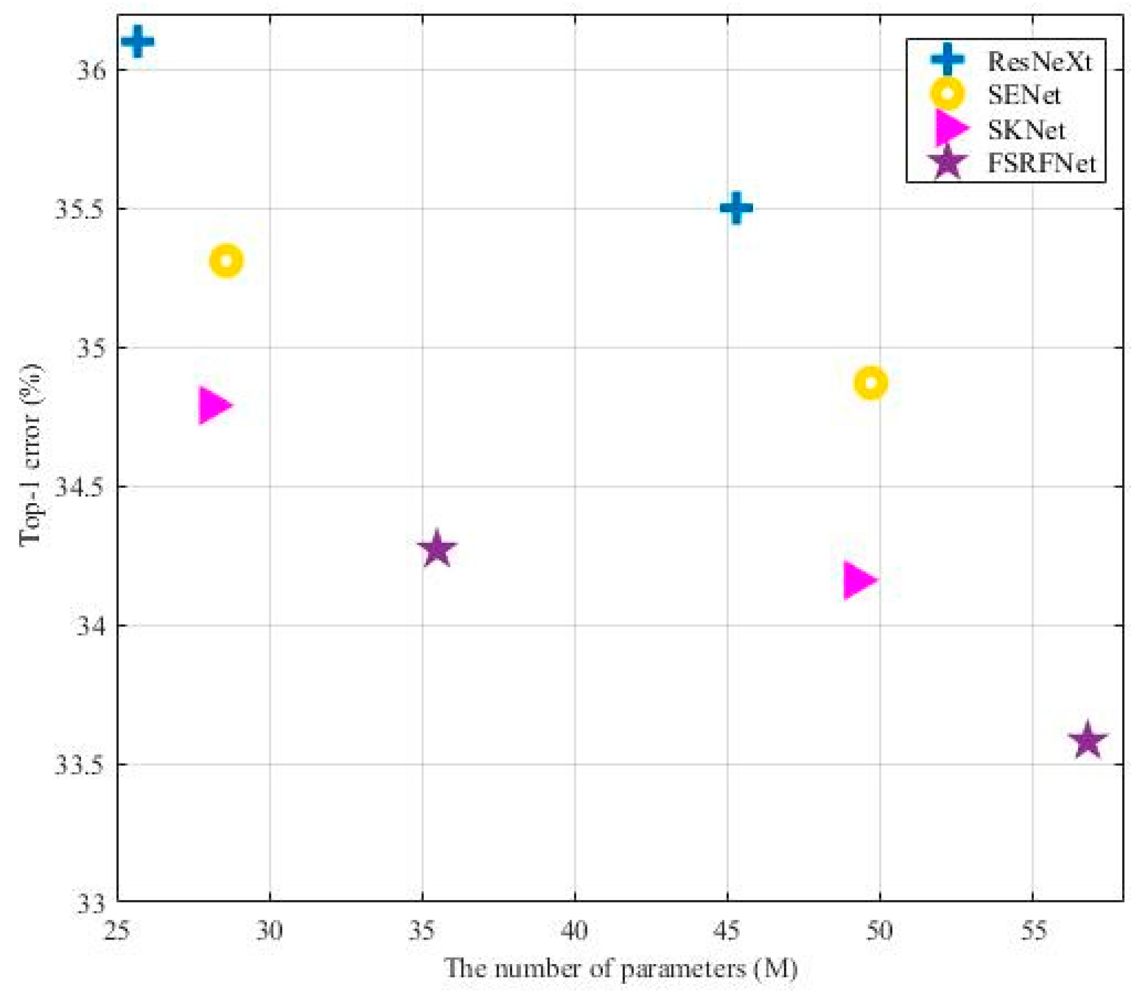
We begin by comparing FSRFNets to the public competitive models with different depths.

Table 2. Single 224 × 224 cropped top-1 error rates (%) on the Tiny ImageNet validation set and complexity comparisons. SENet, SKNet, and FSRFNet are all based on the corresponding ResNeXt backbones. The definition of FLOPs follows [56], i.e., the number of floating-point multiplication-adds. and #P denotes the number of parameters.

Models	#P	GFLOPs	Top-1 Err. (%)
ResNeXt-50 (our impl.)	25.7M	4.36	36.12
ResNeXt-101 (our impl.)	45.3M	8.07	35.54
SENet-50 (our impl.)	28.6M	4.51	35.31
SENet-101 (our impl.)	49.7M	8.13	34.87
SKNet-50 (our impl.)	28.1M	4.78	34.79
SKNet-101 (our impl.)	49.2M	8.45	34.16
FSRFNet-50 (ours)	35.5M	5.86	34.27
FSRFNet-101 (ours)	56.8M	11.32	33.58

and Figure 5 show the comparison results on the Tiny ImageNet [54] validation set. As the illustrations show, FSRFNet-50 and FSRFNet-101 improve the performance of state-of-the-art attention-based network models at different depths compared to models of similar complexity. FSRFNet-50 and FSRFNet-101 achieve performance improvements of 5.1% and 5.5% over ResNeXt-50 and ResNeXt-101, respectively. In addition, FSRFNet-50 and FSRFNet-101 achieve performance increases of 2.9% and 3.7% compared to SENet-50 and SENet-101, respectively. We note also that gains of 1.5% and 1.7% can be obtained for FSRFNet-50 and FSRFNet-101, compared to SKNet-50 and SKNet-101, respectively. Surprisingly, FSRFNet-50 is not only 1.27% higher than the absolute accuracy of ResNeXt-101, but the parameters and calculations of FSRFNet-50 are 22% and 27% smaller than ResNeXt-101, respectively, which demonstrates the superiority of the additive effects of feature-selective and spatial attention.

We plot the top-1 error rate of the proposed ResNeXt-50, ResNeXt-101, SENet-50, SENet-101 SKNet-50, SKNet-101, FSRFNet-50 and FSRFNet-101 with respect to the number of parameters in the Figure 5. we can also find that FSRFNets utilizes parameters more efficiently than these models. For instance, FSRFNet-50 outperforms ResNeXt-50 by achieving ∼34.3 top-1 error with similar model complexity. Remarkably, FSRFNet-50 achieves ∼20.2 top-1 error, although SENet-101 and SKNeXt-101 is 40.0% and 38.6% larger in parameter.

Additionally, we choose the representative compact architecture of ShuffleNetV2 [38] and MobileNetV2 [39], which represents one of the strongest lightweight models, to evaluate the generalization capabilities of FSRF blocks. For comparison, SE, SK and FSRF blocks are embedded in ShuffleNetV2 [38] and MobileNetV2 [39]. Similar to [56], the number of channels in each block is scaled to generate networks of different complexities, marked as 0.5×, 0.75×, and 1×.

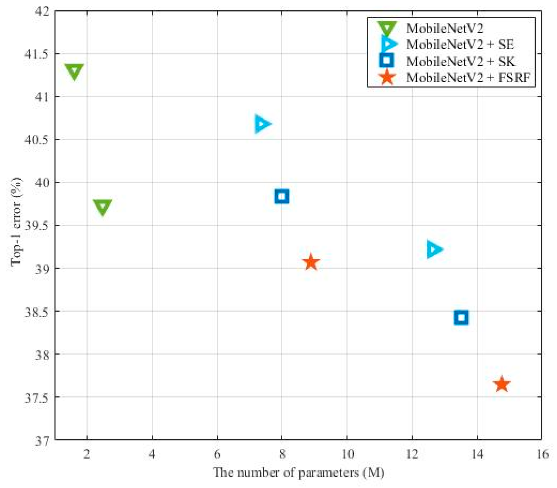
By exploring the different scale models in

Table 3. Single 224 × 224 cropped top-1 error rates (%) on the Tiny ImageNet validation set and complexity comparisons, with all models based on the corresponding ShuffleNetV2.

ShuffleNetV2	#P	MFLOPs	top-1 err. (%)
$0.5\times \left(\mathrm{our}\mathrm{impl}.\right)$	1.47M	37.62	47.82
$0.5\times +\mathrm{SE}\left(\mathrm{our}\mathrm{impl}.\right)$	1.59M	36.25	46.51
$0.5\times +\mathrm{SK}\left(\mathrm{our}\mathrm{impl}.\right)$	1.54M	38.78	45.01
$0.5\times +\mathrm{FSRF}\left(\mathrm{ours}\right)$	1.87M	40.41	43.33
$1.0\times \left(\mathrm{our}\mathrm{impl}.\right)$	2.35M	142.35	40.17
$1.0\times +\mathrm{SE}\left(\mathrm{our}\mathrm{impl}.\right)$	2.72M	140.93	38.64
$1.0\times +\mathrm{SK}\left(\mathrm{our}\mathrm{impl}.\right)$	2.67M	143.66	37.41
$1.0\times +\mathrm{FSRF}\left(\mathrm{ours}\right)$	3.23M	144.57	35.62

and

Table 4. Single 224 × 224 cropped top-1 error rates (%) on the Tiny ImageNet validation set and complexity comparisons, with all models based on the corresponding MobileNetV2.

MobileNetV2	#P	GFLOPs	top-1 err. (%)
$0.75\times \left(\mathrm{our}\mathrm{impl}.\right)$	1.61M	0.22	41.31
$0.75\times +\mathrm{SE}\left(\mathrm{our}\mathrm{impl}.\right)$	7.35M	1.61	40.68
$0.75\times +\mathrm{SK}\left(\mathrm{our}\mathrm{impl}.\right)$	8.01M	2.13	39.83
$0.75\times +\mathrm{FSRF}\left(\mathrm{ours}\right)$	8.89M	2.85	39.07
$1.0\times \left(\mathrm{our}\mathrm{impl}.\right)$	2.48M	0.31	39.73
$1.0\times +\mathrm{SE}\left(\mathrm{our}\mathrm{impl}.\right)$	12.63M	2.67	39.22
$1.0\times +\mathrm{SK}\left(\mathrm{our}\mathrm{impl}.\right)$	13.52M	3.54	38.43
$1.0\times +\mathrm{FSRF}\left(\mathrm{ours}\right)$	14.76M	4.36	37.65

, we can observe that FSRF blocks improve the accuracy based on ShuffleNetV2 [38] and MobileNetV2 [39] baselines. From Figure 6 and Figure 7, we can also see that FSRF blocks perform well compared to the ShuffleNetV2 [38] and MobileNetV2 [39] baseline models based on SENet and SKNet, respectively. The results show that $\mathrm{ShuffleNetV}2\_1.0\times +\mathrm{FSRF}$ performs well at ∼35.6 top-1 error level with comparable complexity than $\mathrm{ShuffleNetV}2\_1.0\times$, $\mathrm{ShuffleNetV}2\_1.0\times +\mathrm{SE}$ and $\mathrm{ShuffleNetV}2\_1.0\times +\mathrm{SK}$. Notably, we note that $\mathrm{MobileNetV}2\_0.75\times +\mathrm{FSRF}$ outperforms $\mathrm{MobileNetV}2\_1.0\times$ by above 0.66% accuracy, although $\mathrm{MobileNetV}2\_1.0\times$ is 25.7% larger in parameter.

5.2. CIFAR Classification

To further evaluate the performance of FSRFNets, we conduct experiments on CIFAR-10 and CIFAR-100 [57]. The CIFAR-10 [57] dataset consists of 60,000 $32\times 32$ color images in 10 classes, with 6000 images per class. There are 50,000 training images and 10,000 test images. The CIFAR-100 [57] dataset resembles the CIFAR-10 [57], except that it has 100 classes containing 600 images each. There are 500 training images and 100 testing images per class. The 100 classes in the CIFAR-100 [57] are grouped into 20 superclasses. Each image comes with a “fine” label (the class to which it belongs) and a “coarse” label (the superclass to which it belongs).

We use the same approach as above to integrate FSRF blocks into several popular baseline frameworks (ResNeXt-29 [9], ShuffleNetV2 [38], and MobileNetV2 [39]). Each baseline and its FSRFNet counterpart were trained using standard data enhancement strategies [58,59]. During the training process, the image is flipped horizontally, filled with four pixels on each side, and then randomly $32\times 32$ cropped. We report the performance of each baseline and its FSRFNet counterpart on CIFAR-10 and CIFAR-100 [57] in

Table 5. Top-1 errors (%) on CIFAR, with all models based on the corresponding ShuffleNetV2.

ShuffleNetV2	CIFAR-10	CIFAR-100
$0.5\times \left(\mathrm{our}\mathrm{impl}.\right)$	6.98	39.31
$0.5\times +\mathrm{SE}\left(\mathrm{our}\mathrm{impl}.\right)$	6.73	37.87
$0.5\times +\mathrm{SK}\left(\mathrm{our}\mathrm{impl}.\right)$	6.61	36.38
$0.5\times +\mathrm{FSRF}\left(\mathrm{ours}\right)$	6.46	34.64
$1.0\times \left(\mathrm{our}\mathrm{impl}.\right)$	6.29	33.24
$1.0\times +\mathrm{SE}\left(\mathrm{our}\mathrm{impl}.\right)$	6.17	32.32
$1.0\times +\mathrm{SK}\left(\mathrm{our}\mathrm{impl}.\right)$	5.93	30.71
$1.0\times +\mathrm{FSRF}\left(\mathrm{ours}\right)$	5.85	29.68

and

Table 6. Top-1 errors (%) on CIFAR, with SENet-29, SKNet-29, and FSRFNet-29 all based on ResNeXt-29, 16 × 32d.

Models	#P	CIFAR-10	CIFAR-100
$\mathrm{ResNeXt}-29,16\times 32\mathrm{d}\left(\mathrm{our}\mathrm{impl}.\right)$	24.5M	5.74	28.75
$\mathrm{ResNeXt}-29,8\times 64\mathrm{d}\left(\mathrm{our}\mathrm{impl}.\right)$	32.9M	5.58	28.37
$\mathrm{ResNeXt}-29,16\times 64\mathrm{d}\left(\mathrm{our}\mathrm{impl}.\right)$	66.7M	5.47	27.99
$\mathrm{SENet}-29\left(\mathrm{our}\mathrm{impl}.\right)$	34.1M	5.63	28.42
$\mathrm{SKNet}-29\left(\mathrm{our}\mathrm{impl}.\right)$	26.8M	5.42	27.68
$\mathrm{FSRFNet}-29\left(\mathrm{ours}\right)$	29.6M	5.26	27.51

. From the results, we can find that FSRFNets outperform the baseline architectures in every comparison, suggesting that the benefits of FSRF blocks are not confined to the Tiny ImageNet [54] dataset. Remarkably, FSRFNet-29 outperforms ResNeXt-29, 16×64d by above absolute 0.21% accuracy, and almost halves the number of parameters, which is extremely efficient. For Lightweight models, we compare FSRF blocks with the ShuffleNetV2 [38] and MobileNetV2 [39] baseline models based on SE blocks and SK blocks. $\mathrm{ShuffleNetV}2\_0.5\times +\mathrm{FSRF}$ and $\mathrm{ShuffleNetV}2\_1.0\times +\mathrm{FSRF}$ achieve better performance than other models with corresponding scaling.

5.3. Visualization with Grad-CAM

To intuitively understand the adaptive RF sizes of neurons through the additive effects of feature-selective and spatial attention of FSRFNet, we use the Grad-CAM method [60] to visualize the class activation mapping (CAM) of SKNet-50 and our proposed FSRFNet-50 backbone networks. In the visualization examples shown in Figure 8, the areas with light colors indicate that the current area has great influence on the classification result. SKNet achieves good results in multi-scale information selection. However, Since FSRFNet has stronger ability to adaptively select the appropriate convolution kernel size, the FSRFNet has activation maps that tend to cover the whole object. Finally, compared with SKNet, our FSRFNet has a better class activation maps.

6. Conclusions

In this paper, inspired by the additive effect of feature-selective and spatial attention on the receptive field sizes of the visual cortex neurons, we constructed the Feature-selective and Spatial Receptive (FSRF) block and inserted it into existing convolutional architecture to form the FSRFNet architecture. The FSRF block is implemented via three operations: Multi-branch Convolution, Fuse, and Interactions between Feature-selective and Spatial Attention. Fuse combines the results of multiple branches with different kernel sizes, and constructs attention building blocks (average and max channel; and average and max spatial), on which SoftMax and sigmoid operators are applied. Numerous experiments have demonstrated the effectiveness of FSRFNet from large models to small models and from large datasets to small datasets, including various benchmarks.

References

1. Simonyan, K.; Zisserman, A. Very deep convolutional networks for large-scale image recognition. arXiv 2014, arXiv:1409.1556. [Google Scholar]
2. Szegedy, C.; Liu, W.; Jia, Y.; Sermanet, P.; Reed, S.; Anguelov, D.; Rabinovich, A. Going deeper with convolutions. In Proceedings of the IEEE Conference on Computer Vision and Pattern Recognition, Boston, MA, USA, 7–12 June 2015; pp. 1–9. [Google Scholar]
3. Ioffe, S.; Szegedy, C. Batch normalization: Accelerating deep network training by reducing internal covariate shift. arXiv 2015, arXiv:1502.03167. [Google Scholar]
4. Szegedy, C.; Vanhoucke, V.; Ioffe, S.; Shlens, J.; Wojna, Z. Rethinking the inception architecture for computer vision. In Proceedings of the IEEE Conference on Computer Vision and Pattern Recognition, Las Vegas, NV, USA, 27–30 June 2016; pp. 2818–2826. [Google Scholar]
5. Szegedy, C.; Ioffe, S.; Vanhoucke, V.; Alemi, A.A. Inception-v4, Inception-ResNet and the impact of residual connections on learning. In Proceedings of the Thirty-First AAAI Conference on Artificial Intelligence, San Francisco, California, USA 4–9 February 2017. [Google Scholar]
6. He, K.; Zhang, X.; Ren, S.; Sun, J. Deep residual learning for image recognition. In Proceedings of the IEEE Conference on Computer Vision and Pattern Recognition, Las Vegas, NV, USA, 27–30 June 2016; pp. 770–778. [Google Scholar]
7. Zagoruyko, S.; Komodakis, N. Wide residual networks. arXiv 2016, arXiv:1605.07146. [Google Scholar]
8. Krizhevsky, A.; Sutskever, I.; Hinton, G.E. ImageNet classification with deep convolutional neural networks. In Proceedings of the Neural Information Processing Systems (NIPS), Harrahs and Harveys, Lake Tahoe, CA, USA, 3–8 December 2012; pp. 1097–1105. [Google Scholar]
9. Xie, S.; Girshick, R.; Dollár, P.; Tu, Z.; He, K. Aggregated residual transformations for deep neural networks. In Proceedings of the IEEE Conference on Computer Vision and Pattern Recognition, Honolulu, HI, USA, 21–26 July 2017; pp. 1492–1500. [Google Scholar]
10. Chollet, F. Xception: Deep learning with depthwise separable convolutions. In Proceedings of the IEEE Conference on Computer Vision and Pattern Recognition, Honolulu, HI, USA, 21–26 July 2017; pp. 1251–1258. [Google Scholar]
11. Howard, A.G.; Zhu, M.; Chen, B.; Kalenichenko, D.; Wang, W.; Weyand, T.; Adam, H. MobileNet: Efficient convolutional neural networks for mobile vision applications. arXiv 2017, arXiv:1704.04861. [Google Scholar]
12. Huang, G.; Liu, Z.; Van Der Maaten, L.; Weinberger, K.Q. Densely connected convolutional networks. In Proceedings of the IEEE Conference on Computer Vision and Pattern Recognition, Honolulu, HI, USA, 21–26 July 2017; pp. 4700–4708. [Google Scholar]
13. Girshick, R.; Donahue, J.; Darrell, T.; Malik, J. Rich feature hierarchies for accurate object detection and semantic segmentation. In Proceedings of the IEEE Conference on Computer Vision and Pattern Recognition, Columbus, OH, USA, 23–28 June 2014; pp. 580–587. [Google Scholar]
14. Uijlings, J.R.; van de Sande, K.E.; Gevers, T.; Smeulders, A.W. Selective search for object recognition. Int. J. Comput. Vis. 2013, 104, 154–171. [Google Scholar] [CrossRef]
15. Cortes, C.; Vapnik, V. Support vector networks. Mach. Learn. 1995, 20, 273–297. [Google Scholar] [CrossRef]
16. He, K.; Zhang, X.; Ren, S. Spatial Pyramid Pooling in Deep Convolutional Networks for Visual Recognition. IEEE Trans. Pattern Anal. Mach. Intell. 2015, 37, 1904–1916. [Google Scholar] [CrossRef] [PubMed] [Green Version]
17. Girshick, R. Fast r-cnn. Deformable part models are convolutional neural networks. In Proceedings of the IEEE Conference on Computer Vision, Boston, MA, USA, 8–10 June 2015; pp. 1440–1448. [Google Scholar]
18. Ren, S.; He, K.; Girshick, R. Faster r-cnn: Towards real-time object detection with region proposal networks. In Proceedings of the International Conference on Neural Information Processing Systems, Cambridge, MA, USA, 7–12 December 2015; pp. 91–99. [Google Scholar]
19. Redmon, J.; Divvala, S.; Girshick, R. You only look once: Unified, real-time object detection. In Proceedings of the IEEE Conference on Computer Vision and Pattern Recognition, Las Vegas, NV, USA, 27–30 June 2016; pp. 779–788. [Google Scholar]
20. Liu, W.; Anguelov, D.; Erhan, D.; Szegedy, C.; Reed, S.; Fu, C.Y.; Berg, A.C. SSD: Single Shot MultiBox detector. In Proceedings of the European Conference on Computer Vision, Amsterdam, The Netherlands, 8–16 October 2016; pp. 21–37. [Google Scholar]
21. Redmon, J.; Farhadi, A. Yolo 9000: Better, faster, stronger. In Proceedings of the IEEE Conference on Computer Vision and Pattern Recognition, Honolulu, HI, USA, 21–26 July 2017; pp. 6517–6525. [Google Scholar]
22. Redmon, J.; Farhadi, A. Yolo v3: An incremental improvement. arXiv 2018, arXiv:1804.02767. [Google Scholar]
23. Mnih, V.; Heess, N.; Graves, A. Recurrent models of visual attention. In Proceedings of the Neural Information Processing Systems (NIPS), Montréal, QC, Canada, 8–13 December 2014; pp. 2204–2212. [Google Scholar]
24. Xu, K.; Ba, J.; Kiros, R.; Cho, K.; Courville, A.; Salakhudinov, R.; Bengio, Y. Show, attend and tell: Neural image caption generation with visual attention. In Proceedings of the 32nd International Conference on Machine Learning, Lille, France, 6–11 July 2015; pp. 2048–2057. [Google Scholar]
25. Jaderberg, M.; Simonyan, K.; Zisserman, A. Spatial transformer networks. In Proceedings of the Neural Information Processing Systems (NIPS), Montréal, QC, Canada, 8–13 December 2015; pp. 2017–2025. [Google Scholar]
26. Hubel, D.H.; Wiesel, T.N. Receptive fields, binocular interaction and functional architecture in the cat’s visual cortex. J. Physiol. 1962, 160, 106–154. [Google Scholar] [CrossRef]
27. Desimone, R.; Wessinger, M.; Thomas, L.; Schneider, W. Attentional control of visual perception: Cortical and subcortical mechanisms. Cold Spring Harb. Symp. Quant. Biol. 1990, 55, 963–971. [Google Scholar] [CrossRef]
28. Nelson, J.I.; Frost, B.J. Orientation-selective inhibition from beyond the classic visual receptive field. Brain Res. 1978, 139, 359–365. [Google Scholar] [CrossRef]
29. Hayden, B.Y.; Gallant, J.L. Time course of attention reveals different mechanisms for spatial and feature-based attention in area V4. Neuron 2005, 47, 637–643. [Google Scholar] [CrossRef]
30. Egner, T.; Monti, J.M.; Trittschuh, E.H.; Wieneke, C.A.; Hirsch, J.; Mesulam, M.M. Neural integration of top-down spatial and feature-based information in visual search. J. Neurosci. 2008, 28, 6141–6151. [Google Scholar] [CrossRef]
31. Andersen, S.K.; Fuchs, S.; Müller, M.M. Effects of feature-selective and spatial attention at different stages of visual processing. J. Cogn. Neurosci. 2011, 23, 238–246. [Google Scholar] [CrossRef]
32. Ibos, G.; Freedman, D.J. Interaction between spatial and feature attention in posterior parietal cortex. Neuron 2016, 91, 931–943. [Google Scholar] [CrossRef]
33. Li, X.; Wang, W.; Hu, X.; Yang, J. Selective Kernel Networks. In Proceedings of the IEEE Conference on Computer Vision and Pattern Recognition, Seattle, WA, USA, 15–21 July 2019; pp. 510–519. [Google Scholar]
34. Dudczyk, J. Radar emission sources identification based on hierarchical agglomerative clustering for large data sets. J. Sens. 2016, 2016, 1879327. [Google Scholar] [CrossRef]
35. Matuszewski, J. Radar signal identification using a neural network and pattern recognition methods. In Proceedings of the 14th International Conference on Advanced Trends in Radioelectionics, Telecommunications and Computer Engineering (TCSET 2018), Lviv-Slavsk, Ukraine, 20–24 February 2018; pp. 79–83. [Google Scholar] [CrossRef]
36. Dudczyk, J.; Wnuk, M. The utilization of unintentional radiation for identification of the radiation sources. In Proceedings of the 34 European Microwave Conference (EuMC 2004), Amsterdam, The Netherlands, 12–14 October 2004; Volume 2, pp. 777–780. [Google Scholar]
37. Matuszewski, J.; Pietrow, D. Recognition of electromagnetic sources with the use of deep neural networks. In Proceedings of the XII Conference on Reconnaissance and Electronic Warfare Systems, Oltarzew, Poland, 19–21 November 2018. [Google Scholar] [CrossRef]
38. Ma, N.; Zhang, X.; Zheng, H.T.; Sun, J. ShuffleNet v2: Practical guidelines for efficient CNN architecture design. In Proceedings of the European Conference on Computer Vision, Munich, Germany, 8–14 September 2018; pp. 116–131. [Google Scholar]
39. Sandler, M.; Howard, A.; Zhu, M.; Zhmoginov, A.; Chen, L.C. MobileNet v2: Inverted residuals and linear bottlenecks. In Proceedings of the IEEE Conference on Computer Vision and Pattern Recognition, Salt Lake City, UT, USA, 18–22 June 2018; pp. 4510–4520. [Google Scholar]
40. Long, J.; Shelhamer, E.; Darrell, T. Fully convolutional networks for semantic segmentation. In Proceedings of the IEEE Conference on Computer Vision and Pattern Recognition, Boston, MA, USA, 7–12 June 2015; pp. 3431–3440. [Google Scholar]
41. Itti, L.; Koch, C. Computational modelling of visual attention. Nat. Rev. Neurosci. 2001, 2, 194–203. [Google Scholar] [CrossRef] [Green Version]
42. Itti, L.; Koch, C.; Niebur, E. A model of saliency-based visual attention for rapid scene analysis. IEEE Trans. Pattern Anal. Mach. Intell. 1998, 20, 1254–1259. [Google Scholar] [CrossRef] [Green Version]
43. Larochelle, H.; Hinton, G.E. Learning to combine foveal glimpses with a third-order Boltzmann machine. In Proceedings of the Neural Information Processing Systems (NIPS), Vancouver, WA, Canada, 6–11 December 2010; pp. 1243–1251. [Google Scholar]
44. Bahdanau, D.; Cho, K.; Bengio, Y. Neural machine translation by jointly learning to align and translate. arXiv 2014, arXiv:1409.0473. [Google Scholar]
45. You, Q.; Jin, H.; Wang, Z.; Fang, C.; Luo, J. Image captioning with semantic attention. In Proceedings of the IEEE Conference on Computer Vision and Pattern Recognition, Las Vegas, NV, USA, 27–30 June 2016; pp. 4651–4659. [Google Scholar]
46. Chung, J.S.; Senior, A.; Vinyals, O.; Zisserman, A. Lip reading sentences in the wild. In Proceedings of the IEEE Conference on Computer Vision and Pattern Recognition, Honolulu, HI, USA, 21–26 July 2017; pp. 3444–3453. [Google Scholar]
47. Wang, F.; Jiang, M.; Qian, C.; Yang, S.; Li, C.; Zhang, H.; Tang, X. Residual attention network for image classification. In Proceedings of the IEEE Conference on Computer Vision and Pattern Recognition, Honolulu, HI, USA, 21–26 July 2017; pp. 3156–3164. [Google Scholar]
48. Woo, S.; Park, J.; Lee, J.Y.; Kweon, I.S. CBAM: Convolutional Block Attention Module. In Proceedings of the European Conference on Computer Vision, Munich, Germany, 8–14 September 2018; pp. 3–19. [Google Scholar]
49. Motter, B.C. Focal attention produces spatially selective processing in visual cortical areas V1, V2, and V4 in the presence of competing stimuli. J. Neurophysiol. 1993, 70, 909–919. [Google Scholar] [CrossRef]
50. Luck, S.J.; Chelazzi, L.; Hillyard, S.A.; Desimone, R. Neural mechanisms of spatial selective attention in areas V1, V2, and V4 of macaque visual cortex. J. Neurophysiol. 1997, 77, 24–42. [Google Scholar] [CrossRef]
51. Kastner, S.; Ungerleider, L.G. Mechanisms of visual attention in the human cortex. Annu. Rev. Neurosci. 2000, 23, 315–341. [Google Scholar]
52. Chawla, D.; Lumer, E.D.; Friston, K.J. The relationship between synchronization among neuronal populations and their mean activity levels. Neural Comput. 1999, 11, 1389–1411. [Google Scholar] [CrossRef]
53. Bartsch, M.V.; Donohue, S.E.; Strumpf, H.; Schoenfeld, M.A.; Hopf, J.M. Enhanced spatial focusing increases feature-based selection in unattended locations. Sci. Rep. 2018, 8, 16132:1–16132:14. [Google Scholar] [CrossRef]
54. Yao, L.; Miller, J. Tiny imagenet classification with convolutional neural networks. CS 231N. 2015, 2, 8. [Google Scholar]
55. He, K.; Zhang, X.; Ren, S.; Sun, J. Delving deep into rectifiers: Surpassing human-level performance on ImageNet classification. In Proceedings of the IEEE Conference on Computer Vision, Boston, MA, USA, 7–12 June 2015; pp. 1026–1034. [Google Scholar]
56. Zhang, X.; Zhou, X.; Lin, M.; Sun, J. Shufflenet: An extremely efficient convolutional neural network for mobile devices. In Proceedings of the IEEE International Conference on Computer Vision, Salt Lake City, UT, USA, 18–22 June 2018; pp. 6848–6856. [Google Scholar]
57. Krizhevsky, A.; Hinton, G. Learning Multiple Layers of Features from Tiny Images (Technical Report); University of Toronto: Toronto, ON, Canada, 2009; Volume 1. [Google Scholar]
58. Lin, M.; Qiang, C.; Shuicheng, Y. Network in network. arXiv 2013, arXiv:1312.4400. [Google Scholar]
59. Huang, G.; Sun, Y.; Liu, Z.; Sedra, D.; Weinberger, K.Q. Deep networks with stochastic depth. In Proceedings of the European Conference on Computer Vision, Amsterdam, The Netherlands, 8–16 October 2016; pp. 646–661. [Google Scholar]
60. Selvaraju, R.R.; Cogswell, M.; Das, A.; Vedantam, R.; Parikh, D.; Batra, D. Grad-cam: Visual explanations from deep networks via gradient-based localization. In Proceedings of the IEEE International Conference on Computer Vision, Honolulu, HI, USA, 21–26 July 2017; pp. 618–626. [Google Scholar]
Figure 1. The structure of the “Feature-selective and Spatial Receptive Fields” (FSRF) block.
Applsci 09 03954 g001
Figure 2. The structure of the average and max channel (AMC) attention building block.
Applsci 09 03954 g002
Figure 3. The structure of the average and max spatial (AMS) attention building block.
Applsci 09 03954 g003
Figure 4. The schema of an FSRF-ResNet module.
Applsci 09 03954 g004
Figure 5. Relationship between the performance of FSRFNet and the number of its parameters, compared with the corresponding ResNeXt backbones.
Applsci 09 03954 g005
Figure 6. Relationship between performance and the number of parameters: FSRFNet compared with the corresponding lightweight model ShuffleNetV2.
Applsci 09 03954 g006
Figure 7. Relationship between performance and the number of parameters: FSRFNet compared with the corresponding lightweight model MobileNetV2.
Applsci 09 03954 g007
Figure 8. The Grad-CAM visualization results, using SKNet-50 and our proposed FSRFNet-50 as backbone networks.
Applsci 09 03954 g008