Article

Impact of Wind on the Movement of the Load Carried by Rotary Crane

1
Institute of Mechanics and Machine Design Fundamentals, Czestochowa University of Technology, 42-201 Czestochowa, Poland
2
Institute of Thermal Machinery, Czestochowa University of Technology, 42-201 Czestochowa, Poland
*
Author to whom correspondence should be addressed.
Appl. Sci. 2019, 9(18), 3842; https://doi.org/10.3390/app9183842
Submission received: 4 August 2019 / Revised: 30 August 2019 / Accepted: 3 September 2019 / Published: 12 September 2019
(This article belongs to the Section Mechanical Engineering)

Abstract

:
This paper considers the coupled kinematic and dynamic models of a mobile crane. A full description of boom and load movement has been provided as a response of the system to the influence of kinematic forces. The linear system model was treated as rigid, and the carried load as a nondeformed static body. To describe the position of said load, Bryant angles were used. The dynamic model includes the impact of external forces (wind pressure) while load carrying and positioning. Algorithm and calculation software were developed to enable dynamic phenomena analysis during both a work cycle and free movement of said load. The initial problem was solved by means of the ode45 calculation procedure in the Matlab software based on the Runge–Kutta 4th Order Method. The work presents exemplary results of load movement simulation with respect to various wind velocities, selected on the basis of guidelines from Poland’s standards regarding safe operation of mechanical equipment.

1. Introduction

The truck crane is currently one of the most important modes of equipment transport used to enable handling and assembly. Technological development and the increase of computational capabilities of computers allows comprehensive analysis of a modelling problem, which has a crucial impact on the design stage of new structures or during modification of existing objects. The literature on the subject lists a series of works pertaining to the problem of modelling crane dynamics; optimization of their work cycles; or influence of external forces. The problem of crane dynamics with the inclusion of various load transportation processes was presented in Works [1,2,3]. Paper [1] presents a dynamic model of a mobile crane and a carried load in which the flexibility of the support system was taken into account. The impact of the support system model on mobile crane stability was also analyzed. Paper [2] deals with the problem of dynamic analysis of a rotary crane with a description of all work stages (i.e., lifting, transport, and reloading of load). In addition, the article provides the mechanical–mathematical model with the use of Lagrange’s equation of the second order. In Work [3], the theoretical and computational model of a forest crane and carried loads was presented. The numerical program, which has been developed in this work, allows analysis of load motion resulting from a crane’s operating mechanism. The simulation model of a crane with the assurance of its stability was considered in Works [4,5,6,7]. Paper [4] presents a stability assessment method of a truck crane’s handling system and trajectory optimization process where safety indicator values were accepted as the criterion. Article [5] deals with the determination of a truck crane’s outrigger reaction and stability factor monitoring during lift operations. In Paper [6], the mathematical model of the control system for a mobile crane was presented. Numerical analyses with multiple strategies of rotational motion control and different types of controllers were also conducted. Moreover, the experimental results were discussed. The inherent stability of nonslewing articulated mobile cranes (NSAM) was analyzed in Work [7]. Different configurations and design geometry of the NSAM were checked. Papers [8,9] present a dynamic analysis of particular elements of a mobile crane [8] and a harbor crane [9] together with the damping of those systems. Work [9] also performs a sensitivity analysis by tornado diagram and fast nonlinear analysis of container cranes. The influence of external forces, having impact on load-carrying systems was analyzed, inter alia, in Works [10,11,12]. In Paper [11], wind power impact on a container crane located in atmospheric boundary layers was considered, where wind power was measured with the use of a seven-component balance with different wind directions. The problem of positioning, work cycle optimization, and development of monitoring systems for a carried load were presented in Papers [6,13,14,15,16,17,18]. In the optimization process, new technological approaches were used (i.e., LiDAR scanner [13], three-dimensional (3D) visualization [15], or fuzzy-set logic models [19]). The influence of crane component flexibilities was also analyzed in Works [16,17].
This work presents a dynamic model of the system: truck crane—carried load. Dynamic problems were considered concerning two coupled planes of movement (lifting and rotation) with the inclusion of kinematic dependencies of the real system.

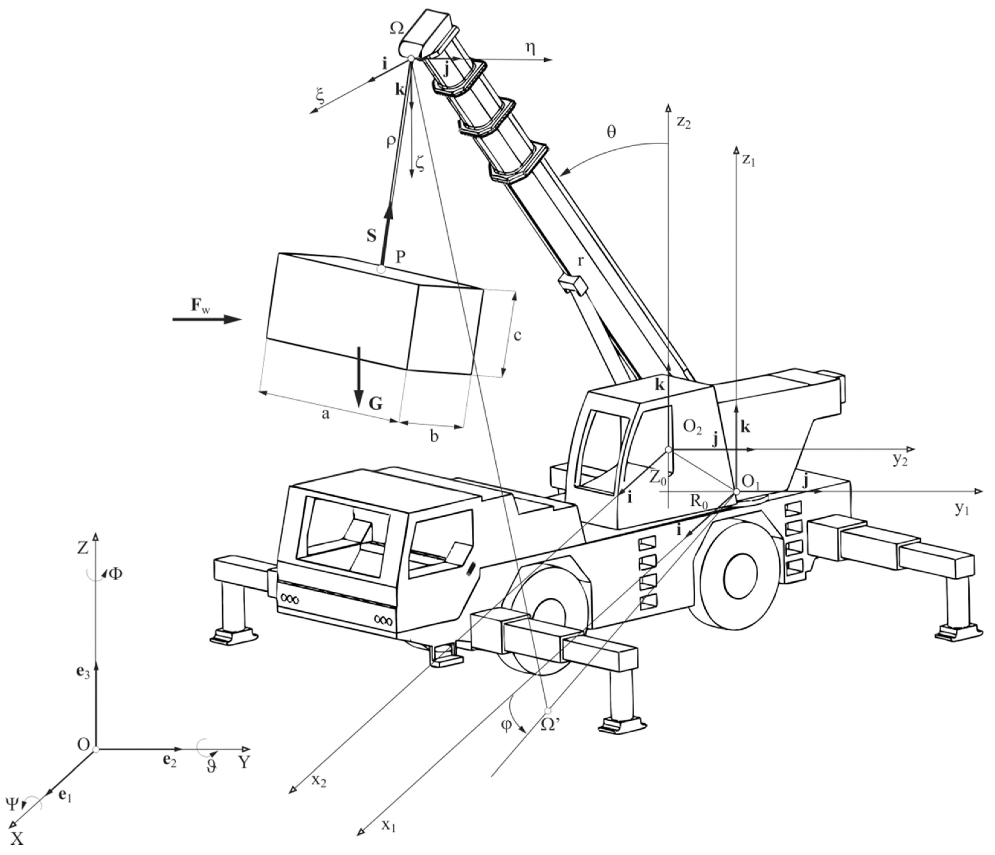
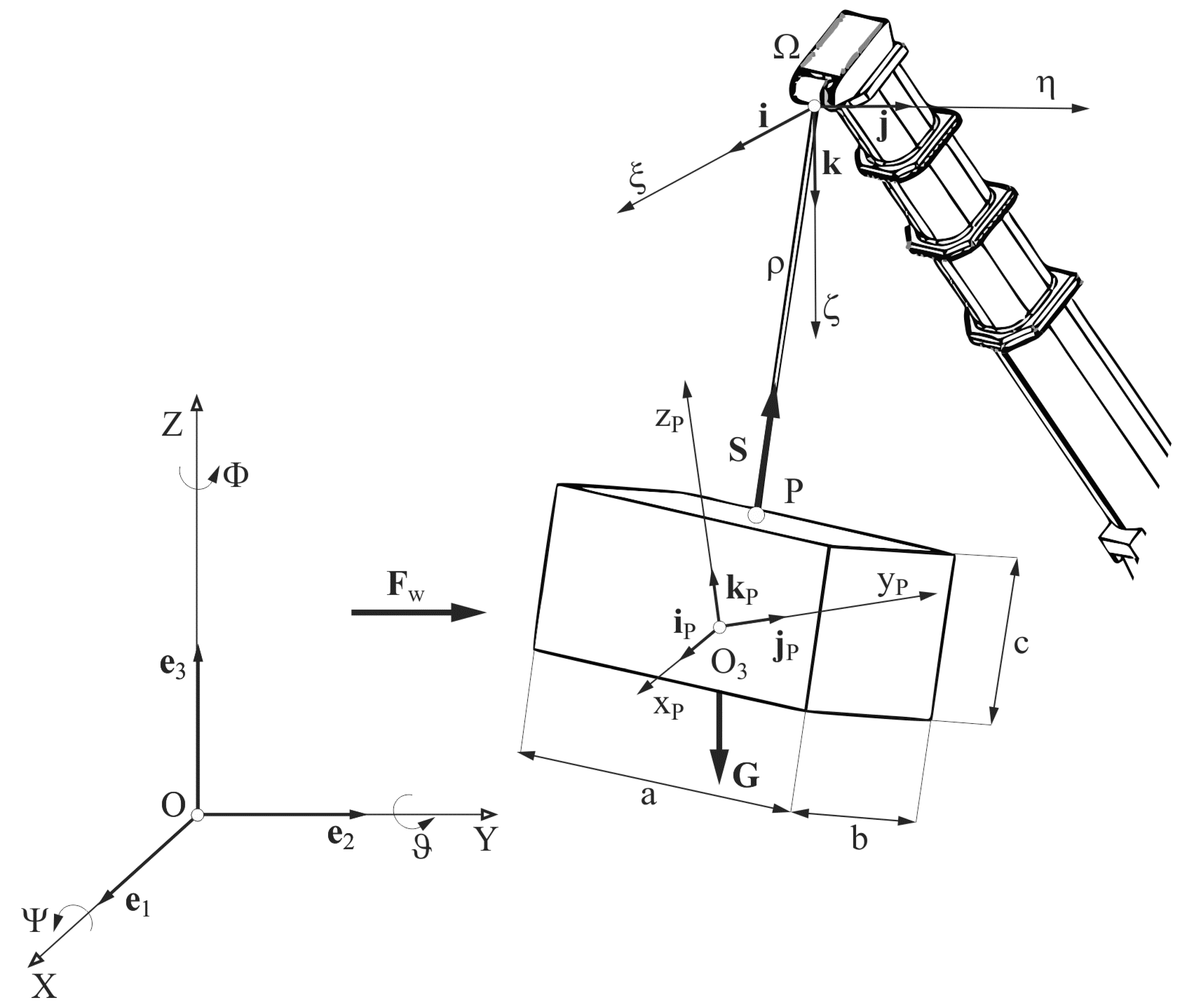
2. Model of the Studied System

The model of the analyzed system (Figure 1) was developed based on a real object. The computational model may be divided into two coupled parts: kinematic—where movement parameters of the studied system were determined and dynamic—and the response of the system to kinematic forces.
In the present paper, the coupled kinematic and dynamic models were developed according to certain assumptions [1,16]. The kinematic aspect concerns the analysis of a two-member telescopic boom and pulley system of a truck crane. The dynamic part, as well as wind influence, is related to the movement of the load. The influence of wind force on boom dynamics has not been taken into account. The main systems of the rotary crane were treated as rigid bodies, and the mobile crane was set on a rigid base. The boom of the crane was treated as a beam with infinite stiffness and variable length. The load was treated as a stable, static body attached at point Ω on a nondeformable cable having variable length resulting from the work of the winch, boom movement, and extension. The direction of wind power impact was adopted as constant and acting following the directions of the X or Y axes of the global coordinate system.
Due to the adopted assumptions, the following rectangular systems were introduced: O1x1y1z1—the inertial system connected with the chassis of the crane; O2x2y2z2—the movable system connected with the point of the boom’s support in the crane body; Ωξηζ—the movable system connected with the boom tip (point Ω); and OXYZ—the movable system connected with the load. Additionally, two systems of curvilinear coordinates were introduced: cylindrical coordinates R, α, Z in the system O1x1y1z1, and spherical coordinates r, θ, φ in the system O2x2y2z2.
The kinematic problems of truck cranes were further described in Works [1,18], where the kinematics of point Ω were presented. The control of this type of system takes place through changes of the following coordinates: r—boom length, θ—boom inclination angle, φ and α (where α = φ + π)—boom and crane body rotation angles. The movement of the load is a composition of the boom tip movement Ω and the center of mass of the carried load, which is dependent on the change of cable length coordinate ρ, presented by the generalized coordinates as ρ2 = ξ2 + η2 + ζ2.

3. Equations of Motion for the Studied System

The general movement of the rigid body may be presented as a connection of translational motion, in relation to the beginning of the global coordinate system, and rotational motion, in relation to the center of load mass. The rotation of the local coordinate system connected with the load in relation to the global system may be defined by means of Bryant angles. The vector components of angular velocity, using Bryant angles, may be presented in the form of [12]:
ω x ω 1 = Ψ ˙ cos ϑ cos Φ + ϑ ˙ sin Φ , ω y ω 2 = Ψ ˙ cos ϑ sin Φ + ϑ ˙ cos Φ , ω z ω 3 = Ψ ˙ sin ϑ + Φ ˙ ,
where Ψ, ϑ and Φ are the Bryant angles.
The components of the angular acceleration vector can be determined by differentiation of dependence (1):
ε x = Ψ ¨ cos ( ϑ ) cos ( Φ ) ϑ ¨ sin ( Φ ) Ψ ˙ Φ ˙ sin ( Φ ) cos ( ϑ ) + Ψ ˙ ϑ ˙ cos ( Φ ) sin ( ϑ ) Φ ˙ ϑ ˙ cos ( Φ ) , ε y = Ψ ¨ cos ( ϑ ) sin ( Φ ) + ϑ ¨ cos ( Φ ) + Ψ ˙ Φ ˙ cos ( Φ ) cos ( ϑ ) + + Ψ ˙ ϑ ˙ sin ( Φ ) sin ( ϑ ) Φ ˙ ϑ ˙ sin ( Φ ) , ε z = Ψ ¨ sin ( ϑ )   + Φ ¨ Ψ ˙ ϑ ˙ cos ( ϑ ) .
The movable systems of rectangular coordinates were adopted in such a manner that respective axes thereof remain parallel with respect to each other. Therefore, relative movements of the systems are translational motions [1].

3.1. Equations of Motion of the Main System

The movement of the load as the movement of a rigid body is described by the system of two vector equations [3,20,21]:
{ (3a) m a C = F C , (3b) d d t K C = M C ,
where m is the mass of the carried load, aC is the absolute translational acceleration vector of the load’s center of mass in the global coordinate system, FC is the resultant vector of all the forces acting on said load, KC is the angular momentum vector of the load in relation to its center of mass, and MC is the moment vector from all the forces acting on the load in relation to the center of mass.
By taking into consideration the angular velocity vector ωC and the matrix of inertia moments Jc, it is possible to record the vector of the load’s angular momentum in relation to its center of mass:
K C = J C ω C
including the total angular momentum derivative of the body in the fixed system
d d t K C = d d t K C + ω C × K C ,
rotational motion (3b), using the Einstein summation convention, can be described as [16]:
M j = J j m ε m + ε j k m ω k J m n ω n , j = 1 , 2 , 3 ,
where εjkm is the Levi–Civita permutation symbol.
By not including air resistances to motion, the resultant force vector FC constitutes the vector sum of the tension in cable S, load gravity force G, and the impact of external forces Fw:
F C = S + G + F w .
By conducting the projection of forces in the global coordinate system
S = ( S ξ i + S η j S ζ k ) , G = m g k , F w = F w x i + F w y j + F w z k ,
and presenting the acceleration vector aC as the sum of the boom tip component acceleration including the center of load mass:
a C x = a Ω x + ξ ¨ , a C y = a Ω y + η ¨ , a C z = a Ω z + g ζ ¨ ,
it is possible to depict the vector Equation (3a) in the following manner:
{ m ( a Ω x + ξ ¨ ) + S ξ + F w x = 0 , m ( a Ω y + η ¨ ) + S η + F w y = 0 , m ( a Ω z + g ζ ¨ ) S ζ + F w z = 0 ,
which, after certain transformations, may be presented as [1,20]:
ξ ¨ = a Ω x + F w x m + ξ ρ 2 [ ρ ρ ¨ + ρ ˙ 2 + ξ a Ω x + η a Ω y ζ ( a Ω z + g ) ( ξ ˙ 2 + η ˙ 2 + ζ ˙ 2 ) ] , η ¨ = a Ω y + F w y m + η ρ 2 [ ρ ρ ¨ + ρ ˙ 2 + ξ a Ω x + η a Ω y ζ ( a Ω z + g ) ( ξ ˙ 2 + η ˙ 2 + ζ ˙ 2 ) ] , ζ ¨ = a Ω z + g + F w z m + ζ ρ 2 [ ρ ρ ¨ + ρ ˙ 2 + ξ a Ω x + η a Ω y ζ ( a Ω z + g ) ( ξ ˙ 2 + η ˙ 2 + ζ ˙ 2 ) ] .
Individual members of the boom tip acceleration (point Ω) can be written as [1]:
a Ω x = ( R 0 φ ˙ 2 ) cos φ + ( R 0 φ ¨ ) sin φ + ( r ¨ r θ ˙ 2 r φ ˙ 2 sin 2 θ ) sin θ cos φ + + ( r θ ¨ + 2 r ˙ θ ˙ r φ ˙ 2 sin θ cos θ ) cos θ cos φ [ r φ ¨ sin θ + 2 φ ˙ ( r ˙ sin θ + r θ ˙ cos θ ) ] sin φ , a Ω y = ( R 0 φ ˙ 2 ) sin φ ( R 0 φ ¨ ) cos φ + ( r ¨ r θ ˙ 2 r φ ˙ 2 sin 2 θ ) sin θ sin φ + + ( r θ ¨ + 2 r ˙ θ ˙ r φ ˙ 2 sin θ cos θ ) cos θ sin φ + [ r φ ¨ sin θ + 2 φ ˙ ( r ˙ sin θ + r θ ˙ cos θ ) ] cos φ , a Ω z = ( r ¨ r θ ˙ 2 r φ ˙ 2 sin 2 θ ) cos θ ( r θ ¨ + 2 r ˙ θ ˙ r φ ˙ 2 sin θ cos θ ) sin θ .
The impact of external forces (wind pressure) Fw may be shown as [22,23]:
F w = 1 2 ρ a i r A V 2 C D ,
where A—the area on which the force is acting, V—wind velocity, CD—aerodynamic resistance coefficient, and ρair—air density.
By including the above-mentioned dependencies, a system of six ordinary differential equations of the 2nd order are obtained which, after certain transformations, may be presented as [1]:
D ji X ¨ j = E i ,
where the coefficient of matrix Dji and vector Ei depend only on functions X i and X ˙ including the functions controlling the system (r, θ, φ and ρ).
In order to solve the initial problem of load motion, the system of Equations (14) should be reduced to a system of differential equations of the 1st order [24].

3.2. Initial Problem of Load Motion

In this paper, the coordinates r, θ, φ, and ρ were given as kinematic forces. As a result of solving the initial problem, it is possible to determine the functions describing the coordinates of load position ξ, η, ζ and its rotation angles Ψ, ϑ, Φ. As a result, it fully describes the behavior of the crane together with the carried load during the work cycle of the system.
In order to fully formulate the initial problem of system movement, it was necessary to supplement the formulation of the motion equation with the initial conditions that may be provided in the form:
ξ ( t ) | t = 0 = ξ 0 , ξ ˙ ( t ) | t = 0 = ξ ˙ 0 , η ( t ) | t = 0 = η 0 , η ˙ ( t ) | t = 0 = η ˙ 0 , ζ ( t ) | t = 0 = ζ 0 , ζ ˙ ( t ) | t = 0 = ζ ˙ 0 , Ψ ( t ) | t = 0 = Ψ 0 , Ψ ˙ ( t ) | t = 0 = Ψ ˙ 0 , Θ ( t ) | t = 0 = Θ 0 , Θ ˙ ( t ) | t = 0 = Θ ˙ 0 , Φ ( t ) | t = 0 = Φ 0 , Φ ˙ ( t ) | t = 0 = Φ ˙ 0 .
In order to solve the initial problem of motion, the ode45 calculation procedure, based on the Runge–Kutta 4th Order Method, was used in the Matlab environment [24,25]. The calculation was made with a variable integration step limited by tolerances: relative and absolute. The upper bound on ODE (Ordinary Differential Equations) solver step size was set to 1e-3s.

3.3. Variability of the Area on Which Wind Power Has Influence

In Equation (13), defining the impact of wind power, area A, on which the force has influence, is often treated as a constant value resulting from the initial position of the load [12,26]. The present paper includes the change of the area caused by both wind power and particular movements of crane’s elements, as well as defines the parameter of the effective area Aeff.
In order to determine the parameter Aeff, dependencies between the normal vectors of particular surfaces and the change of coordinates of three vertices of each analyzed surface were used.
By using the coordinates of three points (vertices): P1 = (x1,y1,z1), P2 = (x2,y2,z2), P3 = (x3,y3,z3), it is possible to determine the plane passing through these points, which may be presented by means of Equation [27]:
| X x 1 Y y 1 Z z 1 x 2 x 1 y 2 y 1 z 2 z 1 x 3 x 1 y 3 y 1 z 3 z 1 | = 0 .
Parameters of the general equation of this plane
α X + β Y + γ Z + μ = 0 ,
constitute component elements of the normal vector
n 1 = [ α i β i γ i ] .
By determining the normal vector of the plane, where wind power has influence
n 2 = [ 1 0 0 ] ,
it is possible to determine the angle measure between the normal vectors n1 and n2.
cos κ i = n 1 n 2 | n 1 | | n 2 | .
Subsequently, the parameter of the effective area on which wind power has an impact may be depicted as
A e f f = a b cos ( κ 1 ) + a c cos ( κ 2 ) + b c cos ( κ 3 ) ,
where a—length, b—width, and c—height of the carried load, and κ 1 , κ 2 as well as κ 3 are the angles between the normal vectors of particular surfaces.

4. Results and Discussion

In this work, two cases of load movement were analyzed. The first case, which was used to verify the calculation model, concerned a stationary telescopic boom. Such a motion can be treated as a mathematical pendulum movement. In this case, the motion was caused by an appropriate selection of initial conditions. The second case concerned the crane’s work under the influence of kinematic forces resulting from the crane’s working cycle. The parameters of the calculation model and the properties of the carried load are presented in Table 1. For every movement variant, various wind velocities were analyzed in accordance with the safety requirements of Poland’s standards for crane operation.

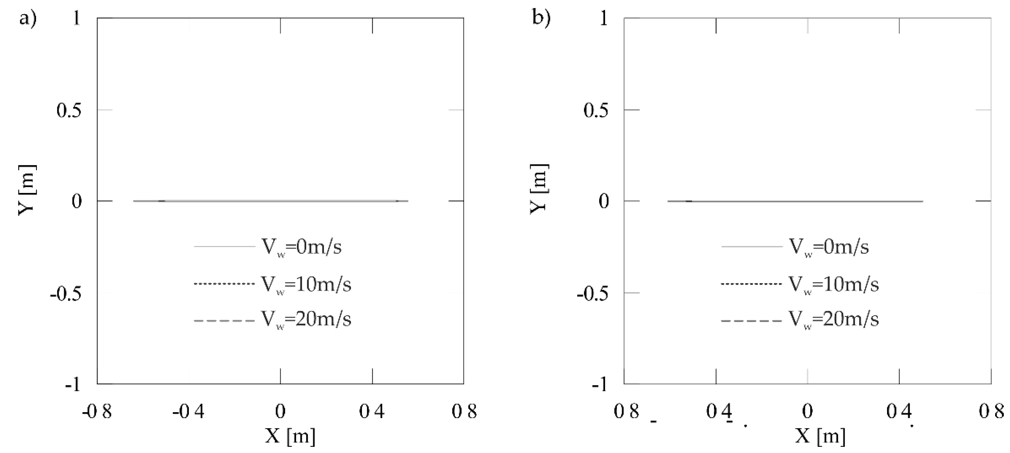
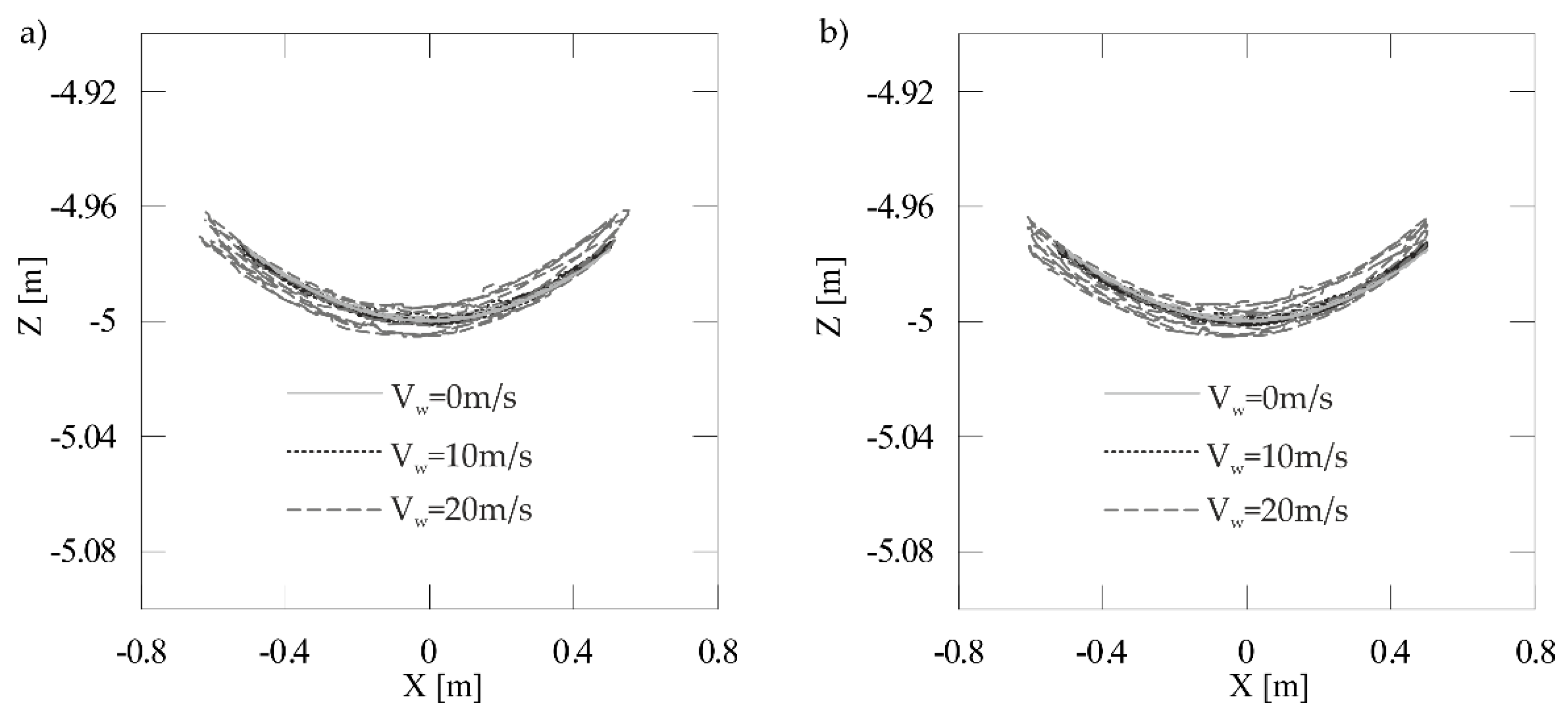
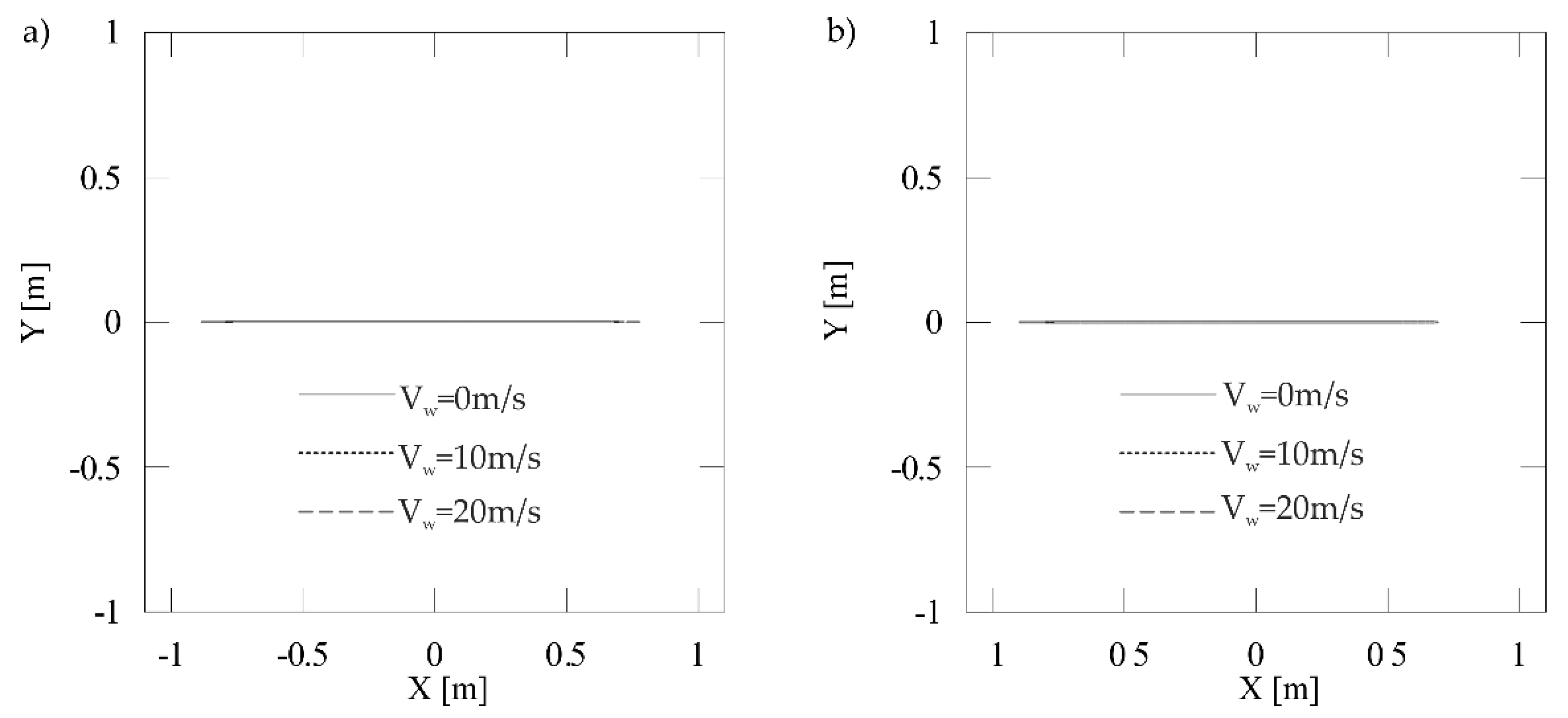
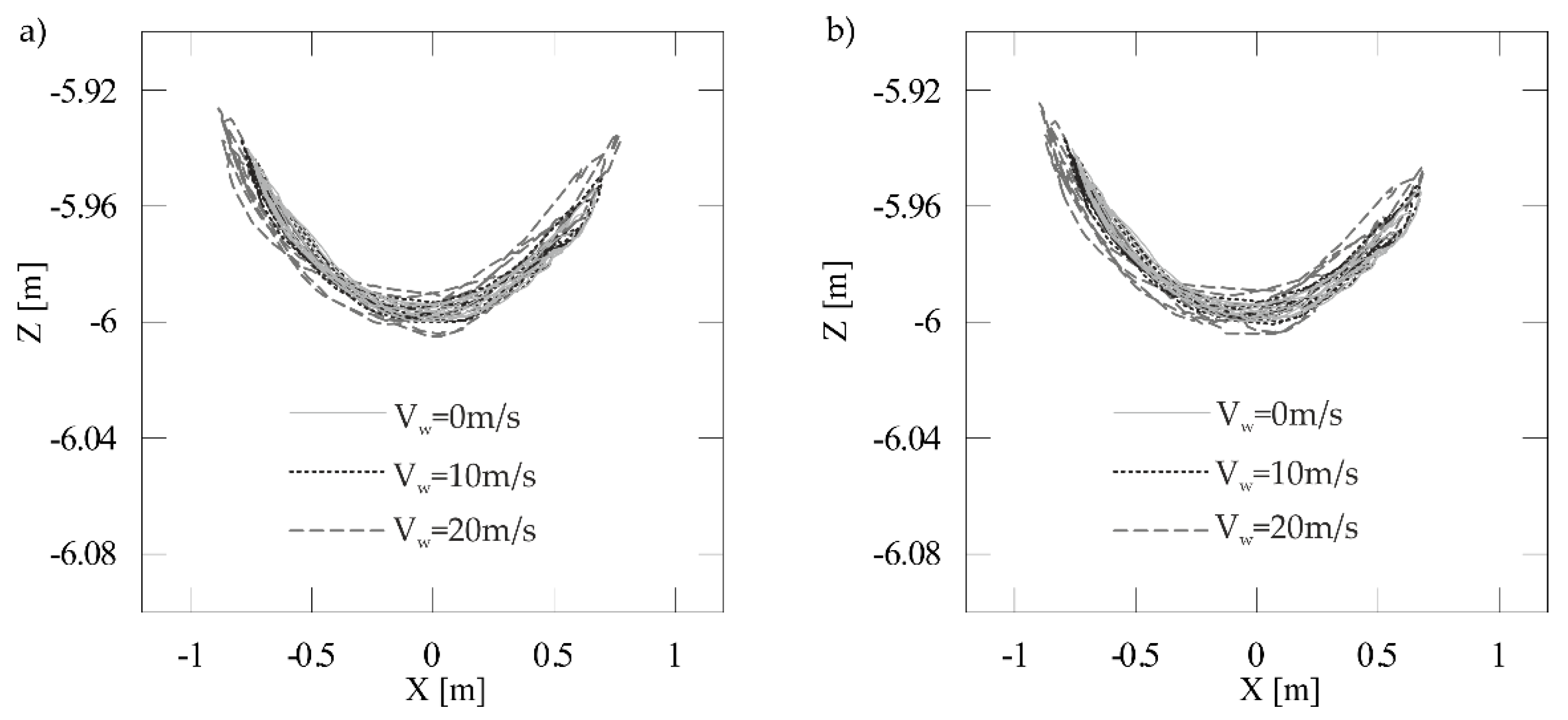
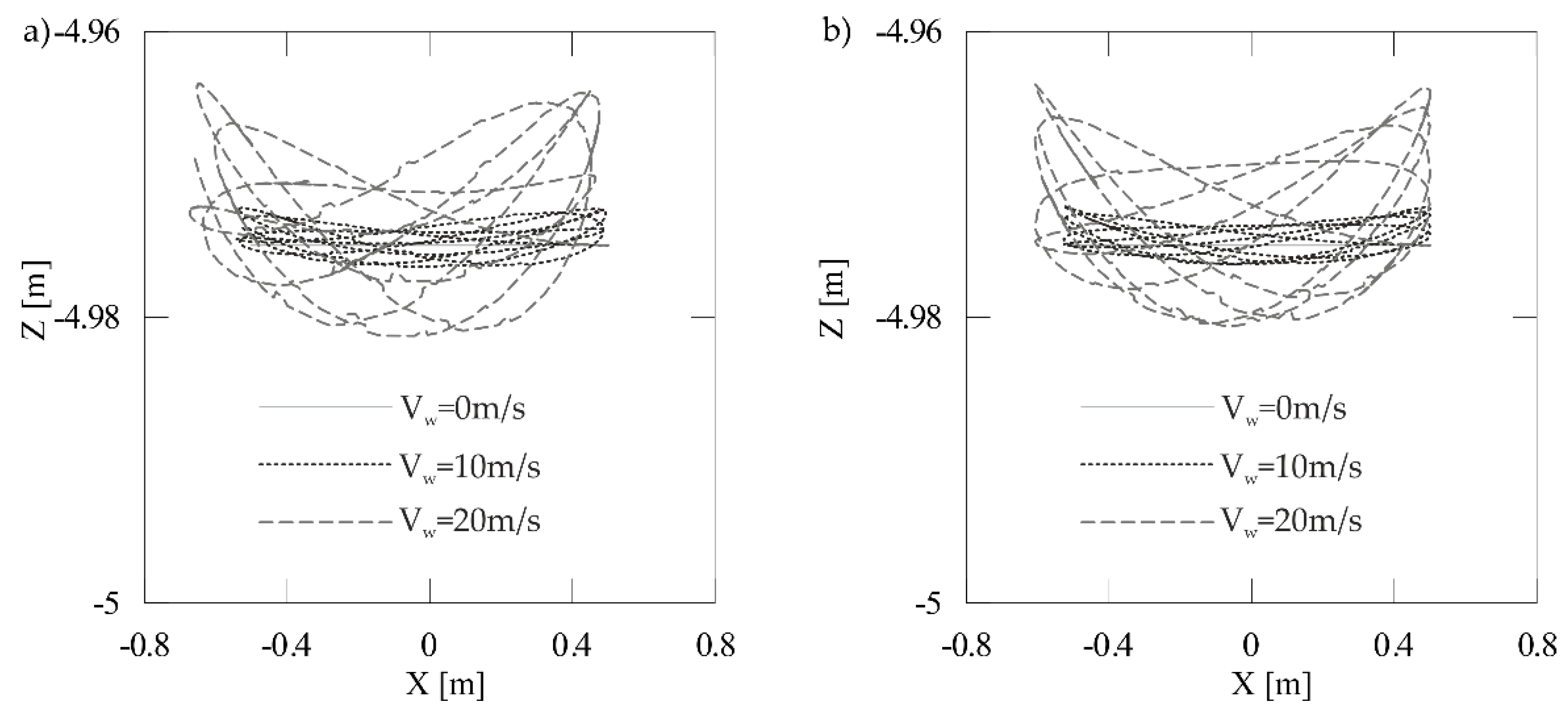
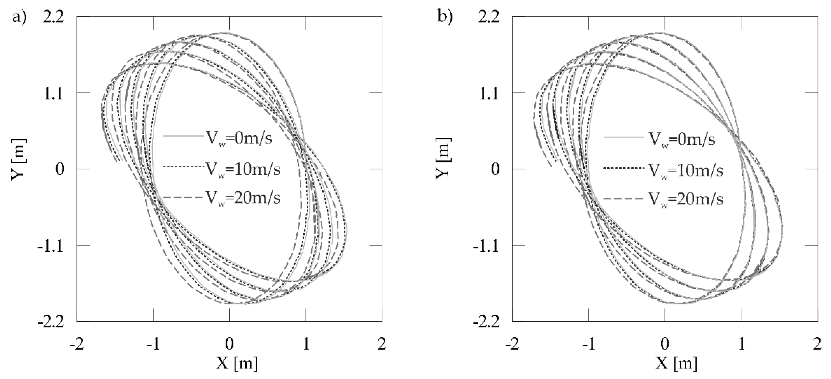
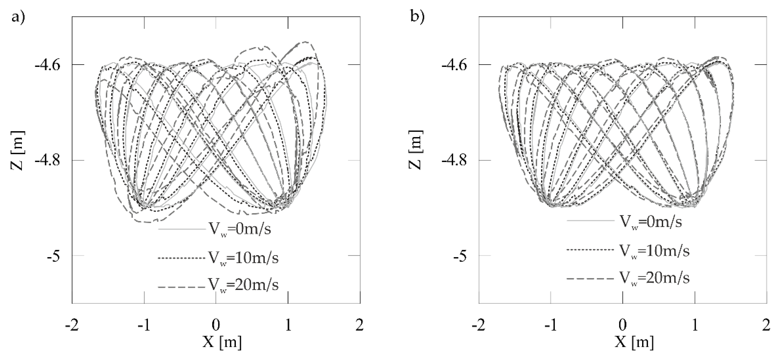
4.1. Movement of the Load as a Mathematical Pendulum

In the case where a telescopic boom remains stationary, three movement variants were considered with various initial conditions. In all cases, the load sway lasted 20 s. The influence of the variable area inclusion on which wind force had an impact on the calculations was also checked in the simulation. The sample results of numerical simulations were presented in the form of a trajectory of the load suspension—point P—and its center of mass O3, as marked in Figure 2. The values of wind power acting on the load were also determined.
The first variant pertained to load motion in only one plane, and the initial conditions were as follows:
ξ ( t ) | t = 0 = 0.5   m , ξ ˙ ( t ) | t = 0 = 0 , η ( t ) | t = 0 = 0 , η ˙ ( t ) | t = 0 = 0 , ζ ( t ) | t = 0 = 4.97494   m , ζ ˙ ( t ) | t = 0 = 0 .
Based on the obtained results (Figure 3, Figure 4, Figure 5 and Figure 6), it can be stated that in one plane motion, the parameter of the variability of surface area influenced by wind power has a negligible effect on the trajectory of analyzed points. The maximum difference in the value of wind power (Figure 7) for a given case reached 40 N for a wind velocity of 10 m/s and 170 N for 20 m/s.
In the second case, the rotational motion of the pendulum was analyzed by adopting the following initial conditions:
ξ ( t ) | t = 0 = 0.5   m , ξ ˙ ( t ) | t = 0 = 0 , η ( t ) | t = 0 = 0 , η ˙ ( t ) | t = 0 = 0.702119   m / s , ζ ( t ) | t = 0 = 4.97494   m , ζ ˙ ( t ) | t = 0 = 0 .
Based on obtained results for rotational motion (Figure 8, Figure 9, Figure 10 and Figure 11), it can be noticed that the parameter of surface area variability, on which wind power impacts, has a strong effect on the analyzed points trajectory. The difference in the value of wind power for this case reached 200 N for a wind velocity of 10 m/s and 1000 N for 20 m/s (Figure 12). Comparing wind powers as a function of time (Figure 12), similarities in trends can be noticed.
The final variant that was analyzed concerning the stationary boom depicts the spatial motion of the load:
ξ ( t ) | t = 0 = 1   m , ξ ˙ ( t ) | t = 0 = 0 , η ( t ) | t = 0 = 0 , η ˙ ( t ) | t = 0 = 2.83016 m / s , ζ ( t ) | t = 0 = 4.89898   m , ζ ˙ ( t ) | t = 0 = 0 .
Considering the results achieved with spatial motion (Figure 13, Figure 14, Figure 15 and Figure 16), the criterion of surface area variability on which wind power acted affects the trajectory of analyzed points. The different values of wind power for this variant have reached 300 N for a wind velocity of 10 m/s and 1200 N for 20 m/s. By contrasting the wind powers as a function of time (Figure 17), more significant differences in the path can be noticed than in the first variant of motion.
The presented results of numerical calculations (Figure 3, Figure 4, Figure 5, Figure 6, Figure 7, Figure 8, Figure 9, Figure 10, Figure 11, Figure 12, Figure 13, Figure 14, Figure 15, Figure 16 and Figure 17) illustrate the response of the system in the form of load motion with respect to given initial conditions in relation to the stationary telescopic boom. The obtained results allow for accuracy verification of the calculation model. The trajectories of load suspension and its center of mass were presented regarding the movement in the YOZ plane (Figure 3, Figure 4, Figure 5 and Figure 6), rotational motion (Figure 8, Figure 9, Figure 10 and Figure 11), and spatial motion of the pendulum (Figure 13, Figure 14, Figure 15 and Figure 16). The value change of wind force power is depicted in Figure 7, Figure 12, and Figure 17. By analyzing the obtained results, it is possible to observe differences between the parameter of the effective area and the fixed area. Depending on the analyzed variant, the values of wind power were different by even 1200 N, according to the considered area and wind power. More considerable differences regarding the influence of wind power in the trajectory of the load were also observed in the lifting plane rather than in the rotary plane. Based on the presented results, an effective area parameter was adopted in the subsequent numerical simulations pertaining to telescopic boom movement. Differences between trajectories depending on wind velocity were also noted. The higher the wind velocity: the greater load deflection. For the fixed surface area parameter (as opposed to the variable parameter), smaller deflections caused by wind power were observed.

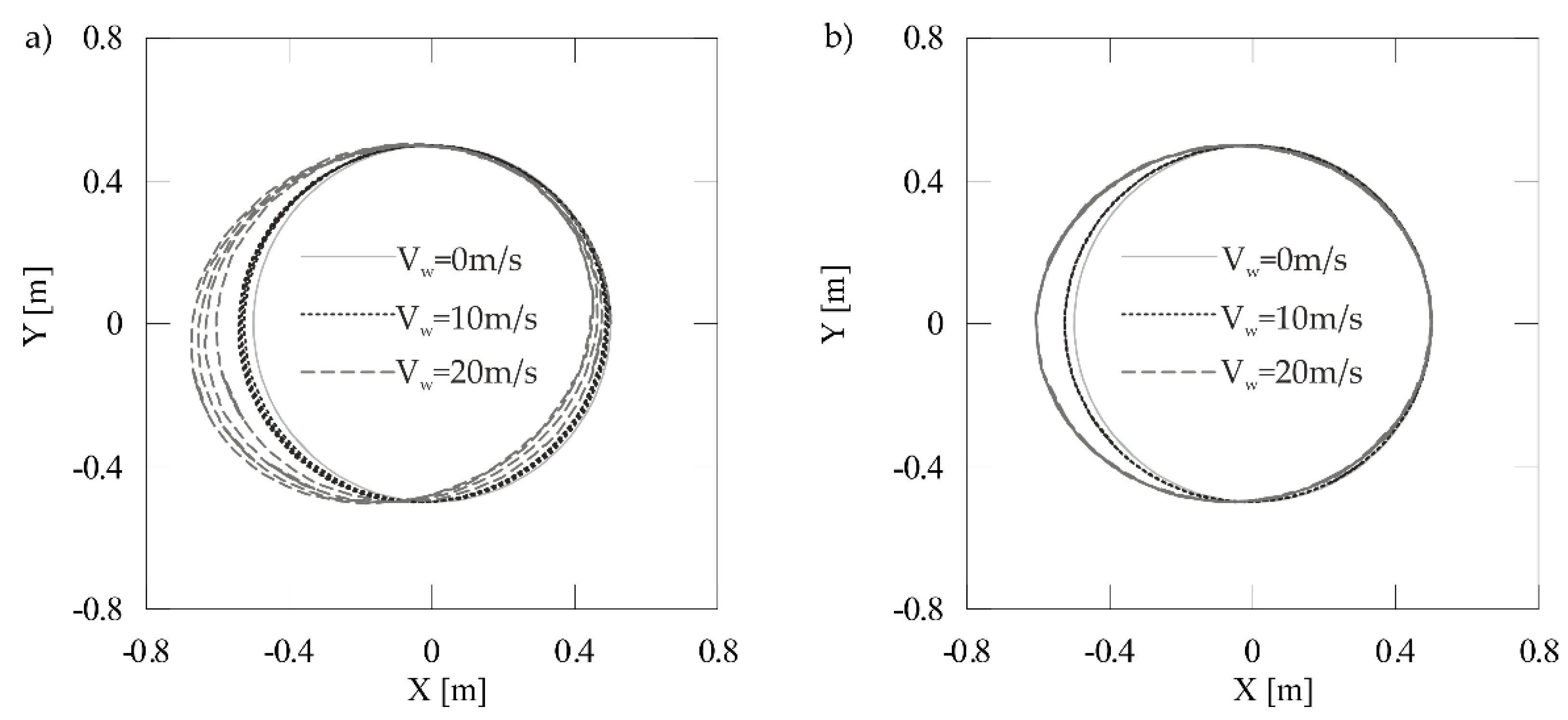
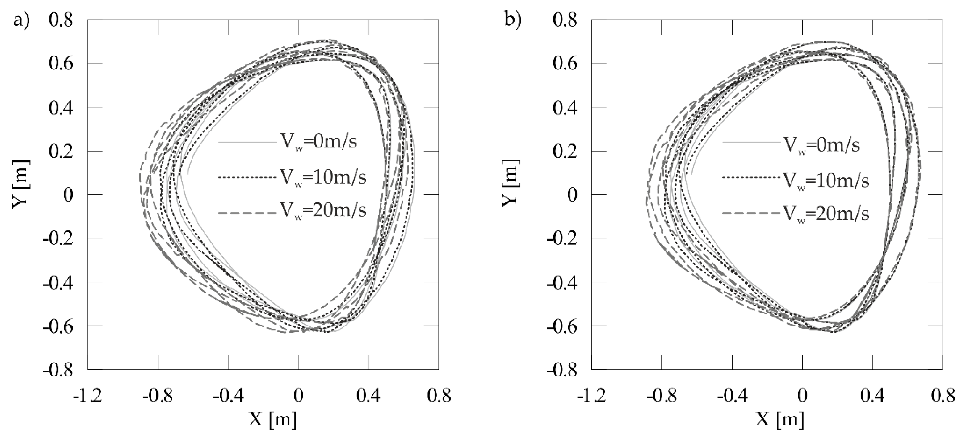
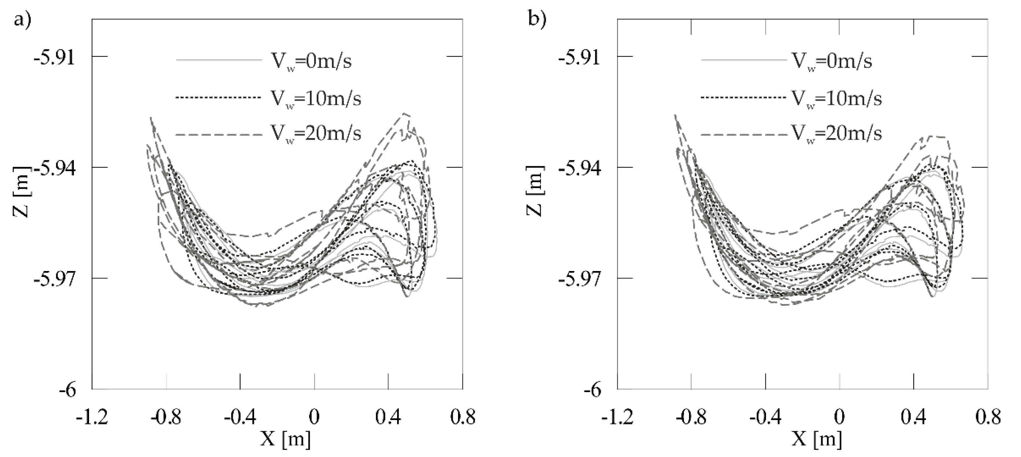
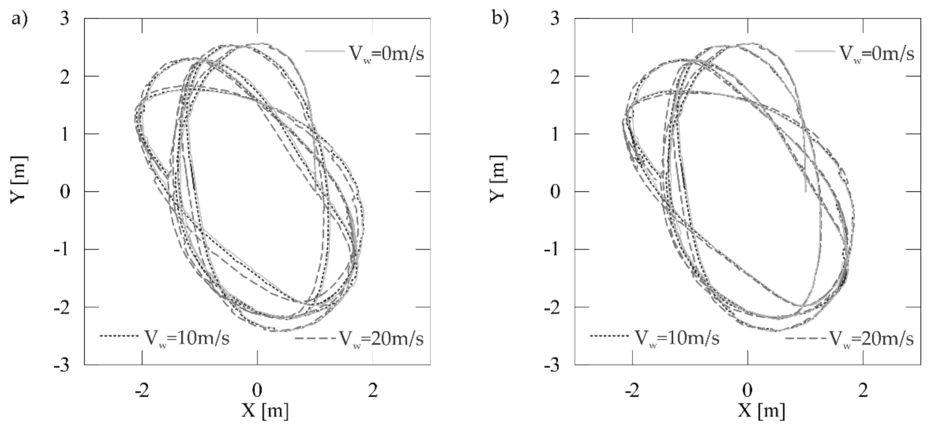
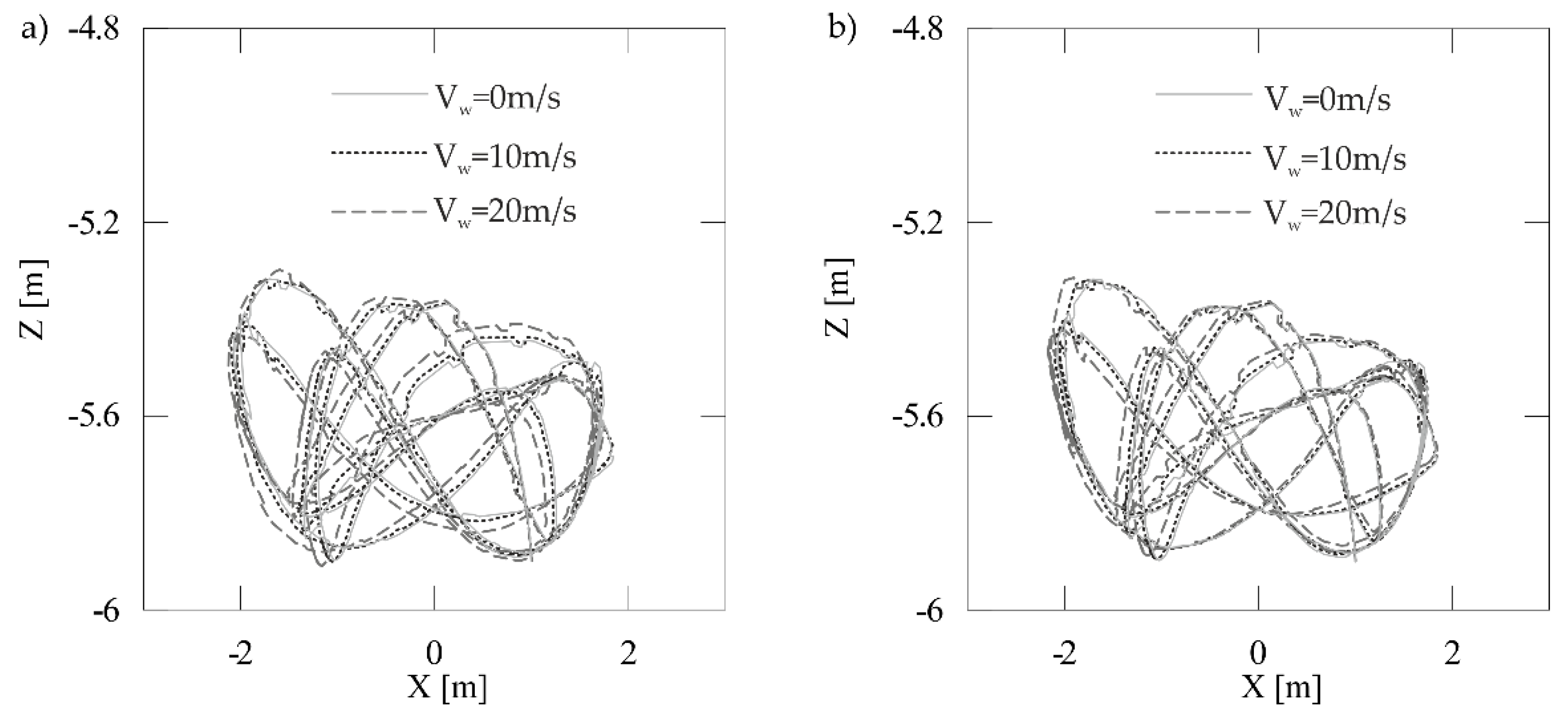
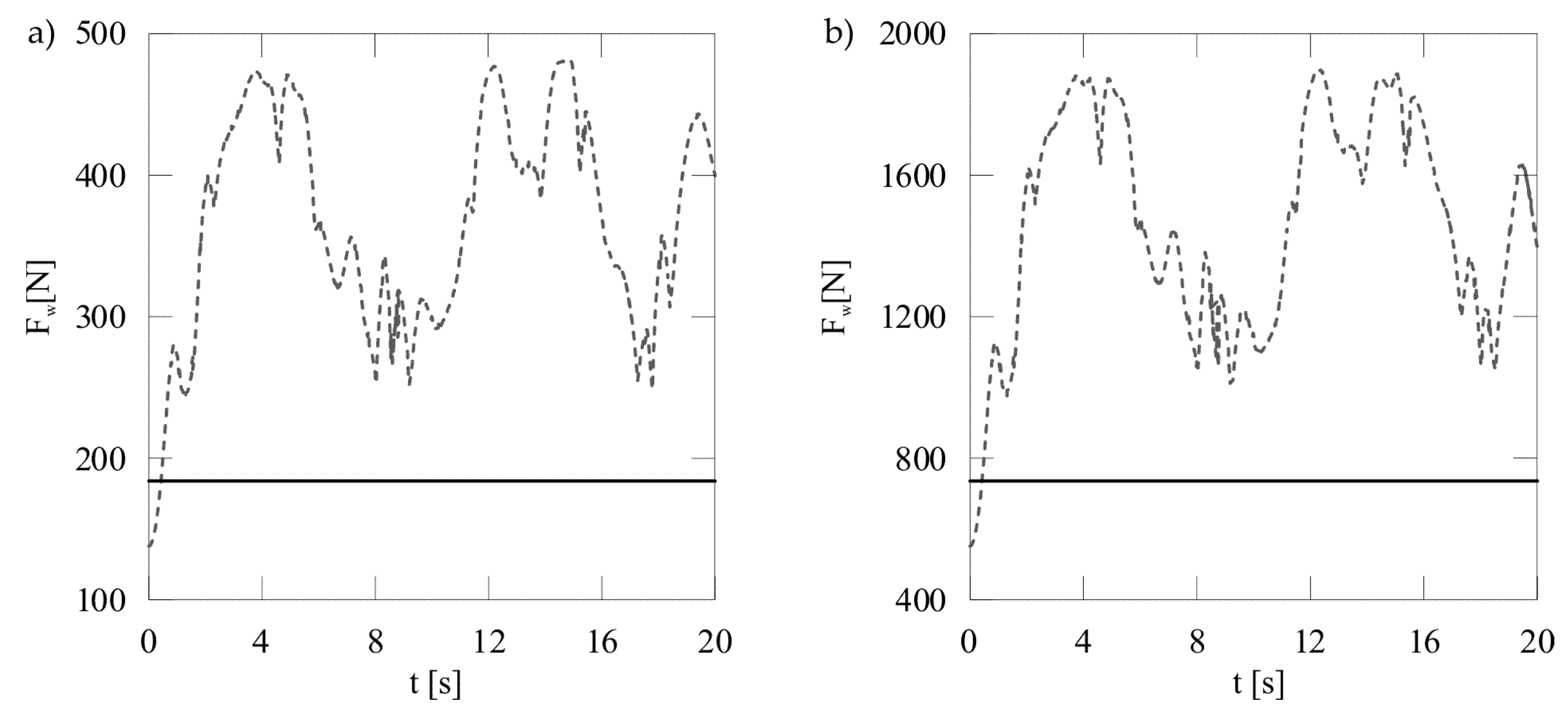
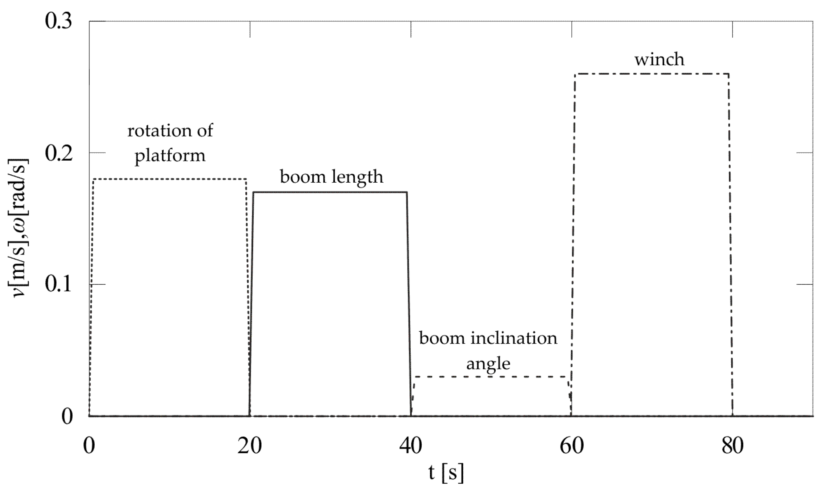
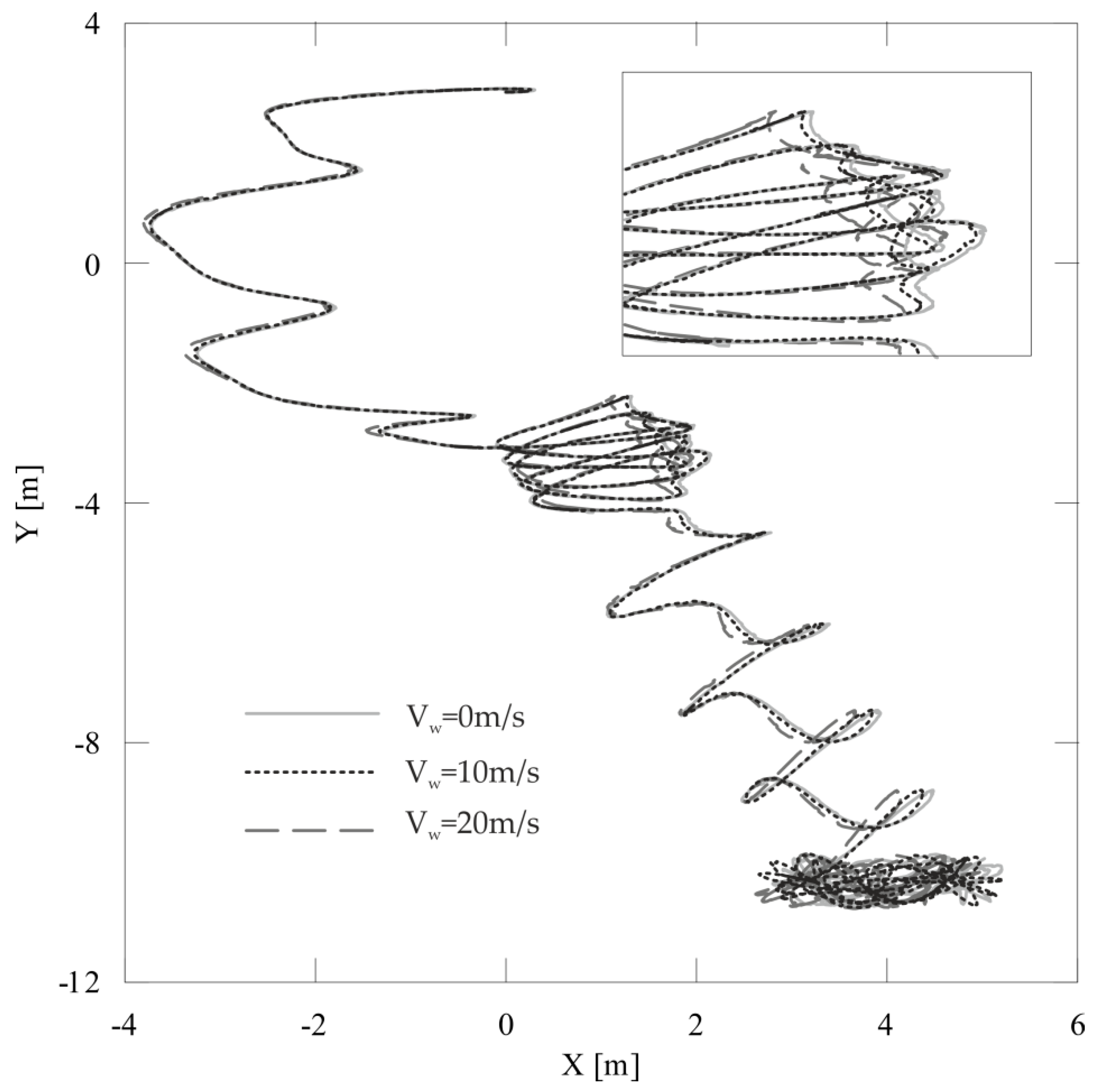
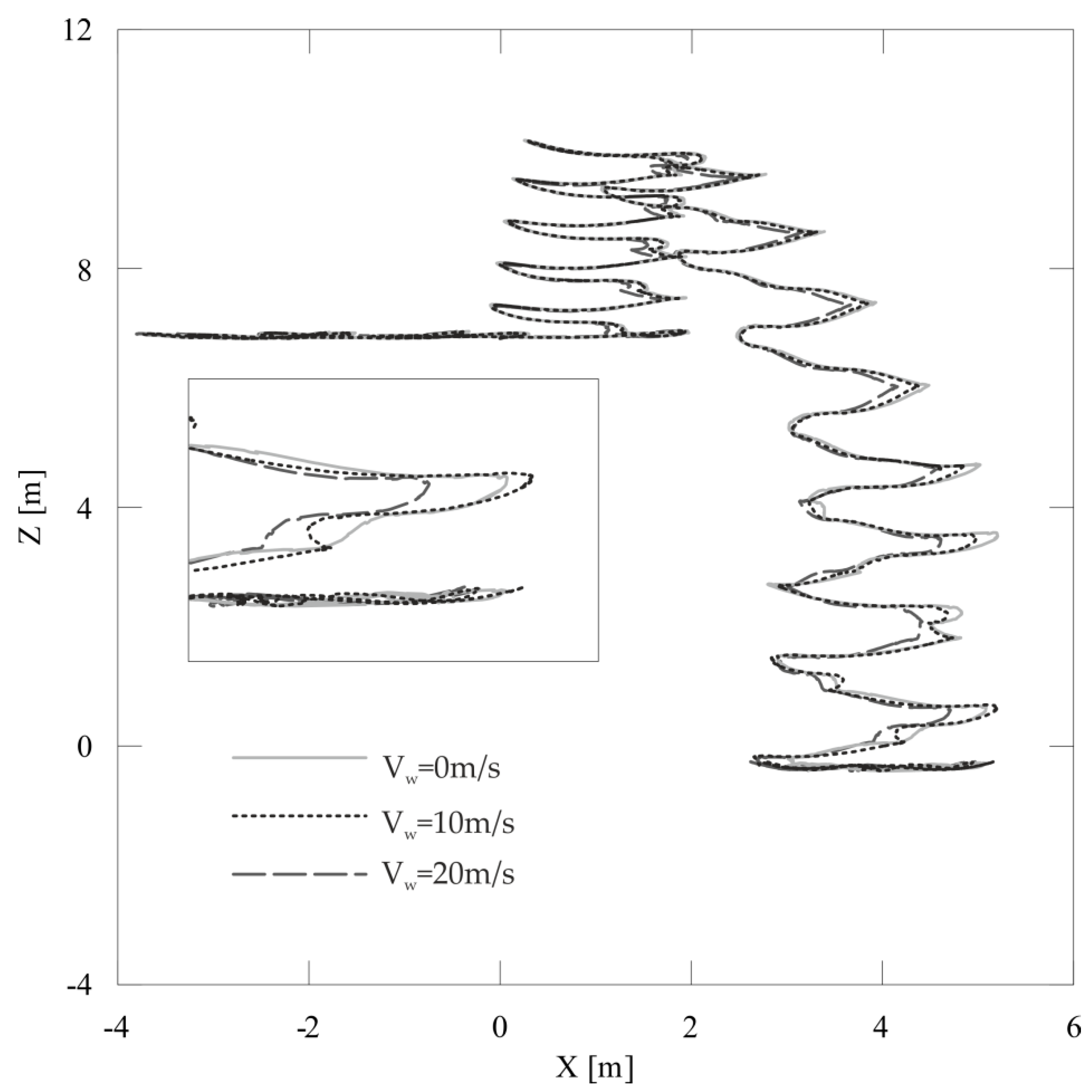
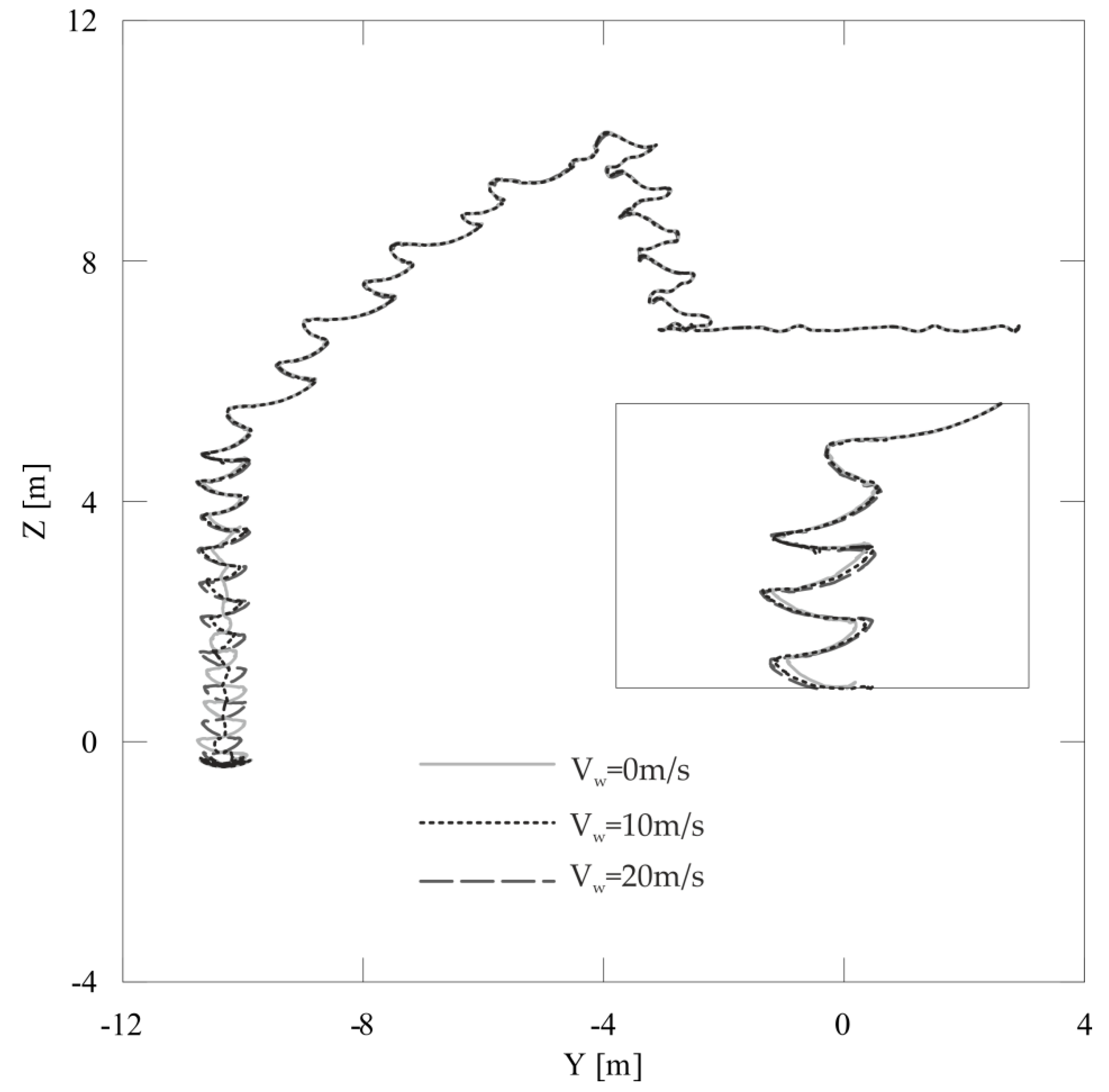
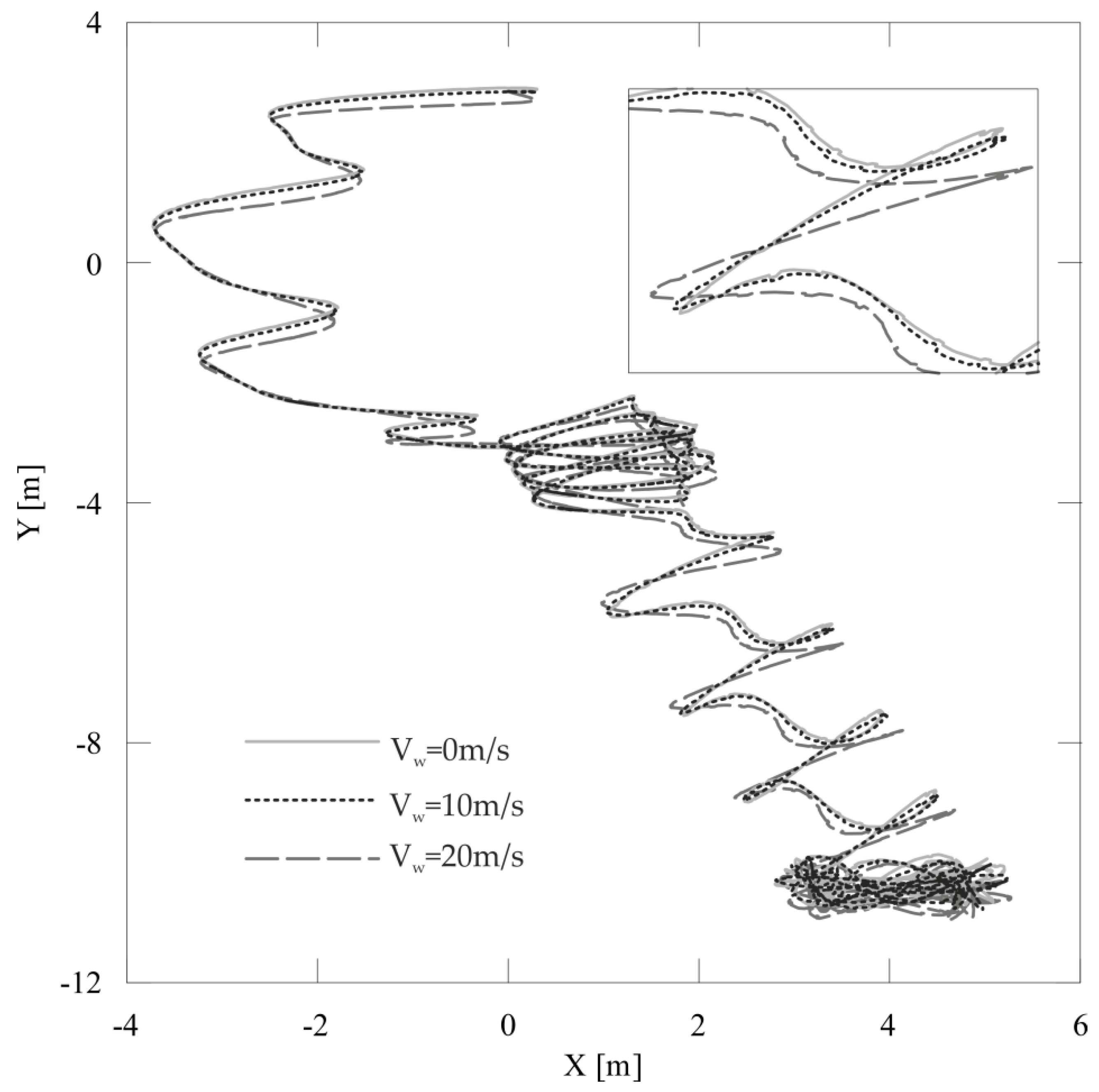
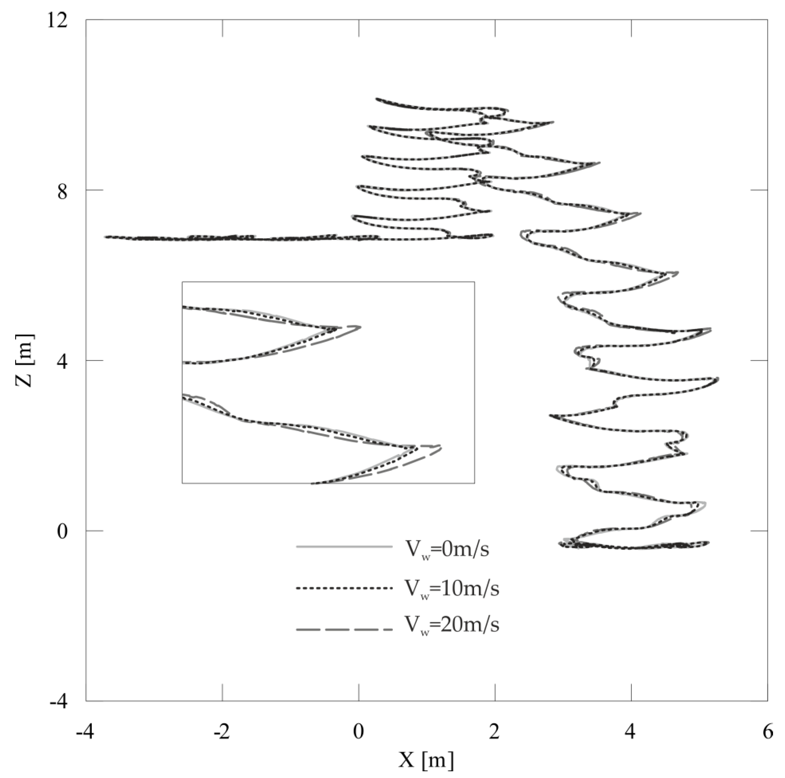
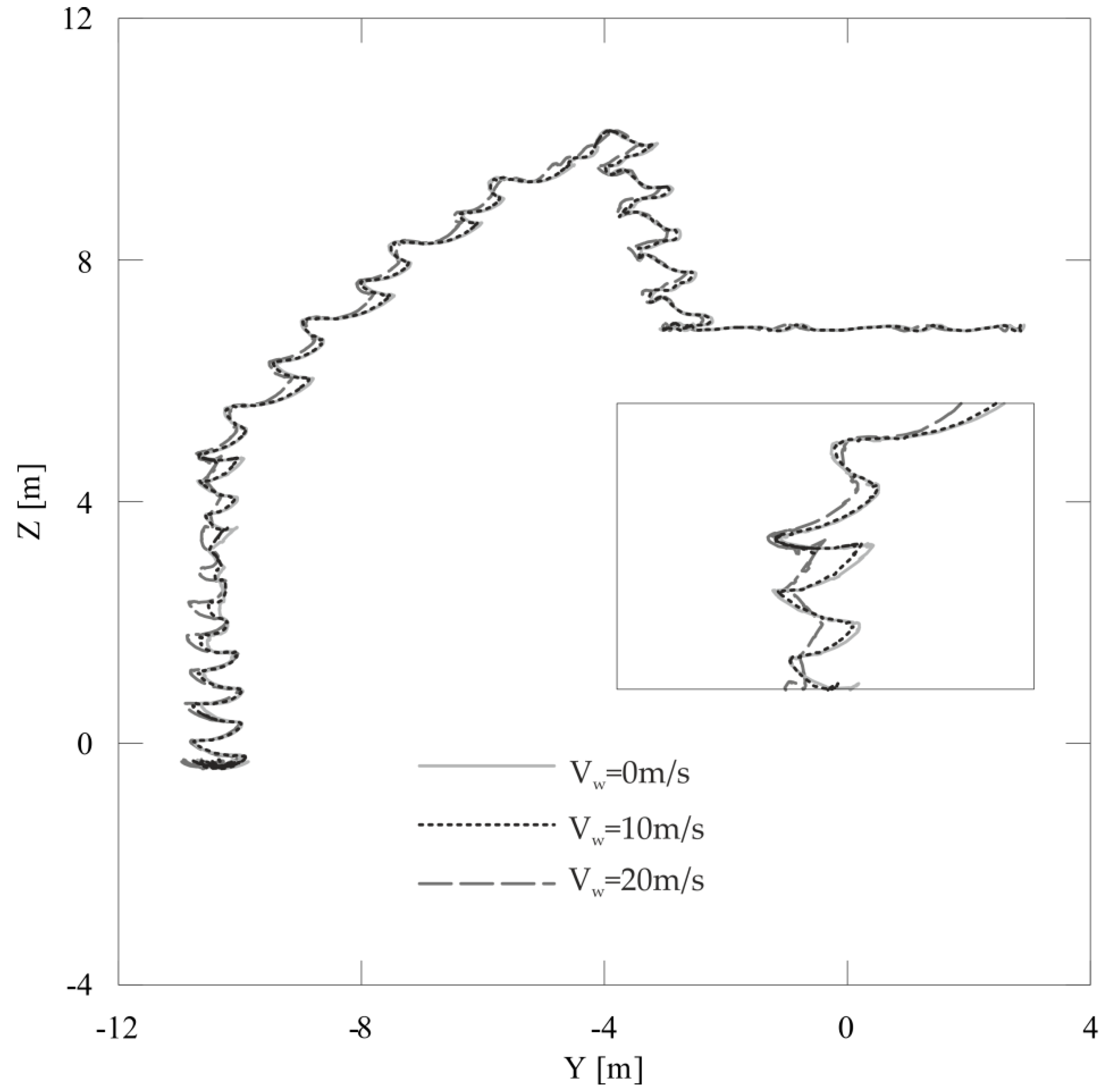
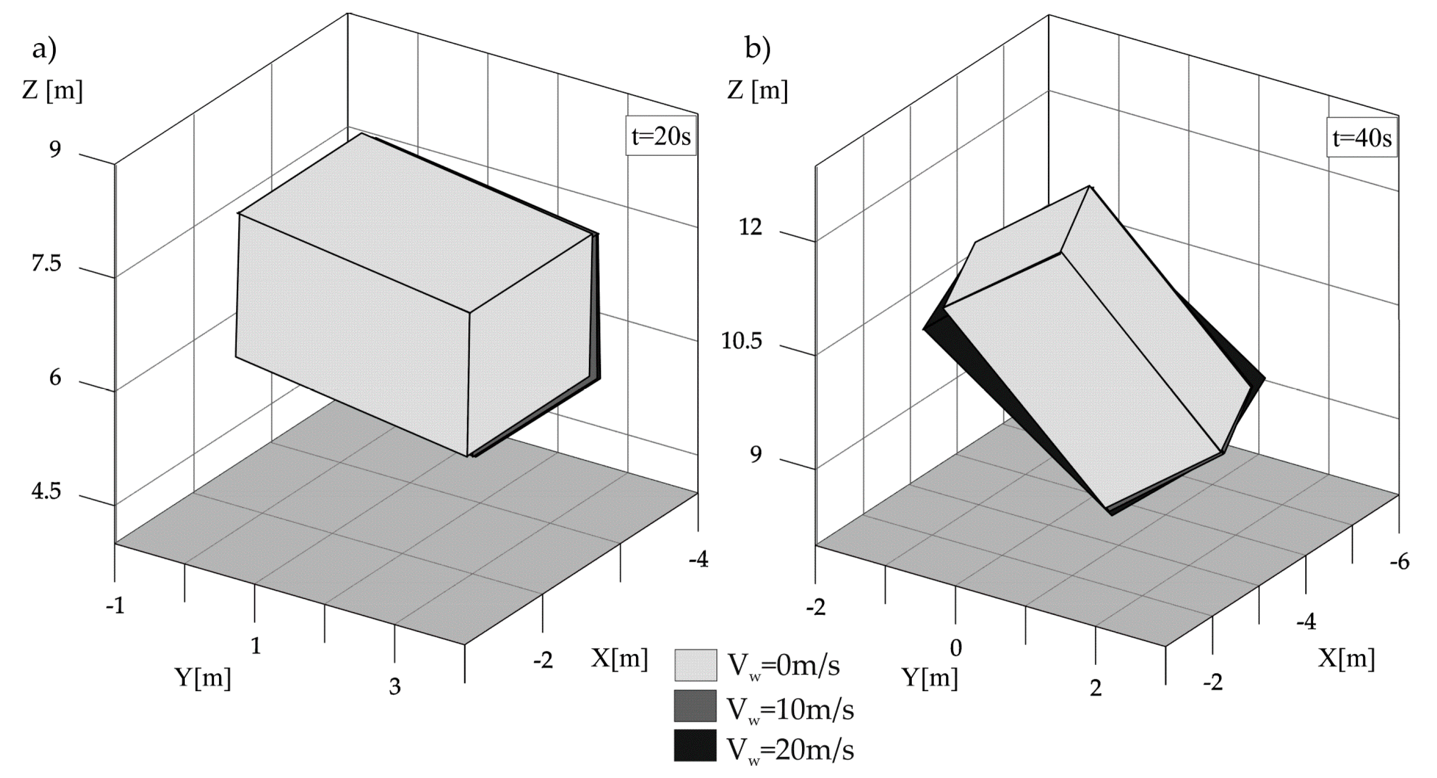
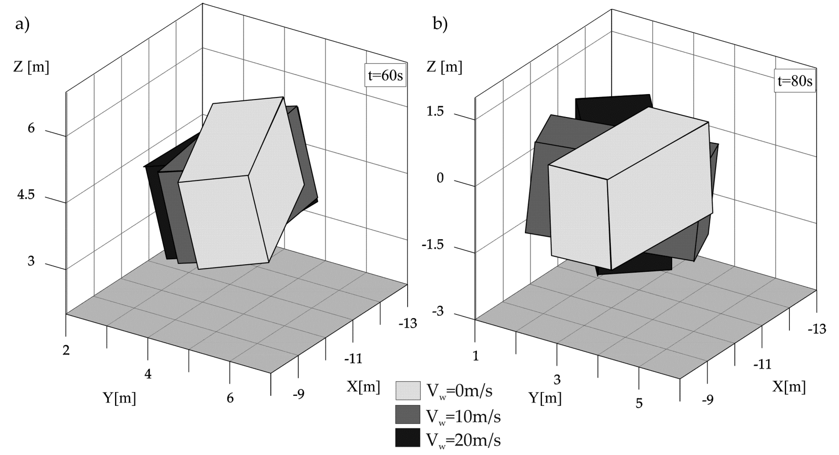
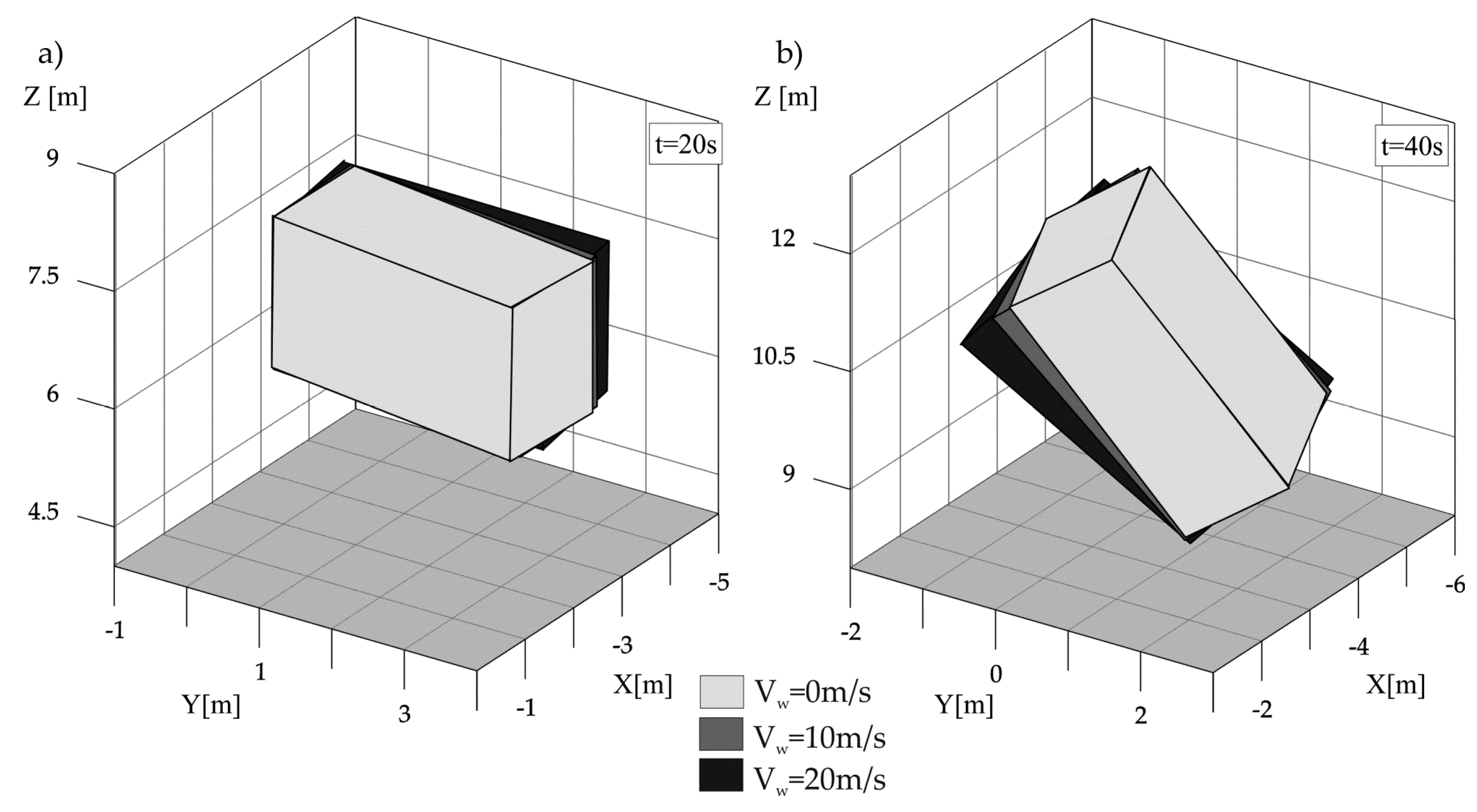
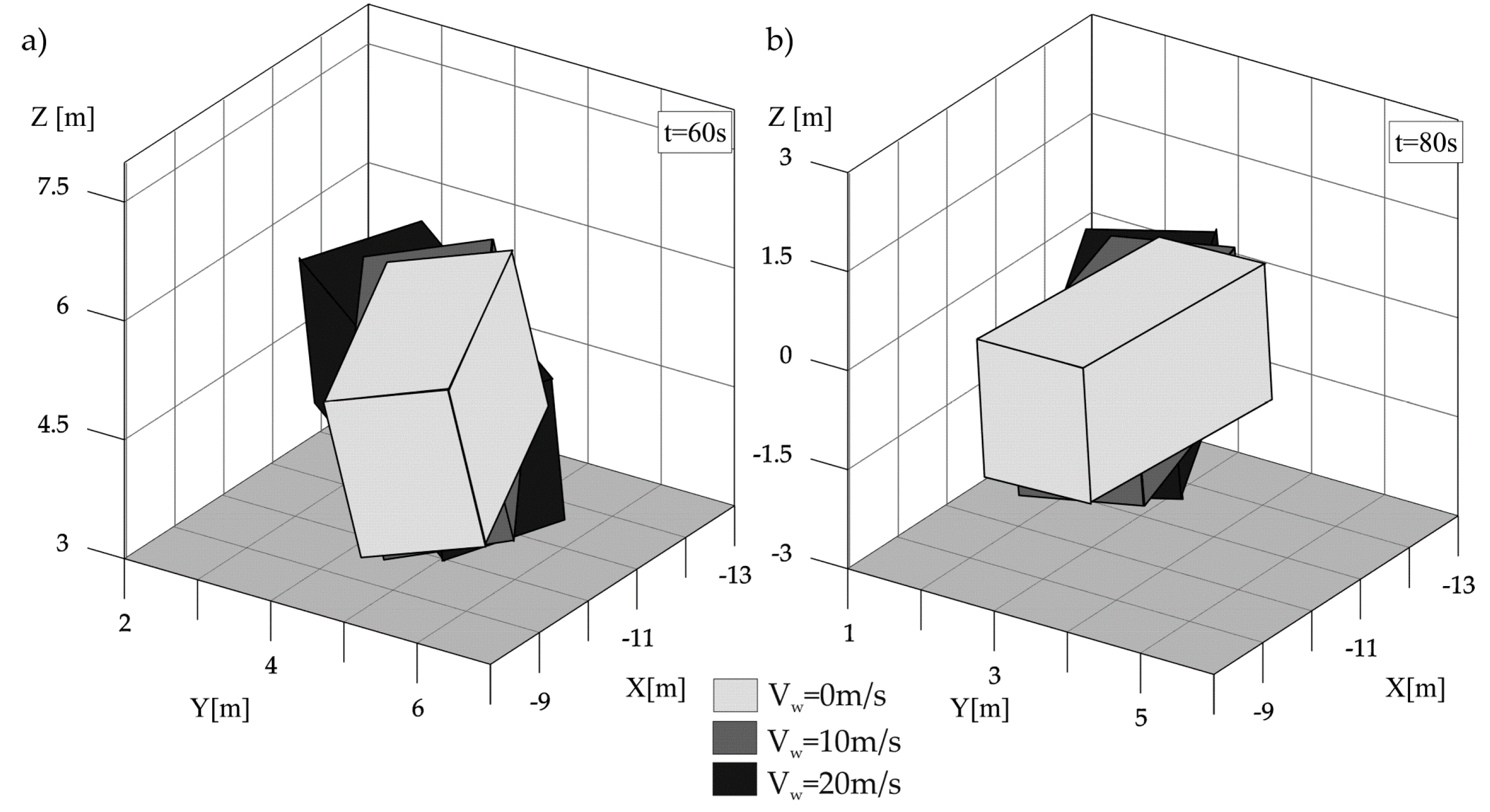
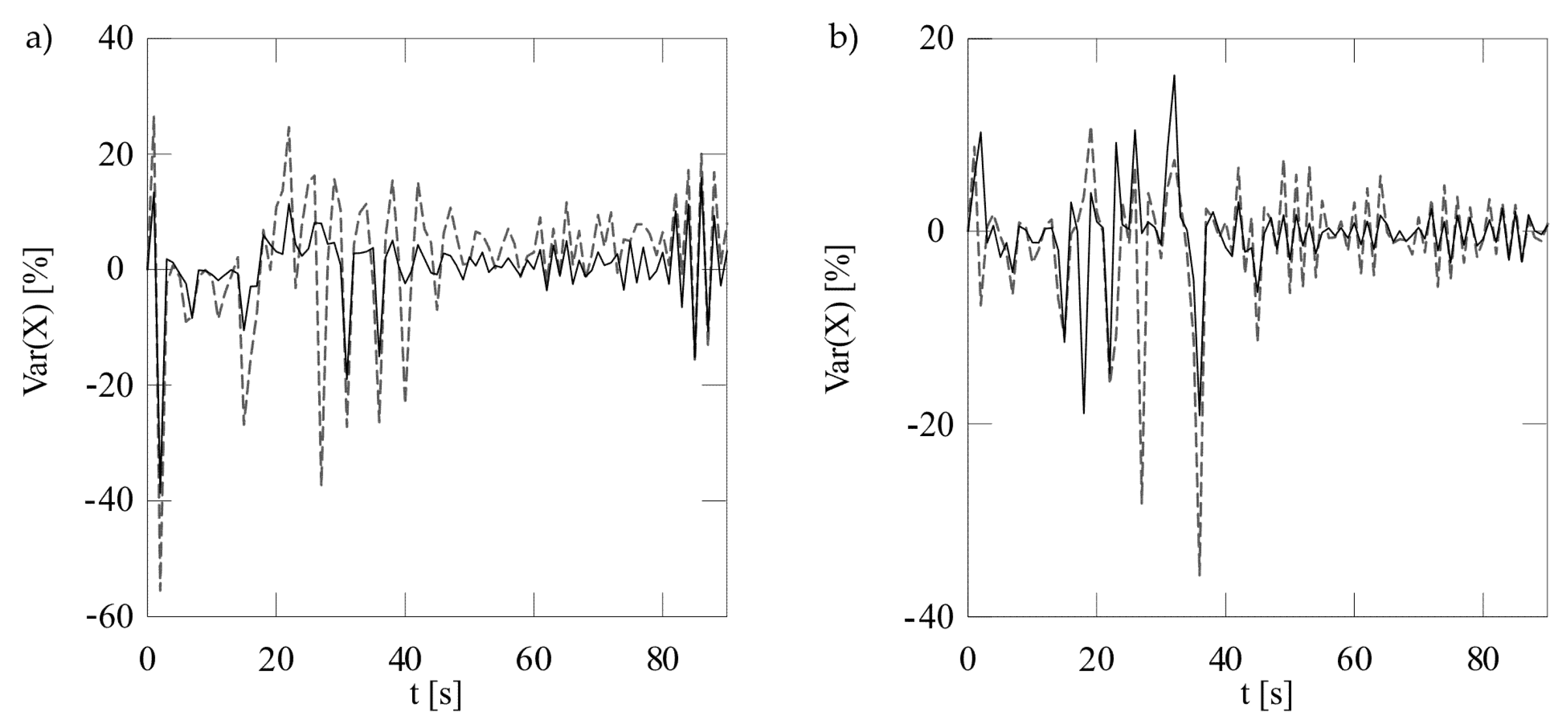
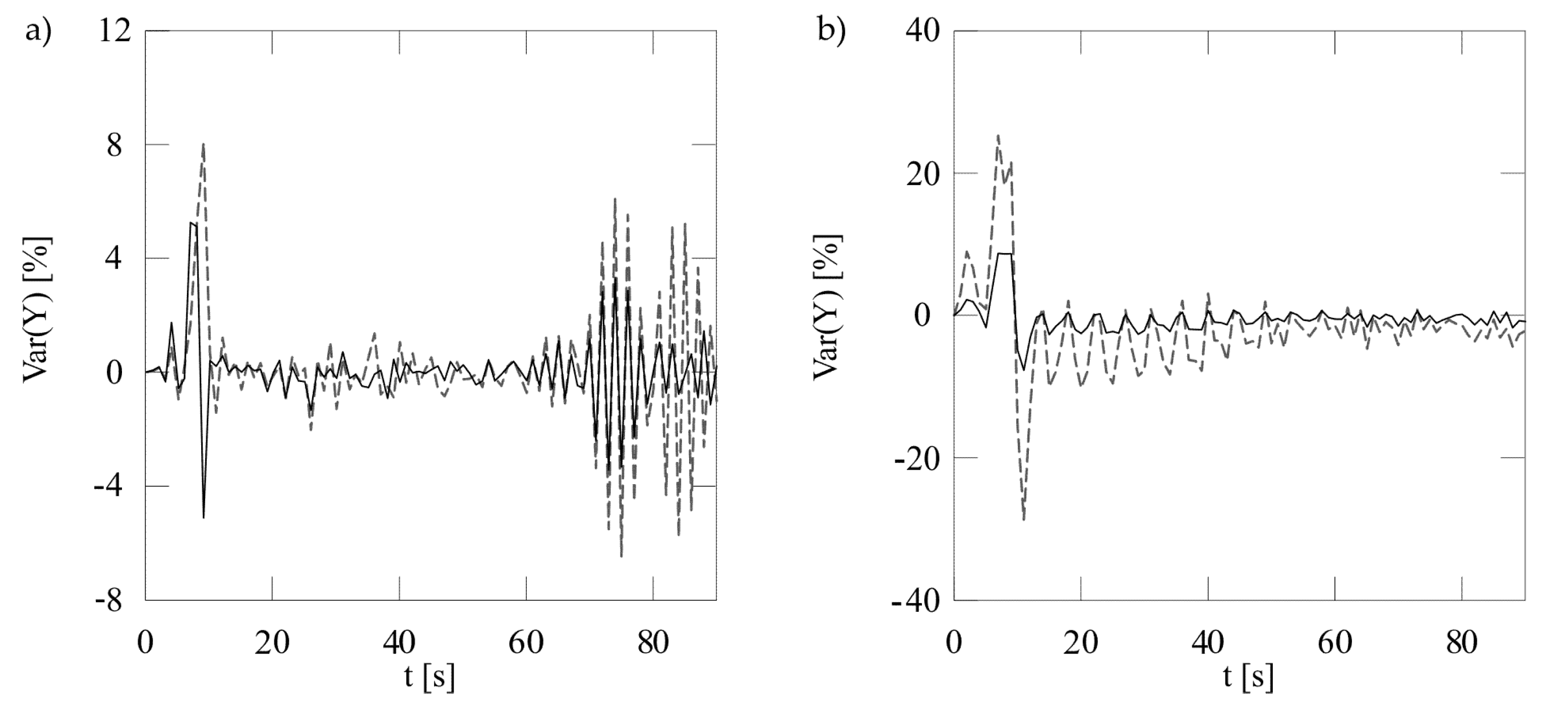
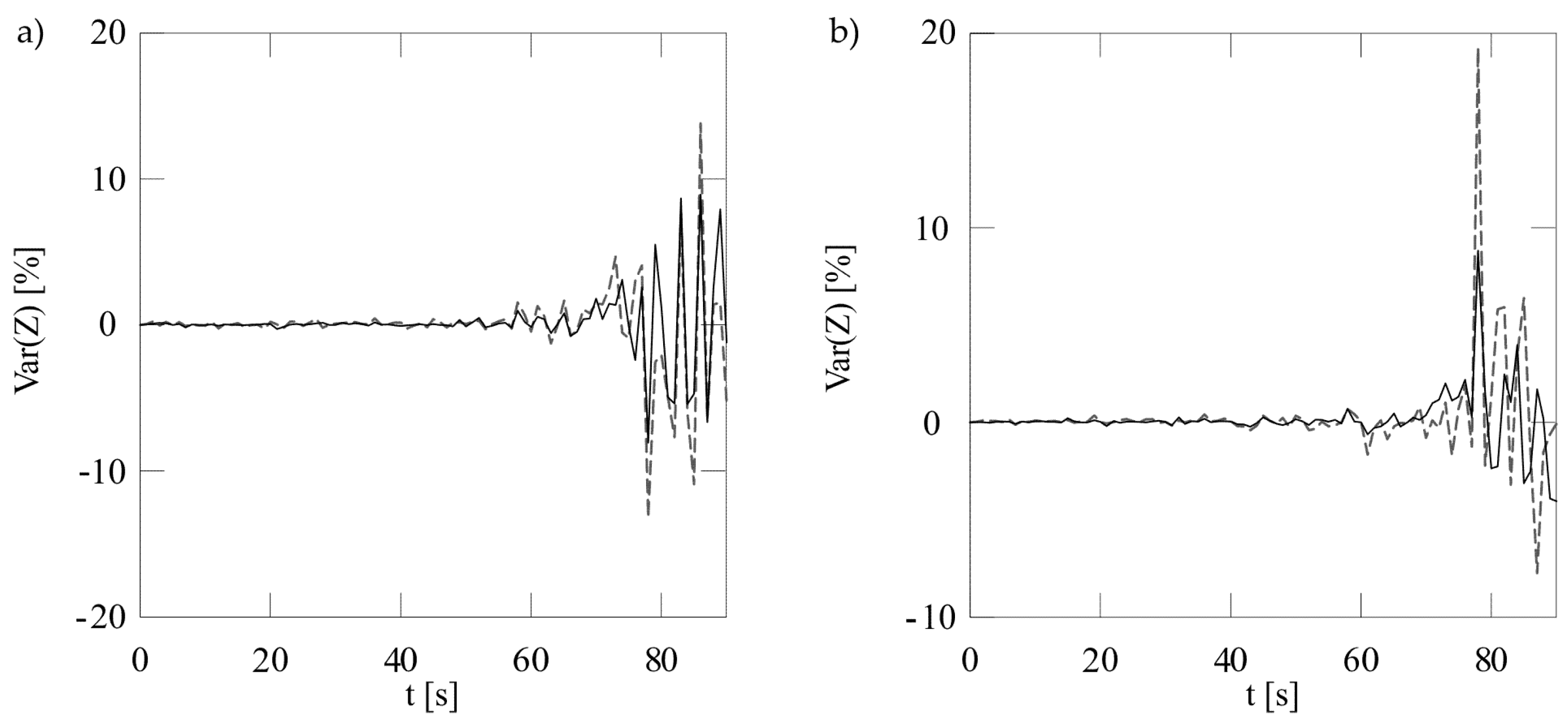
4.2. The Movement of the Load during the Working Cycle of the Truck-Crane

Example simulation studies involving telescopic boom movement were conducted with respect to two cases, differing in terms of wind power direction influence. Kinematic forces were presented in the form of trapezoidal impulses which covered start-up, steady motion, and braking movement (Figure 17). In the simulation studies, the start-up and braking movement lasted half a second. The total time of the studies covered an 80 s forced movement of the system and a 10 s free movement of the load.
In the present calculations, initial conditions were adopted where the load was hanging free, while the adopted control functions (Figure 18) are not overlapping and respectively result from:
  • the control of the crane’s platform rotation together with the telescopic boom—the motion starts at 0 s and lasts for 20 s, the maximum velocity in this motion is equal to 0.18 rad/s
  • the control of the working-stroke of the hydraulic actuator system responsible for the change of the total length of the boom—the motion starts at 20 s and lasts for 20 s, the maximum velocity is equal to 0.18 m/s
  • the control of the power stroke of the hydraulic actuator of boom change—the forcing lasts for 20 s and starts at 40 s, the maximum velocity is equal to 0.036 rad/s
  • the control of winch operation—a 20 s cable extension begins at 60 s, the maximum velocity of cable extension is 0.27 m/s
The initial conditions were adopted in the following form:
ξ ( t ) | t = 0 = 0 , ξ ˙ ( t ) | t = 0 = 0 , η ( t ) | t = 0 = 0 , η ˙ ( t ) | t = 0 = 0 , ζ ( t ) | t = 0 = 5   m , ζ ˙ ( t ) | t = 0 = 0 ,
where the value of the generalized coordinate ζ results from the initial cable’s length.
The response of the system to the adopted kinematic forcing (Figure 18) was obtained in the form of projections of the carried load’s center of mass trajectories in the rotation and lifting planes (Figure 19, Figure 20, Figure 21, Figure 22, Figure 23 and Figure 24). The vertex coordinates of the load provide a presentation of the spatial orientation of said load after the cessation of the control functions operation (Figure 25, Figure 26, Figure 27 and Figure 28).
On the basis of the results for carried load motion during the crane work cycle, the highest deflections of the load were noticed in the X axis wind direction. Observed was that the inclusion of wind power in the model causes slight differences in load trajectory. However, at some points in time, significant changes in the direction of motion were noticed. Changes in the direction of motion, in several cases, may even lead to a loss of crane stability. In the considered case, the most significant payload oscillations caused by wind power were seen in the last two control functions—boom inclination angle and winch.
During the working cycle of a truck crane, one of the most important criteria, besides the loss of stability, is correct positioning of the carried load. In Figure 25, Figure 26, Figure 27 and Figure 28, the orientation of the load in particular moments of time can be observed. When wind power has impact in the X axis direction (Figure 25 and Figure 26), the biggest differences can be noticed when winch operation ends (Figure 26b). Significant changes were also noted at the end of boom angle change motion (Figure 26a). Smaller differences in the positioning of the load for Y axis wind power direction were observed in Figure 28. The cause is the smaller effective area affected by wind force during the crane’s working cycle. However, the Y axis wind power direction, in this case, causes higher inclinations after crane platform rotation and boom length extension.
On the basis of the obtained results, it is possible to observe that the inclusion of wind-power impact in the calculation model causes differences in the trajectories of load movement path (Figure 19, Figure 20, Figure 21, Figure 22, Figure 23 and Figure 24) and in the load positioning process concerning particular moments of time (Figure 25, Figure 26, Figure 27 and Figure 28). While analyzing the crane work cycle, including the control functions (Figure 18), greater differences were noted in the load motion trajectory in the rotation plane rather than in the lifting planes.
Percentages of variation of load center mass coordinates with different directions of wind pressure are shown in Figure 29, Figure 30 and Figure 31. The most significant difference between trajectories with and without wind was noticed for X coordinate when wind power has impact according to the X axis direction (Figure 29). The maximum percentage of variation for the highest wind rate was 55%. This fact was caused by the position of the rigid body when the active surface area is the largest. There were also larger differences related to the direction of the wind force (Figure 29 and Figure 30). When the wind acts in the direction of the Y axis, significant differences were observed for Y coordinate (Figure 30). The maximum percentage of variation in this case was 29%, for a wind speed equal to 20 m/s. The biggest deviations from the trajectory for the Z coordinate were observed for load free motion after the kinematic forcing ceased to operate (Figure 31).

5. Conclusions

The paper presents an analysis of load movement carried by means of a mobile crane with the inclusion of wind power influence impact. The mathematical model of the analyzed system, which was developed based on a real object, was divided into a kinematic and dynamic part. In the kinematic part, motion parameters were determined. In the dynamic section, the influence of motion parameters on the dynamics of the load was analyzed.
The motion of the load, treated as a nondeformable static body, was presented as a combination of translational motion relative to origin in the global coordinate system and rotational motion relative to the load’s center of mass. Orientation and deflections of the analyzed load were determined using Bryant angles. The rectangular coordinate systems have been adopted in a way in which the relative motions of individual systems are translational motion. The force of wind impact was determined using the formula for drag resistance. A system of six ordinary differential equations of the 2nd degree was obtained which, taking into account the initial conditions, constituted a full description of the initial problem of load motion. The parameter of the variability of surface area on which wind power had influence was also presented.
The results of numerical simulations were presented for two cases of system motion– mathematical pendulum (fixed telescopic boom—Ω point) and working cycle of rotating crane.
The first part of the work pertains to the case where the telescopic boom remained stationary, and the load was treated as a mathematical pendulum. Three variants of movement were analyzed: in the YOZ plane, rotational motion, and spatial motion, which enabled validation of the computational model. Three values of wind velocity were studied in accordance with the guidelines from Poland’s standards regarding safety and mobile crane operation. The effective area influence of wind power on load motion was also considered. The results were presented in the form of trajectory projections of the suspension point and the center of load mass in the lifting and rotation planes.
The second part of the paper includes an analysis of the wind impact influence during a crane’s working cycle. The model includes the parameter of the load’s effective area on which wind power had impact. Two cases were considered that varied in terms of wind impact direction. The results were presented in the form of trajectory projections of the center of mass and figures showing load orientation in space concerning particular moments of time. During the determination of load orientation in relation to the same kinematic forcing, greater inclinations caused by wind-force impact acting in accordance with the direction of the X axis were found.
On the basis of the conducted simulations, it was possible to observe that wind force has an influence on the trajectory and the inclinations of the carried load and that it should be considered during studies on load dynamics, system stability, or final positioning.

Author Contributions

Conceptualization, D.C. and R.G.; methodology, P.K.; software, D.C. and P.K.; validation, D.C., P.K. and R.G.; formal analysis, P.K; writing—original draft preparation, P.K. and D.C.; writing—review and editing, R.G. and P.K.; supervision, D.C.; Funding Acquisition, R.G.

Funding

This research was partially funded by Poland’s Ministry of Science and Higher Education, grant number 944/P-DUN/2019.

Acknowledgments

The study has been carried out within statutory research of the Institute of Mechanics and Machine Design Fundamentals of Czestochowa University of Technology.

Conflicts of Interest

The authors declare no conflict of interest.

References

  1. Posiadała, B. Influence of crane support system on motion of the lifted load. Mech. Mach. Theory 1997, 32, 9–20. [Google Scholar] [CrossRef]
  2. Mijailović, R. Modelling the dynamic behavior of the truck-crane. Transport 2011, 26, 410–417. [Google Scholar] [CrossRef]
  3. Posiadala, B.; Warys, P.; Cekus, D.; Tomala, M. The Dynamics Of The Forest Crane During The Load Carrying. Int. J. Struct. Stab. Dyn. 2013, 13. [Google Scholar] [CrossRef]
  4. Kacalak, W.; Budniak, Z.; Majewski, M. Stability Assessment as a Criterion of Stabilization of the Movement Trajectory of Mobile Crane Working Elements. Int. J. Appl. Mech. Eng. 2018, 23, 65–77. [Google Scholar] [CrossRef] [Green Version]
  5. Romanello, G. Stability analysis of mobile cranes and determination of outriggers loading. J. Eng. Des. Technol. 2018, 16, 938–958. [Google Scholar] [CrossRef]
  6. Kłosiński, J.; Janusz, J. Control of Operational Motions of a Mobile Crane under a Threat of Loss of Stability. SSP 2008, 144, 77–82. [Google Scholar] [CrossRef]
  7. Wu, J.; Guzzomi, A.L.; Hodkiewicz, M. Static stability analysis of non-slewing articulated mobile cranes. Aust. J. Mech. Eng. 2014, 12, 60–76. [Google Scholar] [CrossRef]
  8. Sochacki, W. The dynamic stability of a laboratory model of a truck crane. Thin-Walled Struct. 2007, 45, 927–930. [Google Scholar] [CrossRef]
  9. Tran, Q.H.; Huh, J.; Nguyen, V.B.; Kang, C.; Ahn, J.H.; Park, I.J. Sensitivity analysis for ship-to-shore container crane design. Appl. Sci. 2018, 8, 1667. [Google Scholar] [CrossRef]
  10. Arena, A.; Casalotti, A.; Lacarbonara, W.; Cartmell, M.P. Dynamics of container cranes: Three-dimensional modeling, full-scale experiments, and identification. Int. J. Mech. Sci. 2015, 93, 8–21. [Google Scholar] [CrossRef]
  11. Lee, S.-J.; Kang, J.-H. Wind load on a container crane located in atmospheric boundary layers. J. Wind Eng. Ind. Aerodyn. 2008, 96, 193–208. [Google Scholar] [CrossRef]
  12. Cekus, D.; Gnatowska, R.; Kwiatoń, P. Influence of wind on the movement of the load. J. Phys. Conf. Ser. 2018, 1101, 012005. [Google Scholar] [CrossRef]
  13. Miadlicki, K.; Pajor, M.; Sakow, M. Loader crane working area monitoring system based on LIDAR scanner. In Advances in Manufacturing; Springer: Berlin/Heidelberg, Germany, 2018; pp. 465–474. [Google Scholar]
  14. Taghaddos, H.; Hermann, U.; Abbasi, A. Automated Crane Planning and Optimization for modular construction. Autom. Constr. 2018, 95, 219–232. [Google Scholar] [CrossRef]
  15. Pan, Z.; Guo, H.; Li, Y. Automated Method for Optimizing Feasible Locations of Mobile Cranes Based on 3D Visualization. Procedia Eng. 2017, 196, 36–44. [Google Scholar] [CrossRef]
  16. Cekus, D.; Kwiatoń, P. Analysis of the motion of the load carried by a laboratory mobile crane. In Proceedings of the 24th International Conference Engineering Mechanics 2018, Svratka, Czech Republic, 14–17 May 2018; pp. 137–140. [Google Scholar]
  17. Trabka, A. Influence of flexibilities of cranes structural components on load trajectory. J. Mech. Sci. Technol. 2016, 30, 1–14. [Google Scholar] [CrossRef]
  18. Fujioka, D.; Rauch, A.; Singhose, W. Tip-Over Stability Analysis of Mobile Boom Cranes with Double-Pendulum Payloads. In Proceedings of the American Control Conference 2009, St. Louis, MO, USA, 10–12 June 2009; pp. 3136–3141. [Google Scholar]
  19. Al-Humaidi, H.M.; Hadipriono Tan, F. Mobile crane safe operation approach to prevent electrocution using fuzzy-set logic models. Adv. Eng. Softw. 2009, 40, 686–696. [Google Scholar] [CrossRef]
  20. Posiadała, B.; Skalmierski, B.; Tomski, L. Motion of the lifted load brought by a kinematic forcing of the crane telescopic boom. Mech. Mach. Theory 1990, 25, 547–556. [Google Scholar] [CrossRef]
  21. Jaskot, A.; Posiadała, B.; Śpiewak, S. Dynamics modelling of the four-wheeled mobile platform. Mech. Res. Commun. 2017, 83, 58–64. [Google Scholar] [CrossRef]
  22. Baker, C.J. Ground vehicles in high cross winds part II: Unsteady aerodynamic forces. J. Fluids Struct. 1991, 5, 91–111. [Google Scholar] [CrossRef]
  23. Liao, C.; Shi, K.; Zhao, X. Predicting the Extreme Loads in Power Production of Large Wind Turbines Using an Improved PSO Algorithm. Appl. Sci. 2019, 9, 521. [Google Scholar] [CrossRef]
  24. Ahmed, W.K. Advantages and Disadvantages of Using MATLAB/ode45 for Solving Differential Equations in Engineering Applications. Int. J. Eng. 2013, 7, 25–31. [Google Scholar]
  25. Cekus, D.; Posiadała, B.; Warys, P. Integration of modeling in Solidworks and Matlab/Simulink environments. Arch. Mech. Eng. 2014, 61, 57–74. [Google Scholar] [CrossRef]
  26. Weerasuriya, A.U.; Tse, K.T.; Zhang, X.; Kwok, K.C.S. Equivalent wind incidence angle method: A new technique to integrate the effects of twisted wind flows to AVA. Build. Environ. 2018, 139, 46–57. [Google Scholar] [CrossRef]
  27. Hazewinkel, M. Encyclopaedia of Mathematics, 1st ed.; Kluwer Academic Publishers: Dordrecht, The Netherlands, 1995. [Google Scholar]
Figure 1. Model of the system: truck crane—carried load.
Applsci 09 03842 g001
Figure 2. Forces acting on the load during the work cycle.
Applsci 09 03842 g002
Figure 3. Projection of the trajectory of the carried load’s suspension point on the rotation plane for (a) the variable effective area and (b) fixed effective area.
Applsci 09 03842 g003
Figure 4. Projection of the trajectory of the carried load’s suspension point on one of the lifting planes for (a) the variable effective area and (b) fixed effective area.
Applsci 09 03842 g004
Figure 5. Projection of the trajectory of the carried load’s suspension point on the rotation plane for (a) the variable effective area and (b) fixed effective area.
Applsci 09 03842 g005
Figure 6. Projection of the trajectory of the carried load’s suspension point on one of the lifting planes for (a) the variable effective area and (b) fixed effective area.
Applsci 09 03842 g006
Figure 7. Value of the wind impact force with respect to wind velocity equal to (a) 10 m/s and (b) 20 m/s (continuous line—fixed area, dotted line—variable area).
Applsci 09 03842 g007
Figure 8. Projection of the trajectory of the carried load’s suspension point on the rotation plane for (a) the variable effective area and (b) fixed effective area.
Applsci 09 03842 g008
Figure 9. Projection of the trajectory of the carried load’s suspension point on one of the lifting planes for (a) the variable effective area and (b) fixed effective area.
Applsci 09 03842 g009
Figure 10. Projection of the trajectory of the carried load’s suspension point on the rotation plane for (a) the variable effective area and (b) fixed effective area.
Applsci 09 03842 g010
Figure 11. Projection of the trajectory of the carried load’s suspension point on one of the lifting planes for (a) the variable effective area and (b) fixed effective area.
Applsci 09 03842 g011
Figure 12. Value of the wind impact force with respect to wind velocity equal to (a) 10 m/s and (b) 20 m/s (continuous line—fixed area, dotted line—variable area).
Applsci 09 03842 g012
Figure 13. Projection of the trajectory of the carried load’s suspension point on the rotation plane for (a) the variable effective area and (b) fixed effective area.
Applsci 09 03842 g013
Figure 14. Projection of the trajectory of the carried load’s suspension point on one of the lifting planes for (a) the variable effective area and (b) fixed effective area.
Applsci 09 03842 g014
Figure 15. Projection of the trajectory of the carried load’s suspension point on the rotation plane for (a) the variable effective area and (b) fixed effective area.
Applsci 09 03842 g015
Figure 16. Projection of the trajectory of the carried load’s suspension point on one of the lifting planes for (a) the variable effective area and (b) fixed effective area.
Applsci 09 03842 g016
Figure 17. Value of the wind impact force with respect to wind velocity equal to (a) 10 m/s and (b) 20 m/s (continuous line—fixed area, dotted line—variable area).
Applsci 09 03842 g017
Figure 18. Control functions (crane actions).
Applsci 09 03842 g018
Figure 19. Trajectory projections of the carried load’s center of mass in the rotation plane (wind power having impact according to the direction of the X axis).
Applsci 09 03842 g019
Figure 20. Trajectory projections of the carried load’s center of mass in one of the lifting planes (wind power having impact according to the direction of the X axis).
Applsci 09 03842 g020
Figure 21. Trajectory projections of the carried load’s center of mass in one of the lifting planes (wind power having impact according to the direction of the X axis).
Applsci 09 03842 g021
Figure 22. Trajectory projections of the carried load’s center of mass in the rotation plane (wind power having impact according to the direction of the Y axis).
Applsci 09 03842 g022
Figure 23. Trajectory projections of the carried load’s center of mass in one of the lifting planes (wind power having impact according to the direction of the Y axis).
Applsci 09 03842 g023
Figure 24. Trajectory projections of the carried load’s center of mass in one of the lifting planes (wind power having impact according to the direction of the Y axis).
Applsci 09 03842 g024
Figure 25. Load orientation in particular moments of time (wind power having impact according to the direction of the X axis). (a) t = 20 s, (b) t = 40 s.
Applsci 09 03842 g025
Figure 26. Load orientation in particular moments of time (wind power having impact according to the direction of the X axis). (a) t = 60 s, (b) t = 80 s.
Applsci 09 03842 g026
Figure 27. Load orientation in particular moments of time (wind force having impact according to the direction of the Y axis). (a) t = 20 s, (b) t = 40 s.
Applsci 09 03842 g027
Figure 28. Load orientation in particular moments of time (wind power having impact according to the direction of the Y axis). (a) t = 60 s, (b) t = 80 s.
Applsci 09 03842 g028
Figure 29. Percentage of variation of X coordinate of load’s center of mass for wind power having impact according to the direction of the: (a) X axis and (b) Y axis (continuous line—Vw = 10 m/s, dotted line—Vw = 20 m/s).
Applsci 09 03842 g029
Figure 30. Percentage of variation of Y coordinate of load’s center of mass for wind power having impact according to the direction of the: (a) X axis and (b) Y axis (continuous line—Vw = 10 m/s, dotted line—Vw = 20 m/s).
Applsci 09 03842 g030
Figure 31. Percentage of variation of Z coordinate of load’s center of mass for wind power having impact according to the direction of the: (a) X axis and (b) Y axis (continuous line—Vw = 10 m/s, dotted line—Vw = 20 m/s).
Applsci 09 03842 g031
Table 1. Parameters of the calculation model.
Load MassCable LengthLoad DimensionsAerodynamic Resistance CoefficientWind Velocity
7000 kg5 ma = 3.5 m1.050 m/s
b = 1.5 m10 m/s
c = 2.0 m20 m/s

