Optimal Design of a Novel Three-Phase High-Speed Flux Reversal Machine

Abstract

A single-phase flux reversal machine (FRM) has many advantages in high-speed applications because of its simple and reliable rotor structure without magnets or winding, simple and cheap concentrated stator windings, high efficiency, and power density. However, the major problem of single-phase motors is the high torque ripple, which shortens their lifetime and causes noise and vibrations, not only in the machine, but also in the mechanisms coupled therewith. This paper presents a novel three-phase machine consisting of three single-phase machines, having a common shaft aiming to reduce the torque ripple and to improve motor behavior. In this paper, the mathematical model of the single-phase flux reversal motor, as well as the conversion procedure of the single-phase motor parameters to the three-phase ones, is considered. Furthermore, an optimization procedure of the motor and choosing the optimization objectives are done. The finite element two-dimensional (2D) method is used to simulate the machine and to show the results.

1. Introduction

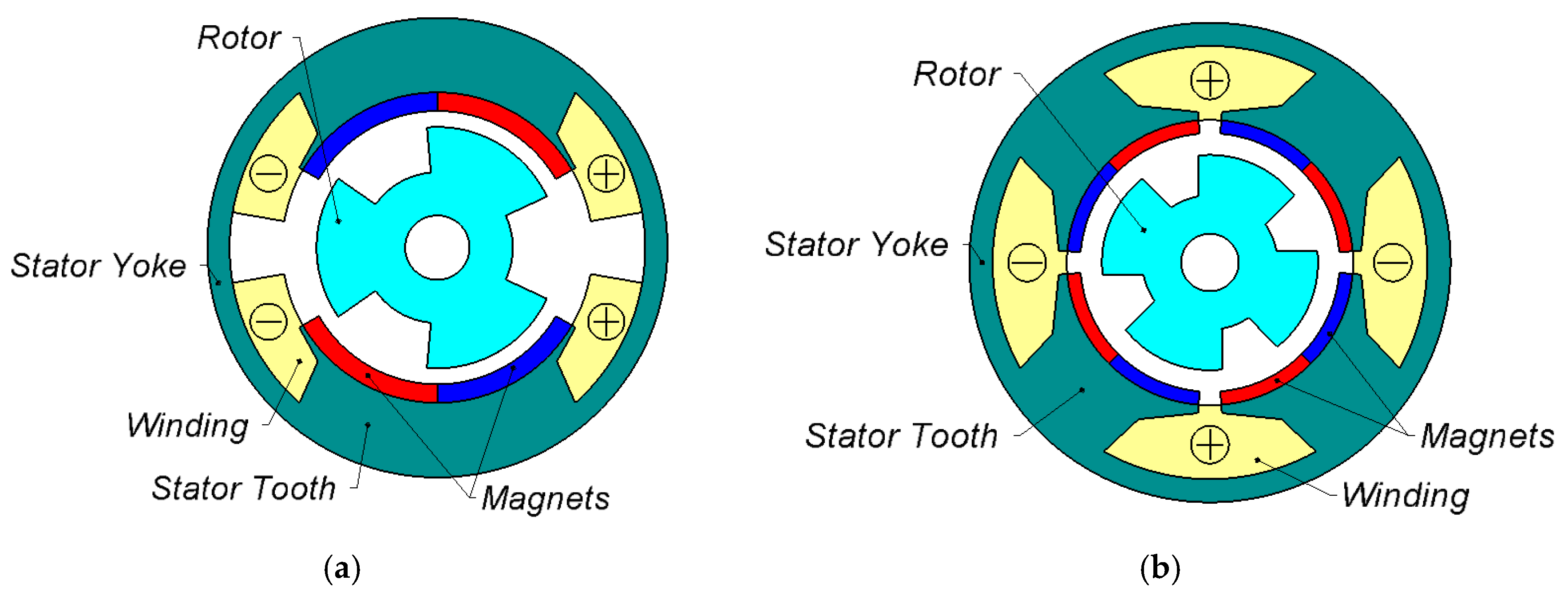
Flux Reversal Machines (FRMs) are doubly salient machines with permanent magnets (PMs) glued on the stator. The stator windings are of a concentrated type, and the flux linkage of the PMs reverses its polarity in the stator windings when the rotor rotates [1]. A first basic configuration of single-phase FRMs was described in [1] (Figure 1a). This FRM has a single phase, two stator teeth with two PM poles on each of them, and three rotor teeth. The FRM of this kind was designed for a high-speed vacuum cleaner [2]. Thanks to their geometry design, single-phase FRMs have several merits compared to the conventional permanent magnet synchronous machines (PMSMs), as follows: They are characterized with a simple and robust rotor structure due to the absence of PMs and windings in the rotor, which makes them easier for manufacturing and reduces their cost. Therefore, they can work properly and reliably in high-speed applications (over 10 krpm) [1,2,3,4,5]. However, the single-phase FRM design (Figure 1a), presented in [1,2], has the following disadvantages:

• Only two thirds of the stator internal surface are used, which decreases the power density and efficiency of the motor;
• There is no geometrical symmetry of rotating FRM as a whole by 180°, which causes radial force acting in the rotor. This radial force decreases the lifetime of the bearings and increases the acoustic noise and losses in the motor.

In this paper, in order to overcome the above disadvantages of the single-phase FRM shown in Figure 1a, a single-phase FRM shown in Figure 1b proposed in [3] is used to develop a three-phase FRM. A two-dimensional (2D) finite element model (FEM) is constructed to simulate the performance of the proposed motor. Furthermore, an optimization strategy based on the Nelder–Mead method is coupled with FEM to improve the performance of the proposed geometry.

The single-phase FRM prototype for the proposed FRM has four stator teeth, four rotor teeth, and two PM poles on each stator tooth as described in [3] (see Figure 1b). In contrast to the FRM described in [1], the nearest magnets mounted on the adjacent teeth are magnetized in the same direction. This FRM operates at a very high speed (about 28,000 rpm) as a drive of an angular grinder (power tool). The FRM prototype is described in [4]. In order to avoid the induced eddy currents in the magnets and the heating thereof, each magnet is divided into several electrically insulated segments.

Such single-phase FRMs have several [3] advantages compared to those of [1], as follows: (1) Increasing the power density and the efficiency because of better use of the stator surface; (2) the radial forces are absent, and the bearing lifetime is increased because of an even number of rotor teeth, resulting in motor symmetry.

Single-phase motors have a small starting torque and large torque ripple. It causes noise and vibrations, not only in the machine, but also in the mechanisms coupled therewith, and shortens their lifetime. Such machines have a limited range of applications, such as, for example, in circular saws, vacuum cleaners, fans, blowers, etc., in which a large starting torque is not required. In contrast, three-phase motors have a much lower torque ripple and can be used in a wide range of applications.

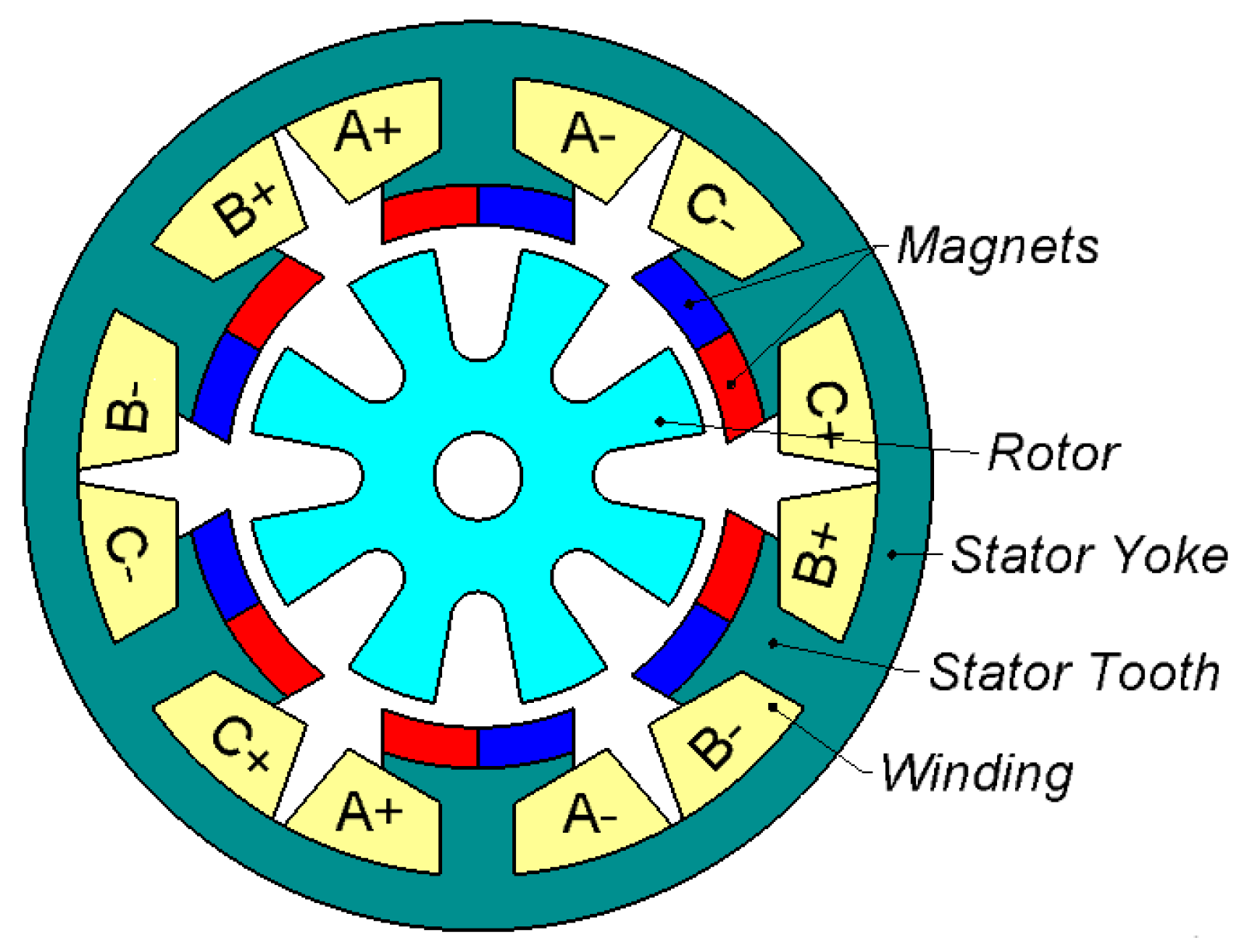
A three-phase FRM (Figure 2) is described in [6]. The FRM as a motor [6] operates from 180 rpm up to 18,000 rpm and has eight teeth on the rotor. The operating frequency is equal to 2.4 kHz at 18,000 rpm. Further increase of speed is complicated because of increasing the operating frequency. Besides, the three-phase FRM [7] is not used in industry, because of the following drawbacks: (1) The torque ripple is rather high (≈25%) [7] when a conventional three-phase frequency converter is used; (2) only two thirds of the stator internal surface are used, which decreases the power density and efficiency of the motor.

Therefore, the present paper discusses a novel three-phase high-speed modular design with four teeth on the rotor.

2. The Design of a New Three-Phase High-Speed FRM

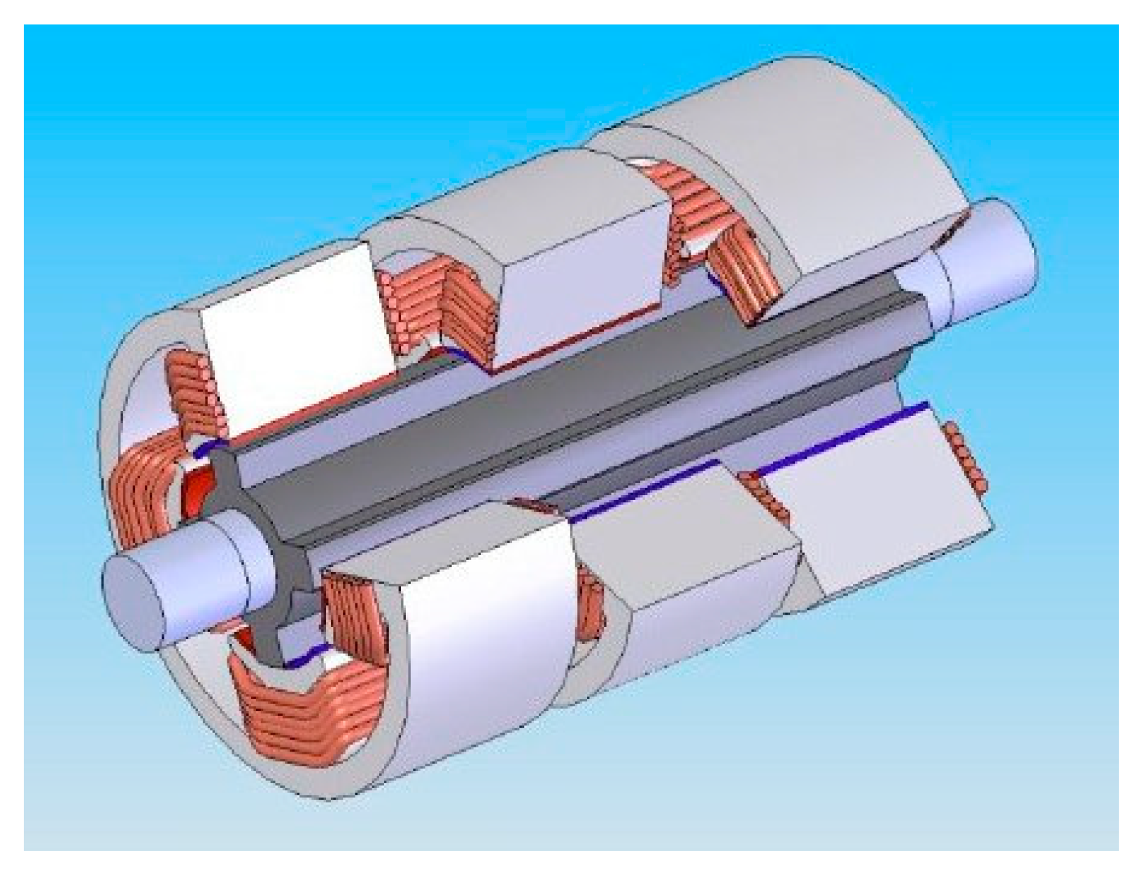
The present paper discusses a novel three-phase high-speed modular FRM, as sketched in Figure 3, that consists of three single-phase machines (Figure 1b). These three single-phase machines are mounted on a single shaft, shifted relative to each other by 120 electrical degrees (Figure 3). The proposed three-phase high-speed FRM is fed by a conventional three-phase frequency converter. The number of rotor teeth is reduced twofold compared to [6], which makes it possible to increase the upper limit of speed. Furthermore, the proposed FRM has low torque ripple compared to [6,7].

3. The Mathematical Model of the Single-Phase FRM

The three-phase FRM is composed of three single-phase FRMs in which the stator magnetic cores are separated from each other by the end winding parts, as well as insulation. Therefore, the electromagnetic coupling between the phases of the three-phase FRM can be considered as negligible.

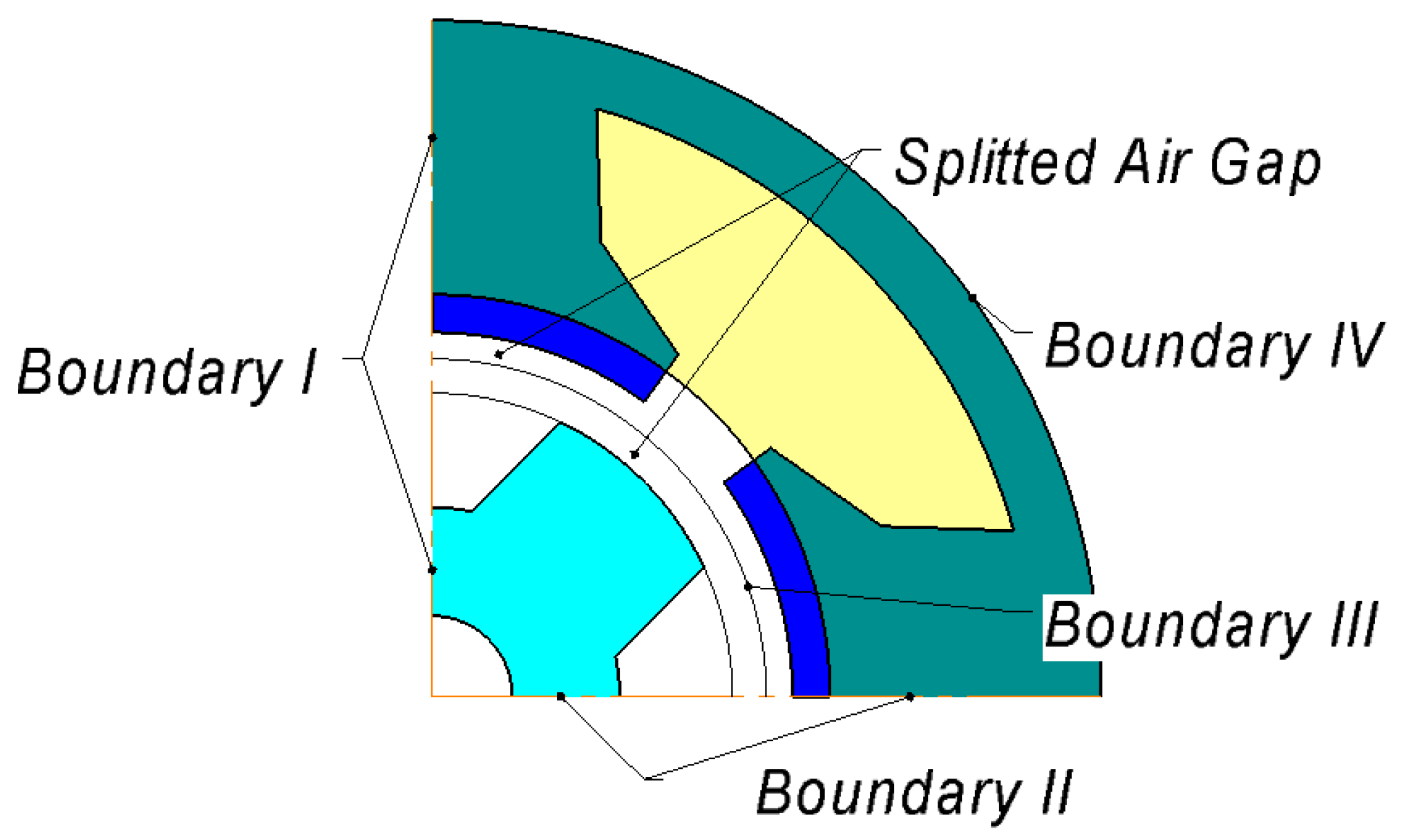
A detailed description of the mathematical model for the high-torque single-phase FRM powered by piecewise constant voltage is disclosed in [8]. The magnetic flux at different rotor positions is determined by integrating the voltage over time. Then, the 2D magnetostatic boundary problems are solved only for the actual pairs of the rotor position and the flux. Thanks to symmetry, the computational domain is reduced to a quarter. The computational domain is shown schematically in Figure 3. Boundaries I and II are joined with an aperiodic boundary condition. The boundary condition joining Boundary III takes into account the rotor position. In addition, the magnetostatic boundary problems can be solved only for the rotor positions in the range from 0 to 90°, which corresponds to the electric period.

In this paper, the mathematical modelling of the high-speed FRM is based on assuming a sinusoidal current waveform. Therefore, the 2D magnetostatic boundary value problems are solved for the current position pairs (Figure 4).

In this paper and in [8], the magnetic flux Φ and current density J are defined by the following expressions:

$$\mathsf{\Phi }=\frac{4LN}{S}{\displaystyle \iint }AdS$$

(1)

$$J=\frac{IN}{S}$$

(2)

where A is the z-component of the vector potential, L is the stack length of the magnetic cores, the integer 4 is used to account for the reduction of the computational domain, N is the number of turns in the slot, S is the slot area, and I is the current. The integration is carried out over the slot area.

Although in this paper and in [8], the same calculation area is used and the magnetostatic boundary problems are solved for the rotor positions of the same range, Equations (1) and (2) are treated differently in this paper compared to [8].

In [8], since the flux Φ is found by integrating the piecewise constant voltage and is considered to be given by solving the magnetostatic boundary problem for each rotor position, Equation (1) is treated as an additional equation, and the current defining the current density according to Equation (2) is taken as an additional variable.

In contrast to [8], herein the mathematical model is simplified by the fact that the currents are assumed to be predetermined and sinusoidal, and additional equations are not required. After solving the boundary value problem with the current density given Equation (2) for each rotor position, the fluxes Φ can be determined using the expression (1). Other aspects of the mathematical model, such as calculating the instantaneous torque of the single-phase FRM as well as the core and winding losses, are described in [8].

4. Torque and Line Voltage of Three-Phase FRM

During the rotation of the rotor of the single-phase FRM shown in Figure 1b, all electromagnetic processes are repeated after the rotor is rotated by 90 mechanical degrees. Therefore, 360 electric degrees corresponds to 90 mechanical degrees, i.e., one electrical revolution.

The three-phase FRM (Figure 3) consists of three single-phase machines rotated relative to each other by a third of the electrical period or by 30 mechanical degrees. After performing calculations for one single-phase machine, phase voltage and torque of two other single-phase machines can be obtained by shifting the waveform by a third of a period (120 electrical degrees). This shifting of the waveforms is particularly easy to be carried out when the number (n) of uniformly spread points on a period is a multiple of 3, i.e., n = 3k, where k is integer. In this case, the voltage and the torque of the other two machines are determined by making a phase shift for k and −k, respectively.

In the case of a Y-connection, the line voltage of the machine is determined by subtracting two phase voltage values. Owing to the fact that shifts do not alter the triplen harmonics, such harmonics are not present in the linear voltage. However, in particular, even harmonics can be present. Therefore, the positive and negative half-periods of the line voltage waveform may not coincide entirely. In particular, maximum voltage value and minimum voltage value may not match. This will be seen later.

The three-phase machine torque is determined as the sum of the torques of the three single-phase machines. Therefore, the period of the torque waveform equals to one third of the electric period or, in other words, only triplen harmonics are existing in the torque waveform.

Although the calculation of the torque waveform of the three-phase FRM is fully based on the calculation of the torque waveform of the single-phase FRM, the former requires more computational efforts than the latter. The torque waveform period of the three-phase FRM is three times as short as that of the single-phase FRM and is represented with three times less the points. In this study, to obtain 15 points per period of the three-phase FRM, 45 points per period of the single-phase FRM are taken. Therefore, 46 boundary problems are solved: 44 boundary problems inside the electric period and two boundary problems at its ends.

5. Optimization of the FRM Design

Multi-objective optimization most fully meets the requirement of designing the three-phase high-speed FRM for a real application [9]. Some multi-objective methods are aimed to build the Pareto front, that is, the set of the solutions in which no objective can be improved without worsening other objectives. In this case, the engineer chooses such a solution among the Pareto front in which the objectives reach their values according to their merits in the given task. Usually, such an approach requires a large number of function calls (3000 as reported in [9]).

Another approach to multi-objective optimization is implemented on the basis of the one-criterion methods of optimization. In this case, the objectives merits should be set to construct the optimization criterion as a function of these objectives. It is possible to use both encouraging and fining components of this function [10].

Therefore, for any multi-objective optimization to be implemented, the objectives’ merits must be set either at the optimization beginning or at its end.

To reduce the calculation efforts, the multi-objective optimization implemented on the basis of the one-criterion Nelder–Mead method is used in the paper. Such an approach for the optimization of the high-speed single-phase FRM is developed in [5]. In contrast to the approach described in [9] and requiring a large number of function calls (3000), the optimization based on the Nelder–Mead method requires only 115 function calls [5], which is 26 times lower.

Since the Nelder–Mead algorithm is well known and it is also implemented in the Matlab function “fminsearch”, we do not include a detailed description about the algorithm in the paper.

As for the number of individuals, the Nelder–Mead algorithm can be considered as the algorithm of the group behavior. In contrast to a genetic algorithm where the most adapted individual wins, the Nelder–Mead algorithm improves the weakest individual. The number of vertexes in the simplex (the number of individuals) is n + 1, where n in the dimension of the parametric space. In our case, n = 7, and the number of individuals is 8.

The three-phase high-speed FRM is optimized for a fan load in which the load torque of the machine is proportional to the rotational speed in a quadratic way. Herein, the optimization process is performed according to several criteria, and thus, the objective function is formulated based on such criteria. The Nelder–Mead method used for the optimization [11] is a gradient-free method of unconditional optimization of a function of several variables. The method is easily applicable to non-smooth and/or noisy functions [12]. This method is widely used for non-linear optimization and is well suited for problems in which the derivatives of functions may be unknown. The Nelder–Mead method can be more effective than gradient-based methods, as well as some other gradient-free methods; in particular, the Powell method [12].

Four optimization criteria are discussed in detail below. To add, the merits of the criteria are set, which is necessary to determine the objective function.

5.1. Loss Reduction in a Wide Speed and Torque Range

Pumps, fans, compressors, blowers, etc. are often operated at a partial load. Therefore, the motor must be calculated in three different modes shown in

Table 1. The torques and the speeds given in % of rated values in three modes.

Mode	Speed (%)	Torque (%)
1	50	25
2	75	50
3	100	100

. The modes are approximately corresponding to the quadratic speed dependence of the torque. Let us assume that in a wide range of powers, periods of work within different power values are equal. Therefore, this criterion is based on motor losses over the whole time length of a period, as follows:

$$K_1=1-\eta$$

(3)

$$\eta =\frac{{{\displaystyle \sum }}_{i=1}^{3}P{M}_i}{{{\displaystyle \sum }}_{i=1}^{3}P{A}_i},$$

(4)

where PM_i is the mechanical power of the motor, and PA_i is the electrical active power of the motor. Mechanical losses, such as ventilation loss and bearing loss, are ignored.

Use of the criterion $K_1$ requires approximately three times as many calculations of FRM modes per the calculation of the objective function as the optimization, based on only one rated mode. However, this provides significantly higher averaged efficiency at a wide range of load powers.

This criterion K₁ is considered as the base criterion, and the significance of other criteria is evaluated in comparison with this criterion.

5.2. Required Converter Power

The converter of the FRM is selected based on the maximum voltage and current, i.e., kVA rating. Due to the presence of even harmonics in the FRM voltage range, the maximum and minimum voltage values may not match. Since the highest current value and the highest voltage value are reached in nominal mode (mode 3), the second optimization criterion is:

$$K_2=3\frac{\max \left(I_3\right)}{\sqrt{2}}\frac{\max \left(\left|U_3\right|\right)}{\sqrt{6}}$$

(5)

where I₃ is the phase current, and 3 is the line voltage. The modulus sign is used to denote that the maximum and minimum voltage values may not match.

The merit of the K₂ criterion is considered equal to the merit of the K₁ criterion in that a 1% increase in K₁ is considered a fair trade-off for a 1% decrease in K₂, and vice versa. K₂ matches the apparent power in the case of sinusoidal voltages and currents and is expressed through the maximum instantaneous voltage, which is the convertor limitation.

5.3. Torque Ripple in the Three-Phase Machine in a Wide Range of Loads

Torque ripple causes vibrations not only in the machine, but also in the mechanisms coupled therewith, thus creating acoustic noise. In order to ensure low noise level and low torque ripple in a wide range of loads, the following criterion is proposed:

$$K_3={\displaystyle \sum }_{i=1}^{3}TR{3}_i$$

(6)

where TR3_i is the peak-to-peak torque ripple value for a three-phase machine in various modes, expressed as the percentage of mean torque in the corresponding mode.

The merit of this criterion is considered to be half of the merits of the first two criteria. In other words, their 1% loss increase is a fair trade-off for a K₃ decrease of 2%.

5.4. Torque Ripple in the Single-Phase Machine in A Wide Range of Loads

Torque ripple in the single-phase machines that constitute the three-phase machine can create additional loads on the single-phase machines, as well as a certain noise level increase, due to vibrations inside these machines. Therefore, a fourth criterion similar to K₃ is introduced, wherein TR3_i is replaced by torque ripple of the single-phase machine TR_i:

$$K_4={\displaystyle \sum }_{i=1}^{3}T{R}_i.$$

(7)

However, the merit of this criterion is much lower compared to the value of K₁, K₂. An increase in any of the criteria K₁, K₂ by 1% is permissible only if a decrease in K₄ by approximately 10% is provided.

5.5. Optimization Procedure

The Nelder–Mead method is used in this work to minimize the objective function according to the criterion merits described before:

$$F=K_1{K}_2\sqrt{K_3}{K}_4^{\frac{1}{10}}$$

(8)

This expression means that the following improvements of the objectives are equally valuable: Decreasing K₁ by 1%, decreasing K₂ by 1%, decreasing K₃ by 0.5%, and decreasing K₄ by 0.1%.

Implementing the optimization procedure based on the one-criterion method is justified by significant efforts required for computing the objective function (8): Three modes must be calculated for each objective function call, and the large number of the rotor position must be taken into account.

Not all criteria will be improved after carrying out the optimization procedure. The value of a criterion may increase if it is considered to be a fair trade-off for lowering other criteria. This does not mean that the presence of increasing criteria in the objective function is useless, as their absence in the objective function could have led to their even greater increase.

This paper describes simulation and optimization of a three-phase FRM (4.5 kW, 28,000 rpm) consisting of three single-phase motors of 1.5 kW each.

Table 2. Fixed geometrical parameters of the FRM.

Parameter	Value
The stator outer diameter, mm	54
The rotor shaft diameter, mm	7
Single-phase FRM stack length, mm	40
The rotor slot bottom diameter, mm	14
The magnet thickness, mm	1.4
The air gap, mm	0.4

shows the geometrical parameters of the FRM, which are constant during optimization process.

In order to reduce eddy loss in the permanent magnets, each magnetic pole is divided into 8 electrically insulated segments in the azimuthal direction. The residual flux density (B_r) and the coercivity (H_cj) of the permanent magnet are 1.2 T and H_cj = 1000 kA/m, respectively. In practice, PMs having a greater residual flux density, e.g., B_r = 1.3 T, may be necessary due to the presence of insulating gaps between magnets.

The M350-50A steel grade is selected for both the stator and the rotor. Steel sheet thickness is 0.5 mm.

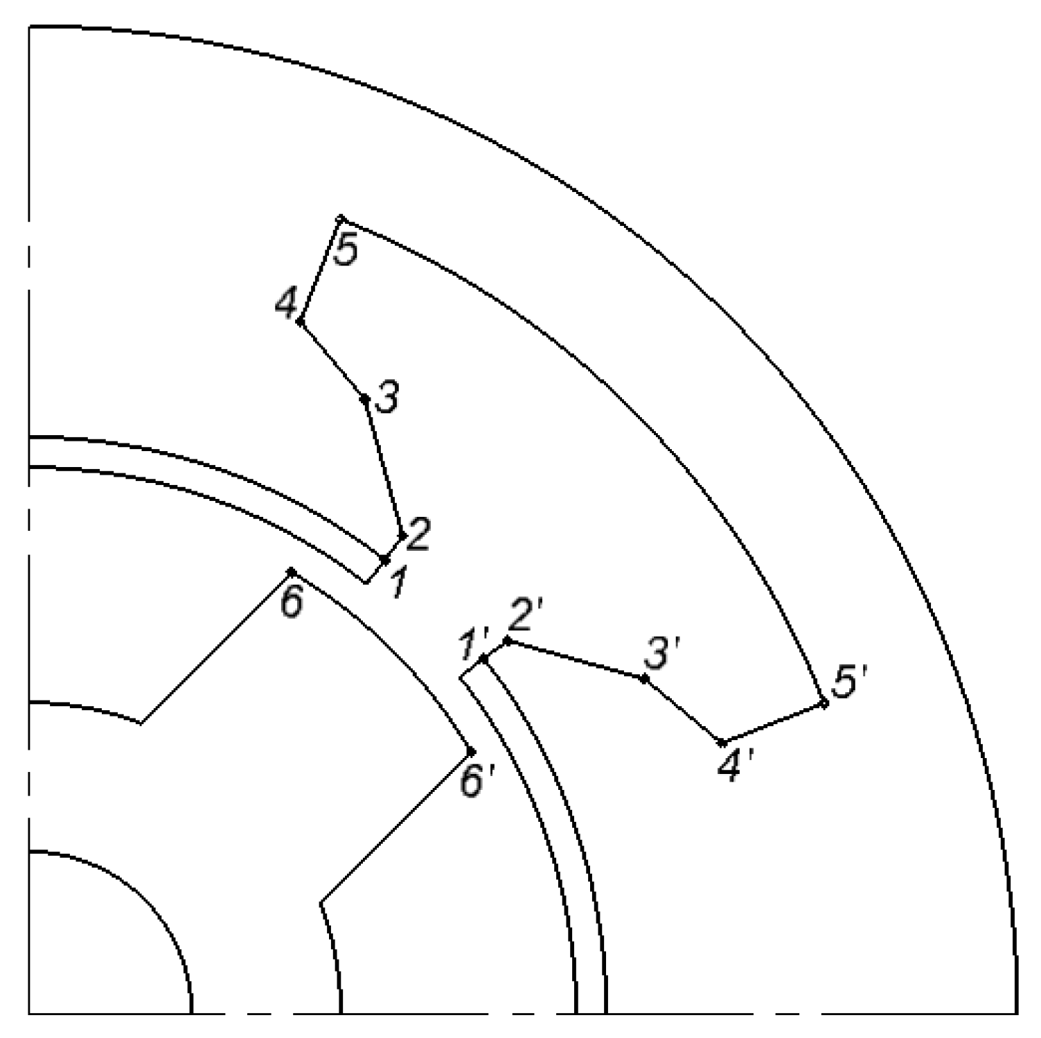
Figure 5 displays the detailed slot geometry. The slot opening is smoothed with small segments 1–2 and 1′–2′. The segments 4–5 and 4′–5′ represent the teeth legs and are radii. The lines 2–3–4 and 2′–3′–4 approximate an Archimedes helix.

Let’s introduce the following notation:

• Radius values R₁, R₂, R₃, R₄, R₅ of the stator slot points 1, 2, 3, 4, 5;
• α₁, α₂, α₃, α₄, α₅ are the angular distances between points 1 and 1′, 2 and 2’, 3 and 3’, 4 and 4’, 5 and 5′ of the slot;
• α₆ is the angular distance between points 6 and 6’ of the rotor teeth.

Therefore, the following constraints are imposed on the parameters:

$$\begin{gathered} R_2=R_1+0.7mm, \\ {R}_3=(R_2+R_4)/2 \\ {\alpha }_2={\alpha }_1 \\ {\alpha }_3=({\alpha }_2+{\alpha }_4)/2 \\ {\alpha }_4={\alpha }_5 \end{gathered}$$

(9)

The geometrical parameters R₁, R₄, R₅, α₁, α₅, α₆, which are independent according to (9), are adopted as optimization parameters.

In this paper, the current angle, which is the angle between the current vector and the rotor position, is assumed to be zero when at rotor position of phase A, illustrated in Figure 4. The phase current A takes its maximum value, and the current sign is chosen so as to provide the positive torque. In the underload modes (Mode 2 and Mode 1), the current angle is chosen to be zero.

Apart from the geometrical parameters and constrains, the current angle in Mode 3 is also used as another parameter in the optimization of FRM. This is because in the field weakening mode, the current angle varies the required converter power. Furthermore, it varies magnetic field oscillations in the cores and current and, consequently, the core and the winding losses, hence the motor efficiency.

6. Optimization Results and Discussion

The optimization process, using the optimization procedure presented in the previous section, was applied to the 2D FEM. The DC bus voltage and the fundamental frequency at the rated value are 560 V and 1867 Hz, respectively. The optimization was stopped after 128 objective function calls. At that, the ratio of the maximum value of the objective function in the simplex to the minimum one is less than 0.5%.

Some motor characteristics before and after the optimization are provided in

Table 3. FRM characteristics before and after optimization.

Parameter	Before	After
The stator inner diameter, mm	27.6	29.5
Input torque at rated speed, N∙m	1.53	1.53
Number of turns in the slot	47	50
Current at rated mode, RMS, A	11.4	9.7
Efficiency at mode No. 1, %	88.4	87.4
Efficiency at mode No. 2, %	90.4	89.7
Efficiency at mode No. 3, %	90.3	90.1
η, %	90.2	89.8
TR31, %	231	38.6
TR32, %	117	21.5
TR33, %	63.4	14.5
TR1, %	827	768
TR2, %	411	424
TR3, %	282	291
Required convertor power $(K_2)$, kW	7.78	6.61
Objective function ($F$), W	1431.7	823.09

.

In Table 3, TR3_i is torque ripple in the three-phase FRM, i stands for the different modes, and TR_i is torque ripple in the single-phase FRM.

The optimization criteria values, as well as the logarithm of the ratios before and after optimization, are shown in

Table 4. Optimization criteria.

Parameter	Before	After	Log (after/before)
K1	0.09839	0.10238	0.04
K2, W	7780	6610	−0.163
K3	2.03	0.863	−0.855
K4	15.2	14.8	−0.027
Objective function, W	1431.7	823.09

. The logarithm is used to account for the “compound interest effect.”

As a result of optimization, the K₁ optimization criterion increased by about 4%, which resulted in a slight decrease in efficiency. However, a significant reduction in torque ripple in the three-phase FRM was achieved. Other optimization parameters also yielded some improvements.

The drop in efficiency as a result of optimization is more pronounced under a reduced load compared to the nominal mode. This effect is explained by the fact that the contribution of the average (over a lengthy time period) mechanical and electric power values at underload is lower compared to the rated mode. When another K₁ criterion is selected, the optimization result can be different.

Torque ripple in the three-phase machine is significantly reduced (by more than four times for all three modes), which justifies a certain decrease in efficiency.

Torque ripple in the single-phase machine is increased somewhat in modes 2 and 3; however, taking into account the reduction in the same parameter at the most under-loaded mode, the K₄ criterion is also reduced.

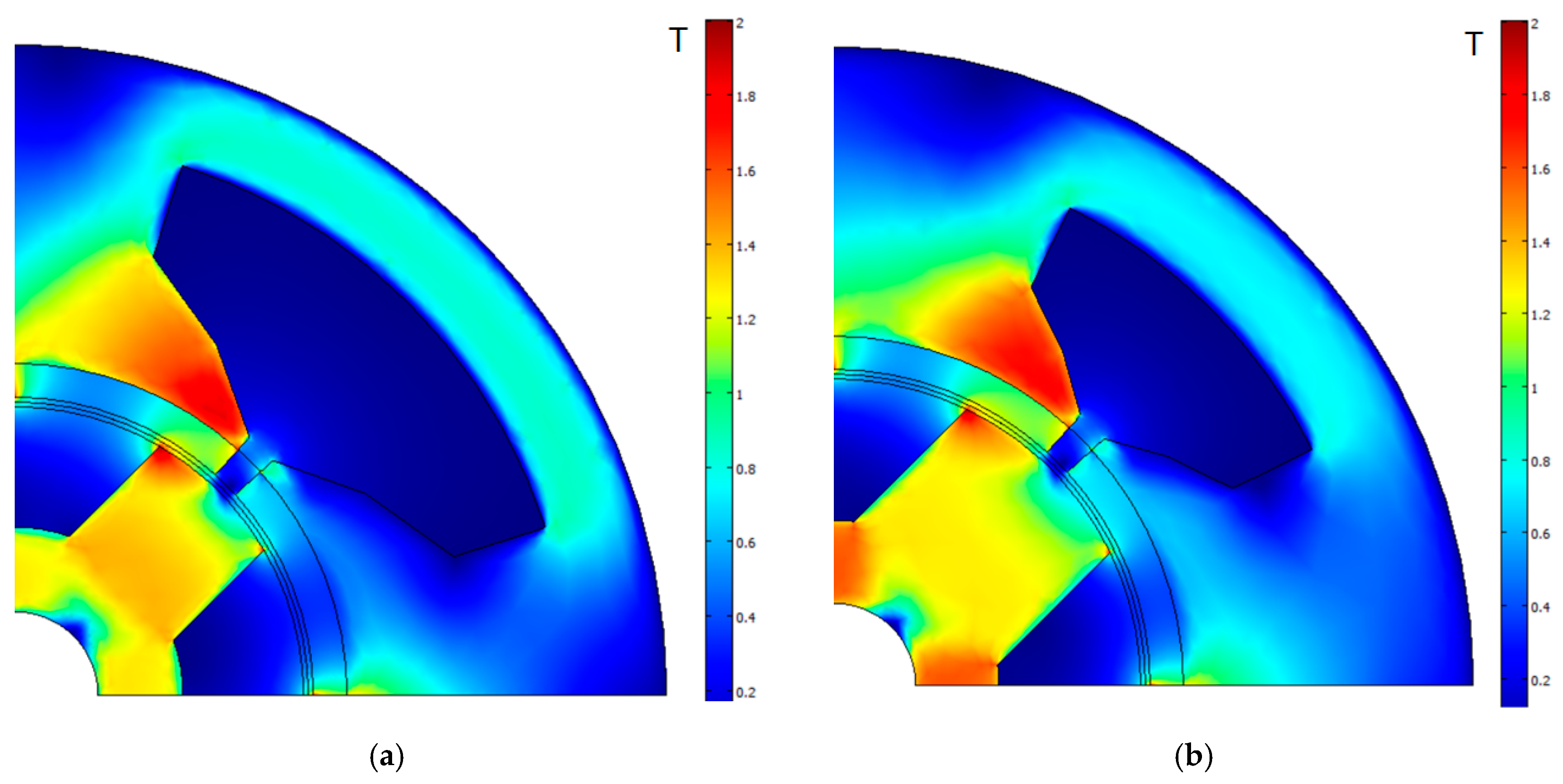
Figure 6 shows the FRM geometry and magnetic flux density at the rated mode before and after optimization. The position of the rotor when the rotor tooth is located in front of the stator slot opening is obvious in Figure 6. Both PM poles shown in the figure are magnetized equally in the same direction. However, the current flowing through the winding amplifies one magnetic pole and weakens the other magnetic pole. The rotor rotates in the direction of the strongest magnetic pole. A similar situation occurs when rotor teeth are located in front of the middle part of the stator teeth, i.e., over the junction of magnetic poles of different polarities.

The FRM before and after optimization has roughly the same mass as indicated in

Table 5. Active material masses of the three-phase FRM before and after optimization.

Parameter	Before	After
The stator core mass, kg	1.1	1.2
The rotor core mass, kg	0.22	0.3
The core winding mass, kg	0.5	0.293
The magnets mass, kg	0.096	0.103
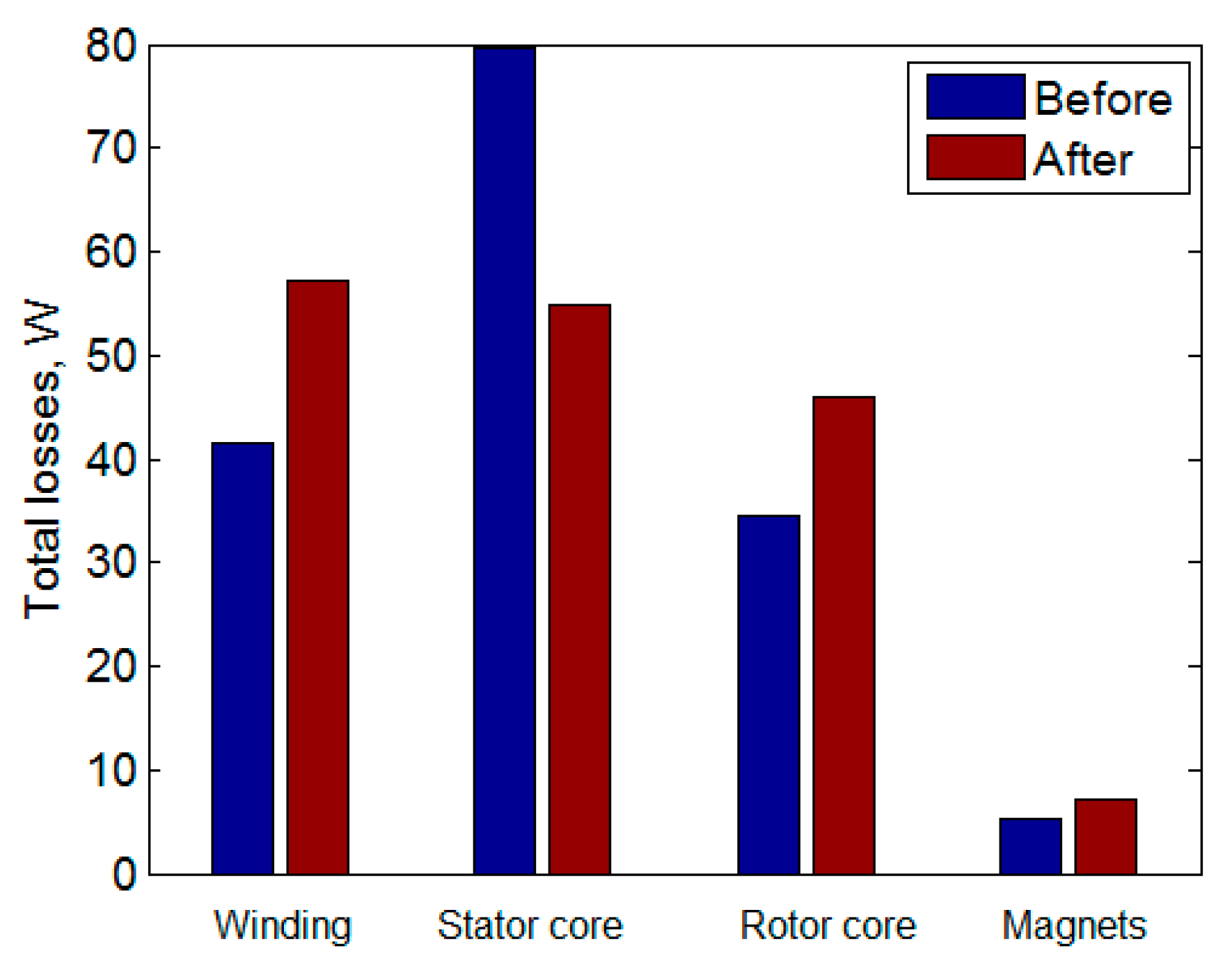
Total active mass, kg	1.91	1.9

. The increased mass of the rotor and the stator magnetic cores is compensated by the decrease in winding mass. During the optimization, the slot shape became more rounded, which reduced the slot scattering field and the saturation of the machine, and increased its power factor. Furthermore, the stator yoke length is decreased, which decreased the stator core losses and compensated an increase in winding losses.

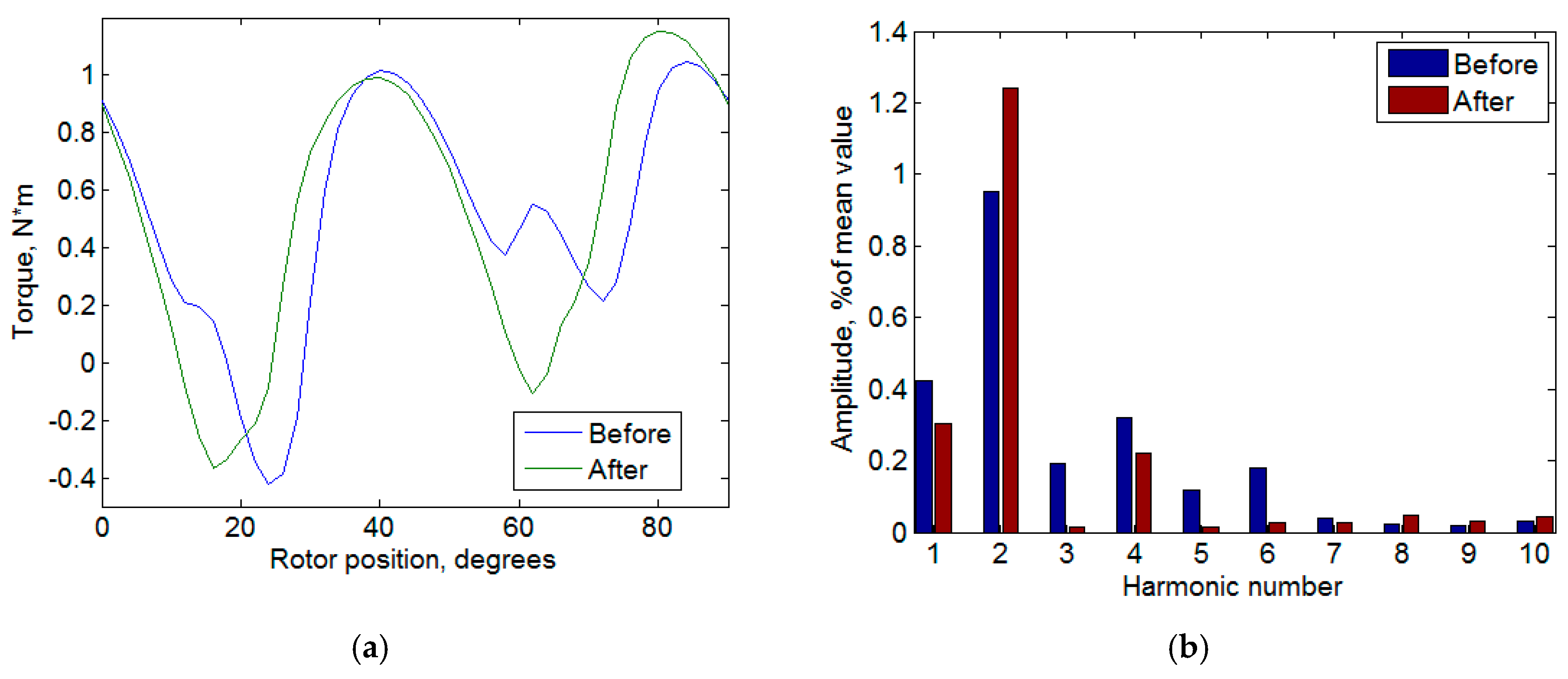
Figure 7 shows the losses in various parts in the FRMs at rated power. Figure 8 reports the torque ripple and its harmonic spectrum of the single-phase FRM at the rated mode. It is obvious that the first harmonic is reduced, while the second harmonic is increased more significantly after the optimization. As a result, torque ripple is slightly increased. Triplen harmonics (third and sixth) are significantly suppressed. As for the next triplen harmonic (ninth), its value is very small in both cases. Triplen harmonic suppression results in decreasing the torque ripple of the three-phase machine.

Figure 9 shows the torque ripple curves of the three single-phase machines. The blue line in Figure 9 corresponds to the portion of the graph (Figure 8a) in the range from 0 to 30° that belongs to the first single-phase FRM. The green line corresponds to a portion from 30° to 60° that belongs to the second single-phase FRM. The red line corresponds to a portion from 60° to 90° that belongs to the third single-phase FRMs. The combined image of the blue, green, and red lines following each other forms the graph for a single-phase FRM, as shown in Figure 8a.

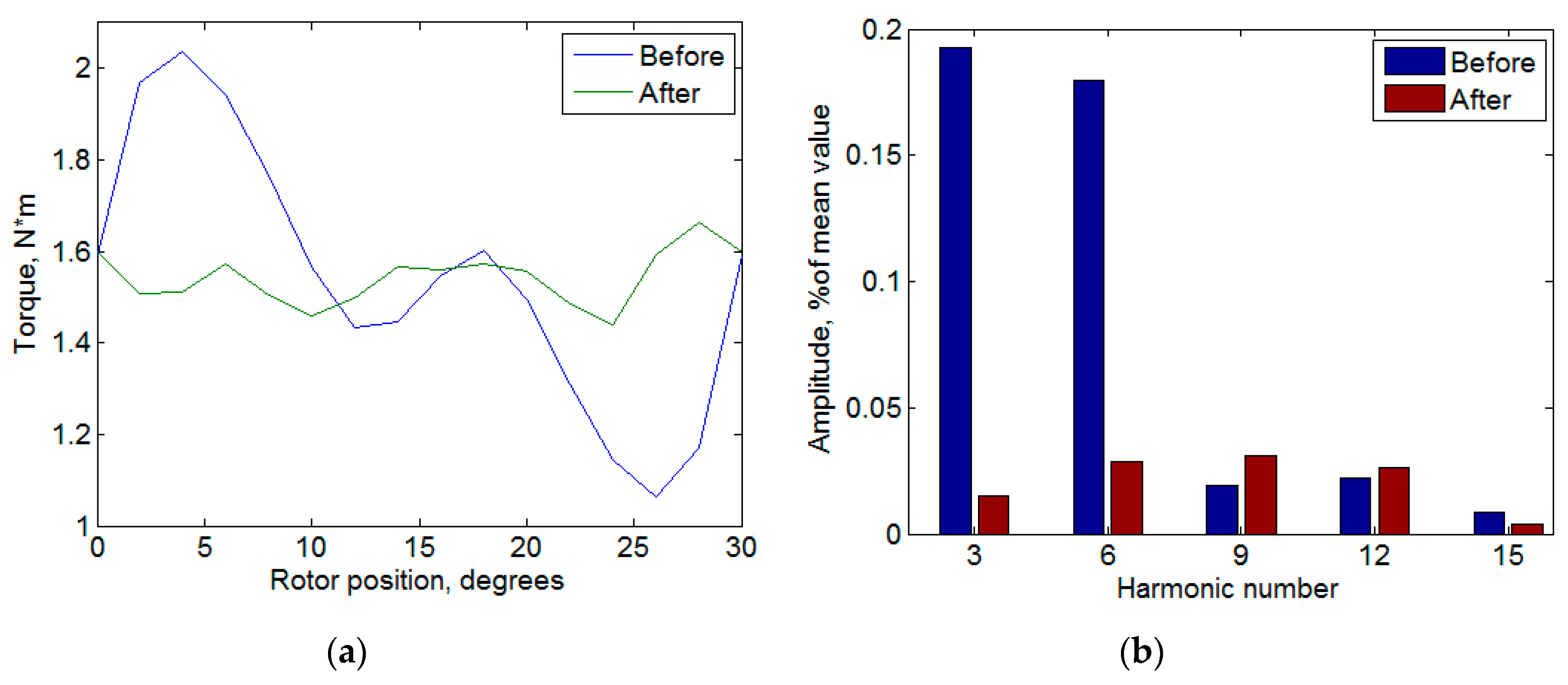
The torque ripple of the three-phase FRM composed of the three single-phase FRMs has a period of 30°. The total torque of the three-phase FRM (defined as the sum of the three graphs (Figure 9) is shown in Figure 10a. Figure 10b shows the triplen harmonics of the three-phase FRM. Evidently, the torque ripple is reduced significantly after the optimization.

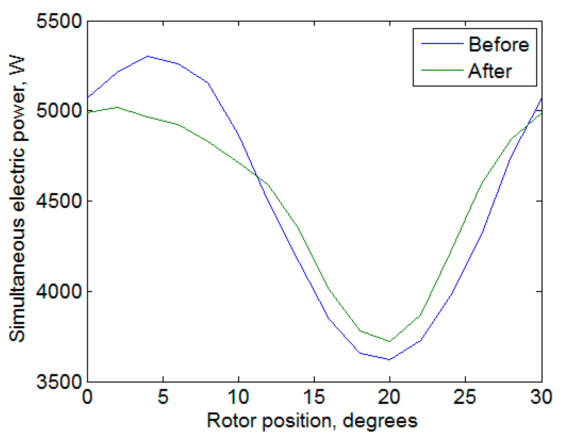
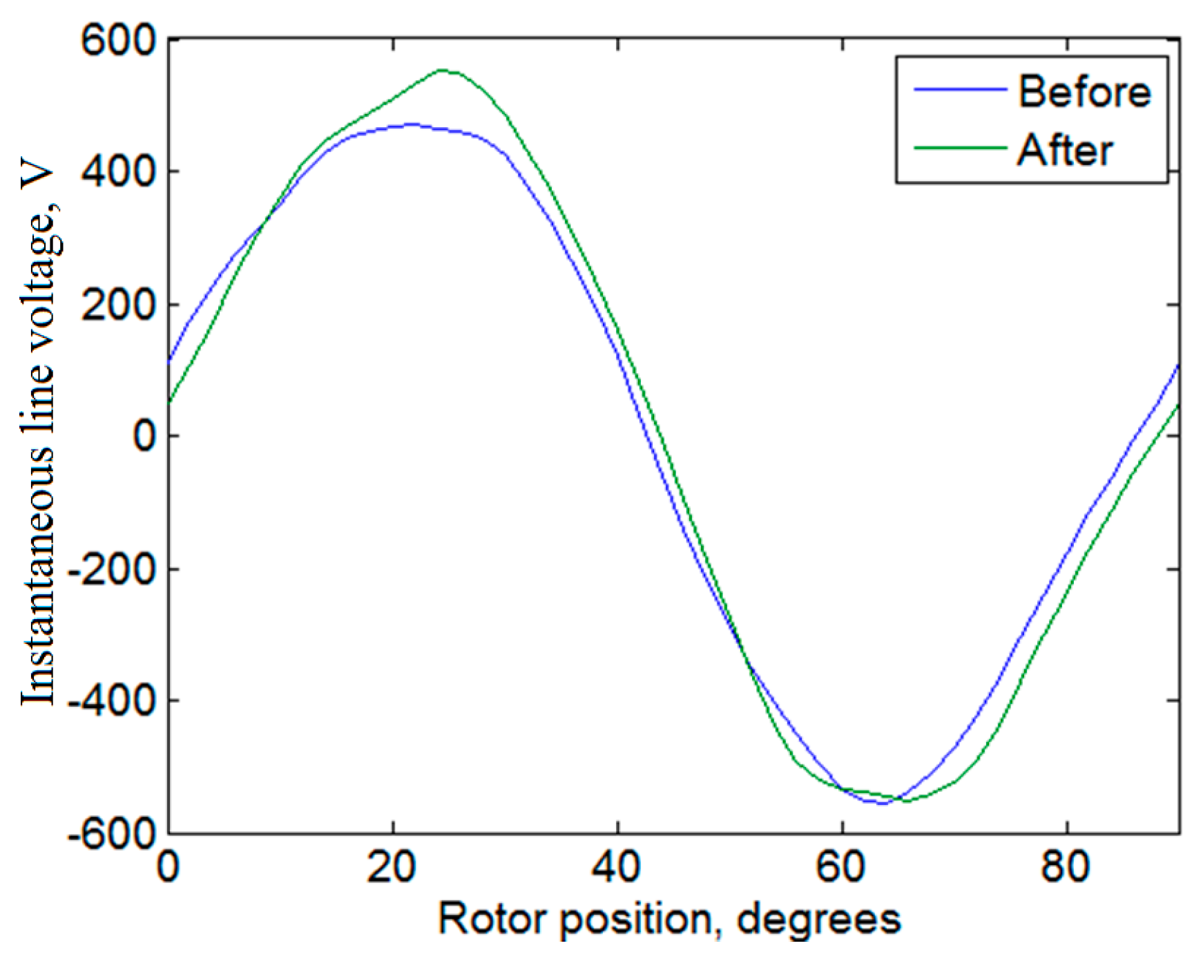
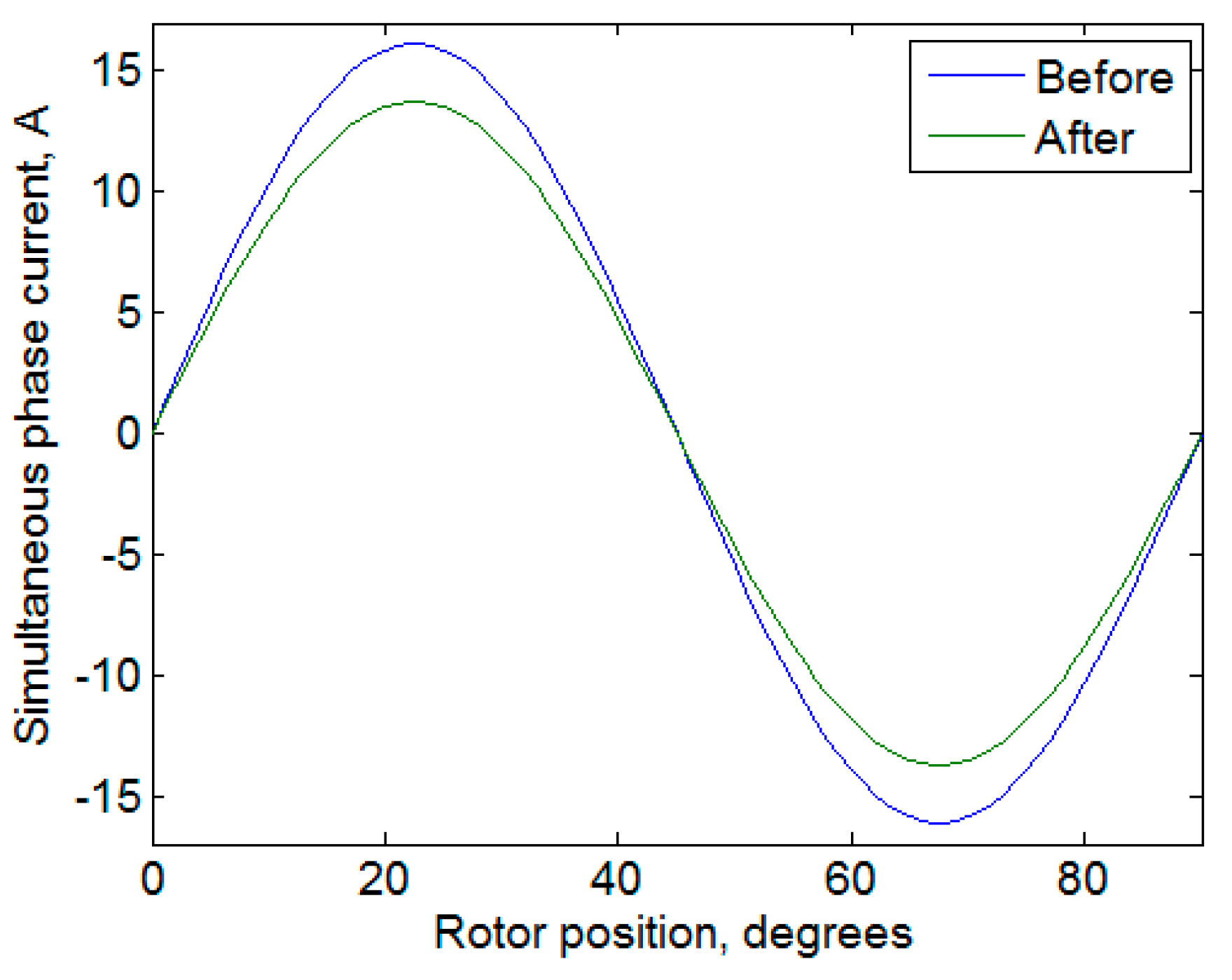
Figure 11, Figure 12 and Figure 13 illustrate the waveform of FRM line supply voltage, current, and instantaneous power, before and after optimization.

As a result of optimization, the voltage waveform is less sinusoidal, which could be due to THD not being considered as part of the target function. However, it should be noted that a more complete use of voltage is in evidence. Before the optimization, the maximum voltage is 469 V, and the minimum voltage is −554 V. A converter for the FRM before the optimization should be selected based on maximum voltage magnitude, and therefore, the positive half-wave is underused. After the FRM optimization, the maximum and minimum voltages are 552 V and −552 V, i.e., the values are equal in magnitude. Furthermore, sinusoidal current amplitude was decreased from 16.1 A to 13.7 A. This results in a 15% decrease in the required converter power.

7. Conclusions

In this article, the design of a novel three-phase FRM composed of three single-phase machines is presented. A combined mathematical modelling and optimization technique was carried out. The three-phase FRM torque waveform contains only triplen harmonics, while its line voltages’ waveform contains only non-triplen harmonics. At the optimization, the FRM torque ripple is reduced from 63.4% to 14.5% at the rated mode. Furthermore, the required converter power is decreased by 15%. Other objectives are changed negligibly. However, including these objectives in the objective function prevents their unacceptable worsening during optimization to achieve greater improvement in other ones.