Reliable Design for a Network of Networks with Inspiration from Brain Functional Networks

Abstract

In realizing the network environment assumed by the Internet-of-Things, network slicing has drawn considerable attention as a way to enhance the utilization of physical networks (PNs). Meanwhile, slicing has been shown to cause interdependence among sliced virtual networks (VNs) by propagating traffic fluctuations from one network to others. However, for interconnected networks with mutual dependencies, known as a network of networks (NoN), finding a reliable design method that can cope with environmental changes is an important issue that is yet to be addressed. Some NoN models exist that describe the behavior of interdependent networks in complex systems, and previous studies have shown that an NoN model based on the functional networks of the brain can achieve high robustness, but its application to dynamic and practical systems is yet to be considered. Consequently, this paper proposes the Physical–Virtual NoN (PV-NoN) model assuming a network-slicing environment. This model defines an NoN availability state to deal with traffic fluctuations and interdependence among a PN and VNs. Further, we assume three basic types of interdependence among VNs for this model. Simulation experiments confirm that the one applying complementary interdependence inspired by brain functional networks achieves high availability and communication performance while preventing interference among the VNs. Also investigated is a method for designing a reliable network structure for the PV-NoN model. To this end, the deployment of network influencers (i.e., the most influential elements over the entire network) is configured from the perspective of intra/internetwork assortativity. Simulation experiments confirm that availability or communication performance is improved when each VN is formed assortatively or disassortatively, respectively. Regarding internetwork assortativity, both the availability and communication performance are improved when the influencers are deployed disassortatively among the VNs.

1. Introduction

The Internet-of-Things (IoT) has seen an increasing number of practical implementations in recent years, regarding not only traditional Internet services but also other services of extreme societal importance, such as infrastructure (e.g., electricity grids, vehicular traffic) and life-critical services (security, medical treatment, etc.) [1,2]. This situation is leading to the emergence of interconnected networks with mutual dependencies, known as a network of networks (NoN) [3]. Network slicing based on network virtualization technology can be regarded as an NoN case and has been attracting much attention as a way to realize the assumed IoT network environment [4,5]. In this architecture, sliced networks, i.e., virtual networks (VNs), are created by service providers to offer specific services on physical networks (PNs) provided by the infrastructure providers. To enhance the flexibility and efficiency of resource utilization, recent studies have investigated new methods for reallocating resources dynamically between VNs according to traffic fluctuations instead of dividing the PN resources statically [6,7,8,9]. However, although the above methods have several advantages, traffic fluctuations in one VN can be propagated to other VNs because of the mutual dependences between the VNs sharing the same PN resources [10,11]. In the upcoming IoT network scenario, environmental changes in service networks will exert an increasing influence on society and human life. Consequently, an urgent issue is to establish a method for designing an NoN with high reliability, namely, the ability to sustain network services under traffic fluctuation, assuming the network-slicing environment.

The Catastrophic NoN (C-NoN) was presented as a model expressing NoN availability based on actual interconnected networks comprising infrastructure networks in Italy, namely, a power network and a control network [12]. The functional availability of each infrastructure network depends on that of the other network: the power network must be operated by the control network, while the control network must be supplied with electricity by the power network. The C-NoN model reproduces the dependence between both networks, revealing how partial fluctuations spread their influence over the entire NoN.

On the other hand, Morone et al. argued that not all complex networks existing in nature are vulnerable to fluctuations [13]. Brain functional networks comprise a number of mutually connected network modules (i.e., regions) of neural cells. The regions are interdependent to complement their functionalities. Advances in neuroimaging technology, such as functional magnetic resonance imaging (fMRI), now make it possible to identify the interregional dependence of brain functional networks, for which Morone et al. proposed the Brain NoN (B-NoN) model [13]. The B-NoN model reproduces the complementary interregional dependence and elucidates the mechanisms that suppress the propagation of local fluctuations. However, insights from studying NoN models are yet to be applied to practical systems of information networks including the aforementioned network-slicing environment.

As an NoN system, we consider herein layered VNs with slicing, and we propose the Physical–Virtual NoN (PV-NoN) model based on existing NoN models. To deal with traffic conditions and interdependence among a PN and VNs, this model describes NoN availability, focusing on the states of the node interfaces. Here, availability denotes the ability for a network to transmit packets without loss from the source to the destination. For the PV-NoN model, we assume three different types of interdependence according to how the resources (e.g., packet buffer, network I/O) are assigned on the physical interfaces. To investigate NoN reliability, we measured availability and communication performance through simulation experiments. We confirm that among the three types of PV-NoN models, the one based on the B-NoN model, which reproduces the complementary interdependence of brain functional networks, achieves high availability and communication performance while preventing interference among the VNs.

We also investigate a method for designing reliable network structures in the PV-NoN model. To this end, we configure the deployment of network influencers, which are the network components whose fluctuations have the largest influence on the entire network [14,15,16], from the perspective of inter/intranetwork assortativity. Assortativity is a network metric for evaluating the correlation of node centrality, i.e., node influence [17]. Evaluation results show that configuring the assortativity within each VN and among the VNs can improve NoN availability and communication performance. Obtaining guidelines on influencer design with the PV-NoN model contributes directly to controlling the performance of network slicing under unpredictable environmental changes, thereby leading to the design of highly reliable interdependent network architectures in future IoT scenarios. Our results also suggest the potential of the NoN model to be applied to other interconnected network systems wherein there is mutual internetwork dependence.

2. Basic Principles of NoN Models

There have been several studies that theoretically investigate structural and behavioral performance of NoN [18,19,20,21,22]. However, in recent years, Morone et al. proposed a model that deals with the interdependency of NoN [13], and there has been no study that investigates the application of the models into information networks, including virtualized network environment, where physical resources are virtually partitioned. Therefore, we introduce the general concepts of NoN models and provide the definitions of the B-NoN and C-NoN models for the fundamental of our proposed model. We also explain the method for detecting network influencers based on the NoN models.

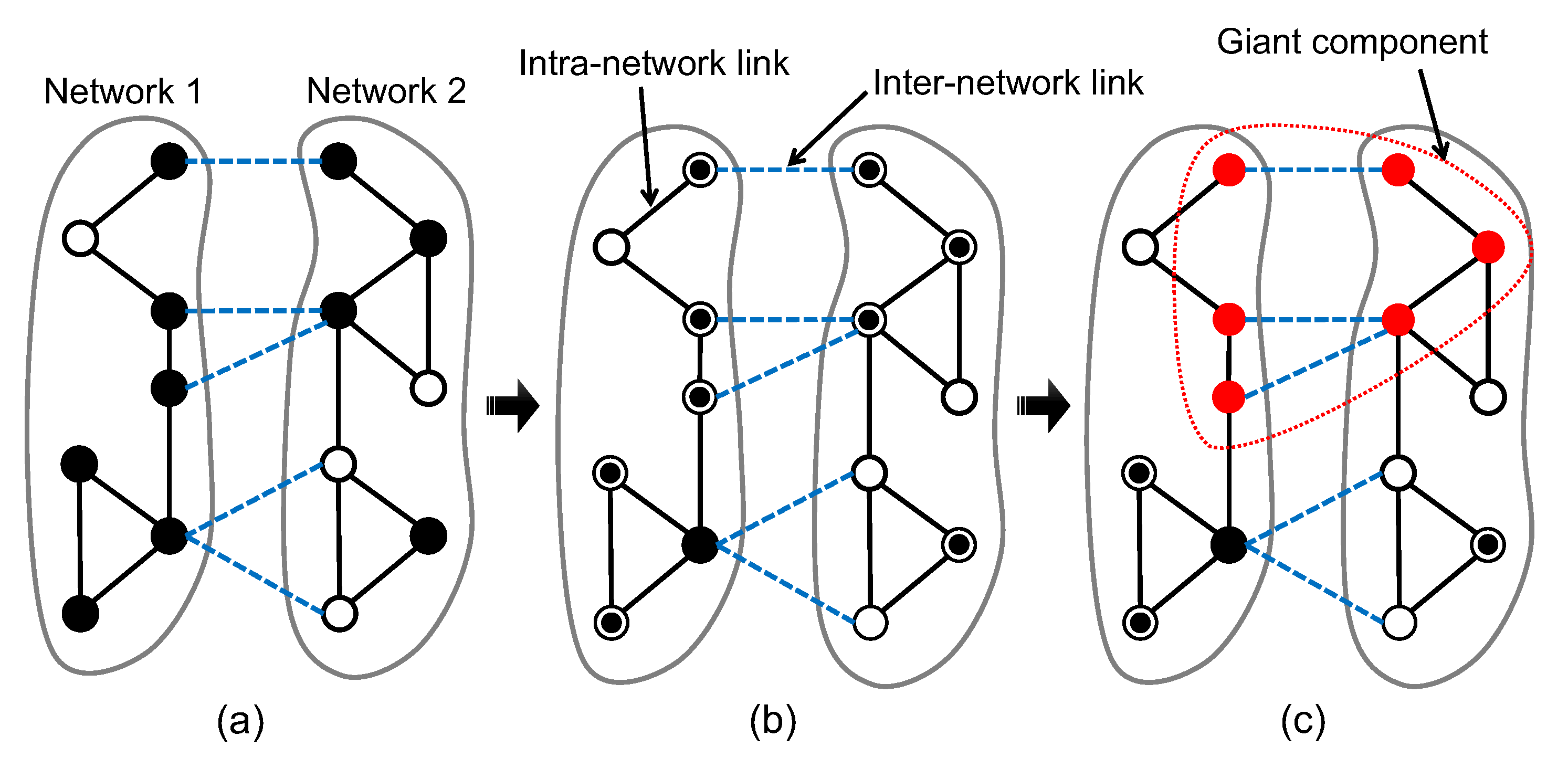
2.1. Network of Networks

2.1.1. Variables in NoN Models

The existing NoN model is characterized by modeling the node states to express the NoN availability. The state of an arbitrary node in the NoN is determined by those of its neighbors. A node can be in one of four states, each of which is characterized by three variables (

Table 1. Definition of network-of-networks (NoN) node states.

Symbol	Node State	${\mathit{n}}_{\mathit{i}}$	${\mathit{\sigma }}_{\mathit{i}}$	${\mathit{\rho }}_{\mathit{i}}$
	removed	0	0	0
	exists	1	0	0
	locally available	1	1	0
	globally available	1	1	1

), and state transitions occur in three steps (Figure 1). The variable $n_i$ indicates the existence of node i, and its value is predetermined as shown by Figure 1a. The value of ${\sigma }_i$, which expresses the local effectiveness of node i, is then determined based on the values $n_j$ of all nodes j that are connected via internetwork links, and shifts to the states shown in Figure 1b. ${\rho }_i$ is the global effectiveness of node i and is determined by whether the node is included in the giant component (GC) composed of locally effective nodes, which is shown in Figure 1c.

The B-NoN and C-NoN models define the local effectiveness ${\sigma }_i$ in the same way but the GC in different ways. This results in different definitions of the global effectiveness ${\rho }_i$, leading to a large difference in reliability between the two NoN models. In the following sections, we describe the definitions of ${\sigma }_i$ and ${\rho }_i$ in detail, along with the state-transition mechanisms shown in Figure 1.

2.1.2. Definition of Local Effectiveness

In a realistic NoN assumed by the B-NoN and C-NoN models, arbitrary nodes cannot be locally effective unless there is a node that is also locally effective in the interconnected network. For example, in brain functional networks, the function of “recognizing an image” can be achieved only by the cooperation of neural cells in two regions, namely, the posterior occipital cortex (vision) and the anterior cingulate cortex (recognition) [13]. In the same manner, an electric power supply system is realized by the cooperation of nodes in a power network and a control communication network [12]. As such, the NoN models express the local effectiveness of node i by defining the variable ${\sigma }_i$ as follows:

$${\sigma }_i=n_i[1-\prod _{j\in \mathcal{F}\left(i\right)}(1-n_i)],$$

(1)

where $\mathcal{F}\left(i\right)$ is the set of nodes connected to node i via internetwork links. For node i to be locally effective, Equation (1) requires (i) node i to exist and (ii) there to be at least one node connected to node i via internetwork links. If node i has no internetwork links, then the condition reduces to (i). For example, the node colored black in Figure 1b cannot become locally effective because both nodes connected via internetwork links are removed.

2.1.3. Definition of Global Effectiveness

The global effectiveness of a node is based on its connectivity to the GC consisting of locally effective nodes. The size of the GC is calculated using a method known as message passing, where a node (i) sends the probability of it being connected to the GC to all its adjacent nodes and (ii) updates this probability whenever the node receives the corresponding information from its neighboring nodes. A node can send information only when it is locally effective. At the beginning of message passing, the initial values of the probability are set to a random binary configuration of $\{0,1\}$, and the global effectiveness is determined by the converged value of the message passing process. The B-NoN and C-NoN models calculate the GC in different ways as explained in the following sections.

B-NoN Model

An image is recognized in the brain functional networks by the combination of the posterior occipital cortex, which is responsible for visual function, and the anterior cingulate cortex, which deals with recognition. These two regions compensate complementarily for the lack of information in each other; for instance, even if the posterior occipital cortex receives incomplete visual information from the eye, the anterior cingulate cortex can compensate for this lack and recognize the object. The B-NoN model reflects this as a logical OR-like dependence between the regions. A node is regarded as globally effective if either its adjacent nodes of the same network or those from other networks belong to the GC. For message passing in the B-NoN model, the variable ${\rho }_{i\to j}$ is defined as information sent from node i to node j within the same network and the variable ${\phi }_{i\to j}$ is defined as information sent from node i to node j of a different network:

$$\begin{array}{c}\hfill \begin{array}{c}\hfill {\rho }_{i\to j}={\sigma }_i[1-\prod _{k\in \mathcal{S}\left(i\right)\setminus j}(1-{\rho }_{k\to i})\prod _{l\in \mathcal{F}\left(i\right)}(1-{\phi }_{l\to i})],\\ \hfill {\phi }_{i\to j}={\sigma }_i[1-\prod _{k\in \mathcal{S}\left(i\right)}(1-{\rho }_{k\to i})\prod _{l\in \mathcal{F}\left(i\right)\setminus j}(1-{\phi }_{l\to i})],\end{array}\end{array}$$

(2)

where $\mathcal{S}\left(i\right)$ is the set of adjacent nodes of node i within the same network and $\mathcal{F}\left(i\right)$ is the set of adjacent nodes of node i from other networks. By this formulation, ${\rho }_{i\to j}$ and ${\phi }_{i\to j}$ become 1 if either ${\rho }_{k\to i}$ or ${\phi }_{l\to i}$ is 1, reflecting the logical OR-like dependence. Starting with random configurations of ${\rho }_{i\to j},{\phi }_{i\to j}\in \{0,1\}$, the global effectiveness ${\rho }_i$ as the converged probability of node i being connected to the GC through message passing is defined as

$${\rho }_i={\sigma }_i[1-\prod _{k\in \mathcal{S}\left(i\right)}(1-{\rho }_{k\to i})\prod _{l\in \mathcal{F}\left(i\right)}(1-{\phi }_{l\to i})].$$

(3)

C-NoN Model

In contrast to the B-NoN model, a node in the C-NoN model is globally effective if both its adjacent nodes of the same network and those from other networks belong to the GC. This model reflects the logical AND-like dependence that the power network and the control network are not mutually replaceable functions, whereas the functions in the inter-areal brain networks are complementary. Based on this characteristic, the variables ${\rho }_{i\to j}$ and ${\phi }_{i\to j}$ are defined as

$$\begin{array}{c}\hfill \begin{array}{c}\hfill {\rho }_{i\to j}={\sigma }_i\left[1-\prod _{k\in \mathcal{S}\left(i\right)\setminus j}(1-{\rho }_{k\to i})\right]\left[1-\prod _{l\in \mathcal{F}\left(i\right)}(1-{\phi }_{l\to i})\right],\\ \hfill {\phi }_{i\to j}={\sigma }_i\left[1-\prod _{k\in \mathcal{S}\left(i\right)}(1-{\rho }_{k\to i})\right]\left[1-\prod _{l\in \mathcal{F}\left(i\right)\setminus j}(1-{\phi }_{l\to i})\right].\end{array}\end{array}$$

(4)

In contrast to the formulation of the B-NoN model, ${\rho }_{i\to j}$ and ${\phi }_{i\to j}$ become 1 if both ${\rho }_{k\to i}$ and ${\phi }_{l\to i}$ are 1, reflecting the logical AND-like dependence. As the converged probability of node i being connected to the GC, the global effectiveness ${\rho }_i$ is then defined as

$${\rho }_i={\sigma }_i\left[1-\prod _{k\in \mathcal{S}\left(i\right)}(1-{\rho }_{k\to i})\right]\left[1-\prod _{l\in \mathcal{F}\left(i\right)}(1-{\phi }_{l\to i})\right].$$

(5)

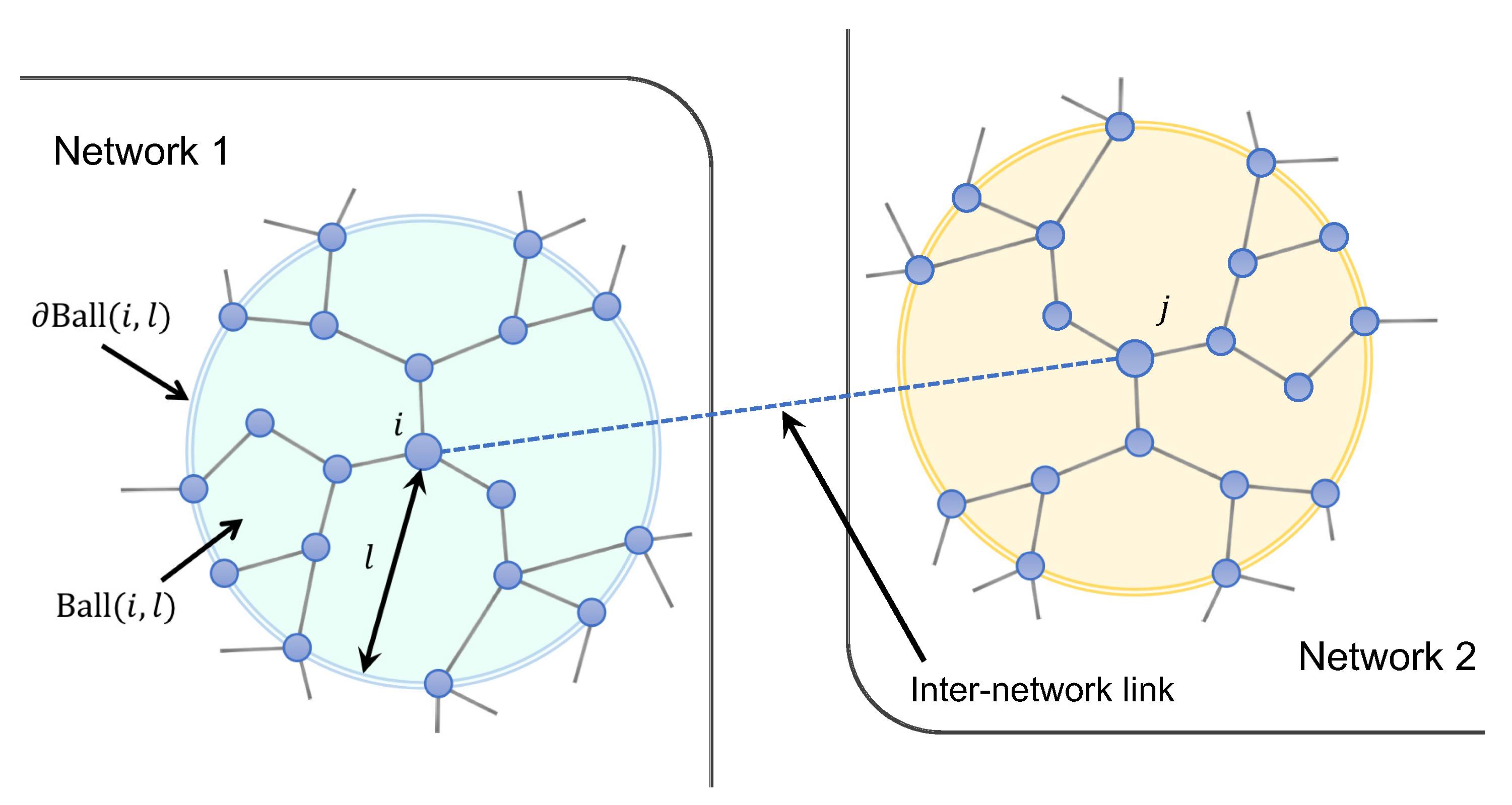
2.2. Influence Identification in a Network of Networks

The identification of highly influential nodes, which play important roles in robustness and diffusion, has been studied in many research domains, such as social networks [14,23], biology [24,25], marketing [26,27], and computer networks [16]. Because searching for the optimal influencers over a given network is an NP-hard problem [14], a number of heuristic methods have been proposed to date [28,29,30].

Herein, we also deal with influencer design to enhance NoN reliability, and therefore we focus on the recently proposed Collective Influence (CI) algorithm for influencer identification [31]. Not only does the CI algorithm outperform other existing methods in detecting influencers, it is also optimized for an NoN [13]. The influence on the network centered around node i is represented by ${\mathrm{CI}}_i$, which is defined as

$${\mathrm{CI}}_i=(k_i-1)\sum _{j\in \partial \mathrm{Ball}(i,l)}(k_j-1),$$

(6)

where $k_i$ is the degree of node i and $\partial \mathrm{Ball}(i,l)$ is the set of nodes located exactly l hops away from node i (Figure 2). ${\mathrm{CI}}_i$ is calculated as the product of the degree of node i and the sum of the degree of node j in $\partial \mathrm{Ball}(i,l)$. Furthermore, the definition of ${\mathrm{CI}}_i$ is expanded for an NoN as follows:

$$\begin{array}{ccc}\hfill {\mathrm{CI}}_i& =& (k_i^{intra}+k_i^{inter}-1)\sum _{j\in \partial \mathrm{Ball}(i,l)}(k_j^{intra}+k_j^{inter}-1)\hfill \\ & & +\sum _{j\in \mathcal{F}\left(i\right):k_j^{inter}=1}\left[(k_j^{intra}+k_j^{inter}-1)\sum _{m\in \partial \mathrm{Ball}(j,l)}(k_m^{intra}+k_m^{inter}-1)\right],\hfill \end{array}$$

(7)

where $k_i^{intra}$ and $k_i^{inter}$ are the degree of node i for intranetwork links and internetwork links, respectively. $\mathcal{F}\left(i\right)$ is the set of nodes connected to node i via internetwork links. The first term of Equation (7) corresponds to the CI of node i for Network 1 in Figure 2. The second term represents the sum of the CI of node j connected to node i via internetwork links, corresponding to Network 2 in Figure 2. The condition $k_j^{inter}=1$ indicates that node j is taken into account only if it has a single intermodular link. This is attributed to the NoN characteristic that the state of node j is not directly affected by node i if node j has more than one intermodular link according to Equation (1).

3. Network of Networks in Virtualized Networks

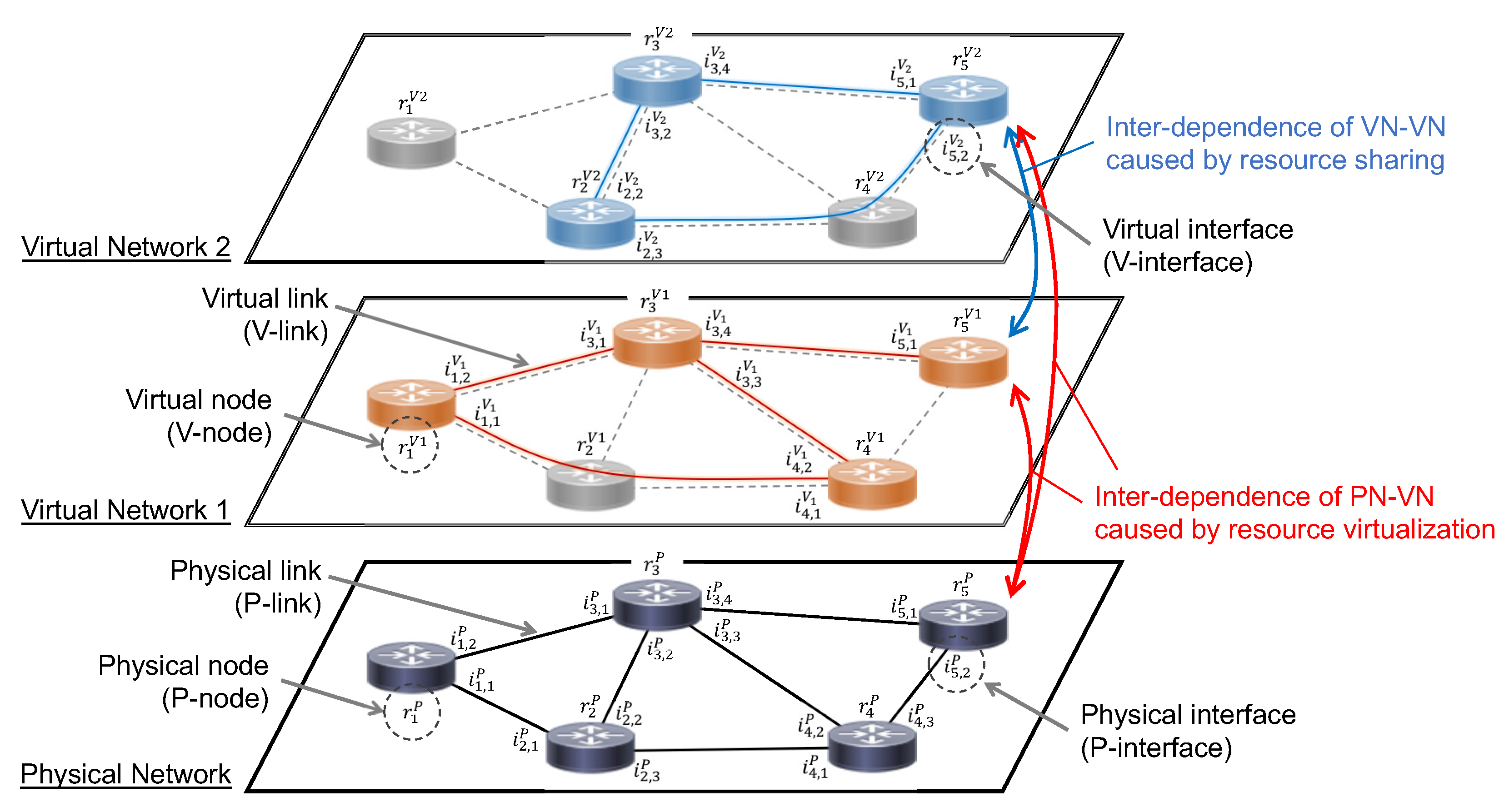
3.1. Interdependence of Virtualized Networks

In this study, we assume an interdependent layered network where a single PN is virtualized by network slicing, and multiple VNs are constructed on the PN as shown in Figure 3. A PN comprises physical nodes (P-nodes) and physical links (P-links). Similarly, virtual nodes (V-nodes) and virtual links (V-links) form a VN. Because of the virtualization of the PN, each V-node corresponds to exactly one P-node, while a V-link comprises multiple P-nodes and P-links that realize the shortest path connecting the two endpoint V-nodes. We assume that the connectivity structure of the PN is given by the infrastructure provider, whereas each VN realizes its own connectivity based on the requests of the service provider. In Figure 3, the P-node and V-node in VN k with common index i are represented as $r_i^P$ and $r_i^{V_k}$, respectively. The P-interface j of P-node i and the V-interface j of V-node i in VN k are represented as $i_{i,j}^P$ and $i_{i,j}^{V_k}$, respectively. Refer to

Table 2. List of variables used for the PV-NoN model and evaluation.

Variable	Value	Description	Equation
$n_i$	{0,1}	Existing state of node i	–
${\sigma }_i$	{0,1}	Local effectiveness of node i	Equation (1)
${\rho }_i$	{0,1}	Global effectiveness of node i	Equations (3) and (5)
${\rho }_{i\to j}$, ${\phi }_{i\to j}$	{0,1}	Probability information for message passing sent from node i to j	Equations (2) and (4)
${\mathrm{CI}}_i$	[0,∞]	Collective influence of node i	Equations (6) and (7)
$r_x^P$, $r_x^{V_k}$	–	Index for P-node x and V-node x on VN k	–
$i_{x,y}^P$, $i_{x,y}^{V_k}$	–	Index for P-interface y of $r_x^P$ and V-interface y of $r_x^{V_k}$	–
$B_{x,y}^P$	given	Buffer capacity for P-interface y of $r_x^P$	–
$n_{x,y}^P$	{0,1}	Availability state for P-interface y of $r_x^P$	–
$n_{x,y}^{V_k}\left(t\right)$	[0,∞]	Traffic state for V-interface y of $r_x^{V_k}$ at time t	–
$R_{x,y}^{V_k}\left(t\right)$	{0,1}	Vacancy state for V-interface y of $r_x^{V_k}$ at time t	Equations (8) and (10)
${\rho }_{x,y}^{V_k}\left(t\right)$	{0,1}	Traffic state for V-interface y of $r_x^{V_k}$ at time t	Equations (9), (11) and (12)
$\mathrm{CI}\left(r_x^P\right)$, $\mathrm{CI}\left(r_x^{V_k}\right)$	[0,∞]	Collective influence of $r_x^P$ and $r_x^{V_k}$	Equations (13)–(15)
$\eta$	[−1,1]	Assortativity for intra-network connectivity	Equation (17)
$\theta$	[−1,1]	Assortativity for inter-network connectivity	Equation (21)
$N^P$, $N^{V_k}$	given	Number of P-nodes and V-nodes on VN k	–
$L^P$, $L^{V_k}$	given	Number of P-links and V-links on VN k	–
W	given	Bandwidth for P-interfaces	–
$\lambda$	given	Arrival rate of packets	–
R	given	Number of packet re-transmission	–

for the description of the variables defined for the PV-NoN model and the evaluation in this paper.

Upon virtualization based on network slicing, the physical resources on the PN are shared among the VNs, thereby making the PN and VNs interdependent. Various services are being provided continuously over the VN, and environmental changes may occur at any instant because of traffic fluctuations. Consequently, our aim in this study is to model the VN availability under fluctuating traffic while considering the interdependence among the VNs caused by resource sharing. Although various physical resources on the P-nodes can be considered for virtualization (e.g., CPU, memory, storage, network I/O), we focus on the packet buffer memory (hereinafter referred to as the buffer) and network I/O because they are influenced directly by the traffic conditions. Consequently, we segment the P-nodes into physical interfaces (P-interfaces) and model the state of each P-interface taking the buffer and network I/O into consideration. The P-interface and the virtual interface (V-interface) are distinguished as shown in Figure 3.

Various approaches have been studied for partitioning physical resources, the aim being to improve the flexibility and efficiency of the virtualized networks [32,33,34]. Here, we assume three basic types of interface partitioning (

Table 3. Characteristics of three resource partitioning schemes for PV-NoN model.

	Type-SD	Type-UD	Type-DD
Interdependence of PN-VN	yes	yes	yes
Interdependence of VN-VN	no	yes	yes
Utilization guarantee	yes	no	yes
Utilization efficiency	no	yes	yes

). The most fundamental is type-SD (Statically Divided), in which resources (i.e., the buffer and network I/O) for the P-interface are divided statically for each VN; the upper limit of the number of packets stored and sent out from a V-interface is divided statically beforehand. With this type, constant performance is guaranteed for each VN and no traffic interference occurs, but the efficiency of resource utilization is not optimal. In contrast to type-SD, we also assume type-UD (UnDivided), in which the physical resource for each VN is not partitioned; the resource capacity for each VN is not guaranteed, and traffic in a VN could even occupy all the buffers and network I/O on the PN, but the physical resources can be utilized completely. As the third case, we assume type-DD (Dynamically Divided), in which the physical resources are allocated dynamically depending on the changing traffic conditions; the physical resources are not partitioned under normal conditions (as with type-UD), but they are partitioned when traffic congestion occurs. Therefore, type-DD allows physical resources to be used more efficiently while guaranteeing the resources for each VN. With all three types, resource virtualization makes the PN and VNs interdependent. Furthermore, with type-UD and type-DD, the sharing of physical resources among multiple VNs makes the latter interdependent.

3.2. Model of Network of Networks with Network Slicing

The PV-NoN model defines the availability state of interfaces to deal with traffic fluctuations and interdependence among a PN and VNs. Here, the word available denotes the state in which packets are transmitted at interfaces with no packet overflow. In the following sections, we describe the definitions of the input states of V-interfaces and P-interfaces and the availability states of V-interfaces calculated based on those input states.

3.2.1. Input States of Interfaces

In contrast to the existing NoN models, we introduce time in the form of the variable t because traffic conditions may change at any moment. The number of packets arriving at V-interface $i_{r,s}^{V_k}$ at time t is denoted as $n_{r,s}^{V_k}\left(t\right)$, which takes any positive value depending on the traffic conditions. The state of P-interface $i_{r,s}^P$ is expressed by the Boolean variable $n_{r,s}^P$, whose value is nominally 0 but becomes 1 if there is a malfunction and $i_{r,s}^P$ cannot send packets. The buffer capacity of $i_{r,s}^P$ is denoted as $B_{r,s}^P$.

3.2.2. Availability States of Interfaces

We define ${\sigma }_{r,s}^{V_k}\left(t\right)$ to express the availability state of $i_{r,s}^{V_k}$ considering the dependence among the PN and VNs. If $i_{r,s}^P$ has no malfunction and $i_{r,s}^{V_k}$ has no packet overflow, then $i_{r,s}^{V_k}$ is regarded as available and ${\sigma }_{r,s}^{V_k}\left(t\right)=1$ holds, otherwise ${\sigma }_{r,s}^{V_k}\left(t\right)=0$. However, the threshold for judging the presence of packet overflow differs among the three types of PV-NoN model as explained above, and details of their definitions are described below.

Type-SD

Because type-SD allocates the divided physical resources to each VN statically, there is no interdependence among the VNs. To derive the variable ${\sigma }_{r,s}^{V_k}\left(t\right)$ for $i_{r,s}^{V_k}$, we begin by defining a variable $R_{r,s}^{V_k}\left(t\right)$ that represents the presence of available capacity on $i_{r,s}^{V_k}$. ${\sigma }_{r,s}^{V_k}\left(t\right)$ for type-SD is then defined as follows using $R_{r,s}^{V_k}\left(t\right)$:

$$\begin{array}{ccc}\hfill R_{r,s}^{V_k}\left(t\right)& =& \left\{\begin{array}{cc}1\hfill & \mathrm{if}{\mathcal{B}}_{r,s}^P/N_{r,s}>n_{r,s}^{V_k}\left(t\right),\hfill \\ 0\hfill & \mathrm{otherwise},\hfill \end{array}\right.\hfill \end{array}$$

(8)

$$\begin{array}{ccc}\hfill {\sigma }_{r,s}^{V_k}\left(t\right)& =& R_{r,s}^{V_k}\left(t\right)\left(1-n_{r,s}^P\left(t\right)\right),\hfill \end{array}$$

(9)

where $N_{r,s}$ is the number of VNs that share $i_{r,s}^P$. $R_{r,s}^{V_k}\left(t\right)$ is defined so that it is 1 if the number of packets arriving at $i_{r,s}^{V_k}$ at time t does not exceed ${\mathcal{B}}_{r,s}^P/N_{r,s}$. Equation (9) defines the availability state of $i_{r,s}^{V_k}$ considering just VN k, which is in contrast to the other two types of PV-NoN model. By multiplying $R_{r,s}^{V_k}\left(t\right)$ and $\left(1-n_{r,s}^P\left(t\right)\right)$, ${\sigma }_{r,s}^{V_k}\left(t\right)$ is configured to be 1 only if the interface is available on both the virtual and physical levels.

Type-UD

The resources of the P-interface are undivided in the case of type-UD, and thus there is the interdependence that a traffic increase on a VN can limit the performance of the other VNs. That is, type-UD has logical AND-like interdependence whereby the performance can be guaranteed only when all VNs that are interdependent with each other are not congested, similar to the characteristics of the C-NoN model explained in Section 2. Here, in contrast to $R_{r,s}^{V_k}\left(t\right)$, we define $R_{r,s}^V\left(t\right)$ to express the presence of available capacity considering all VNs. Using $R^V$, the availability ${\sigma }_{r,s}^{V_k}\left(t\right)$ for type-UD is expressed as

$$\begin{array}{ccc}\hfill R_{r,s}^V\left(t\right)& =& \left\{\begin{array}{cc}1\hfill & \mathrm{if}{\mathcal{B}}_{r,s}^P>{\sum }_{l\in \mathcal{V}}{n}_{r,s}^{V_l}\left(t\right),\hfill \\ 0\hfill & \mathrm{otherwise},\hfill \end{array}\right.\hfill \end{array}$$

(10)

$$\begin{array}{ccc}\hfill {\sigma }_{r,s}^{V_k}\left(t\right)& =& R_{r,s}^V\left(t\right)\left(1-n_{r,s}^P\left(t\right)\right),\hfill \end{array}$$

(11)

where $\mathcal{V}$ is the set of all VNs. $R_{r,s}^V\left(t\right)$ is 1 if the number of packets arriving at $i_{r,s}^P$ at time t does not exceed ${\mathcal{B}}_{r,s}^P\left(t\right)$. This reflects the characteristic of type-UD that each V-interface considers the states of all interdependent V-interfaces, in contrast to type-SD. Because traffic fluctuations in one VN can influence all the other VNs, Equation (11) defines ${\sigma }_{r,s}^{V_k}\left(t\right)$ so that $i_{r,s}^{V_k}$ can be regarded as being available only if all interdependent V-interfaces have room for packets.

Type-DD

With type-DD, the resources of P-interfaces are reallocated among the VNs in a dynamic and complementary way depending on the traffic condition. This property allows type-DD to possess logical OR-like interdependence, which is seen in the B-NoN model described in Section 2: VN k can guarantee the performance if there is room in either VN k or the external VNs. Combining the characteristics of type-SD and type-UD, the availability of V-interfaces for type-DD is described as

$$\begin{array}{ccc}\hfill {\sigma }_{r,s}^{V_k}\left(t\right)& =& \left\{1-\left(1-R_{r,s}^{V_k}\left(t\right)\right)\left(1-R_{r,s}^V\left(t\right)\right)\right\}\left(1-n_{r,s}^P\left(t\right)\right).\hfill \end{array}$$

(12)

The first factor is 1 if the traffic condition satisfies either $R_{r,s}^{V_k}\left(t\right)=1$ or $R_{r,s}^V\left(t\right)=1$. This behavior expresses the logical OR-like interdependence that $i_{r,s}^{V_k}$ is available when either the allocated resources on VN k or the whole resources on the PN have room for packet processing.

3.3. Influencers in a Network of Networks with Network Slicing

In addition to modeling the availability state of an NoN with network virtualization, we aim to design NoN influencers to improve reliability. Consequently, we develop a method for detecting influencers in an NoN by applying the PV-NoN model based on the CI algorithm described in Section 2. As can be seen from the definition of the PV-NoN model described in the previous section, a failure of P-nodes occurring on the PN spreads to all interdependent VNs in any type of PV-NoN model. We therefore express the CI of P-node i as $\mathrm{CI}\left(r_i^P\right)$, and its definition is given based on Equation (7), corresponding to the sum of the influence on the PN centered around P-node i and the influence on each VN centered around V-node i. We define $\mathrm{CI}\left(r_i^P\right)$ as

$$\mathrm{CI}\left(r_i^P\right)=(k_i^P-1)\sum _{j\in \partial \mathrm{Ball}(r_i^P,l)}(k_j^P-1)+\sum _{k\in \mathcal{V}}\left[(k_i^{V_k}-1)\sum _{h\in \partial \mathrm{Ball}(r_i^{V_k},l)}(k_h^{V_k}-1)\right],$$

(13)

where $k_i^P$ and $k_i^{V_k}$ are the node degrees of $r_i^P$ and $r_i^{V_k}$, respectively. The definition of $\partial \mathrm{Ball}$ is the same as that described in Figure 2. The first term accounts for the CI of P-node i within the PN, and the second term accounts for the sum of the CIs of all the V-nodes that are interdependent with P-node i because of resource virtualization.

Regarding the CIs of the V-nodes, in the case of type-SD and type-DD, a specific V-node influences neither the V-nodes on the external VN nor the P-node on the PN, and thus $\mathrm{CI}\left(r_i^{V_k}\right)$ can be defined considering the influence on the VN to which the V-node belongs:

$$\mathrm{CI}\left(r_i^{V_k}\right)=(k_i^{V_k}-1)\sum _{j\in \partial \mathrm{Ball}(r_i^{V_k},l)}(k_j^{V_k}-1).$$

(14)

On the other hand, in the case of type-UD, it is possible for a V-node to occupy all of the resources shared among the VNs, and eventually the interdependent P-node runs out of capacity. Therefore, $\mathrm{CI}\left(r_i^{V_k}\right)$ can be defined as the sum of the CIs of all the interdependent V-nodes including the CI of the interdependent P-node as given by Equation (13):

$$\mathrm{CI}\left(r_i^{V_k}\right)=\mathrm{CI}\left(r_i^P\right)=(k_i^P-1)\sum _{j\in \partial \mathrm{Ball}(r_i^P,l)}(k_j^P-1)+\sum _{k\in \mathcal{V}}\left[(k_i^{V_k}-1)\sum _{h\in \partial \mathrm{Ball}(r_i^{V_k},l)}(k_h^{V_k}-1)\right].$$

(15)

4. Evaluation

In this section, we conduct simulation experiments that generate traffic over the VNs to evaluate the availability of the PV-NoN model. We begin by describing the methods for the evaluation, and then we explain the evaluation results.

4.1. Network Construction

This study assumes that an NoN comprises a PN and multiple VNs. The PN contains $N^P$ P-nodes and $E^P$ P-links, and similarly VN k contains $N^{V_k}$ V-nodes and $E^{V_k}$ V-links. If $N^P>N^{V_k}$, the VNs are mapped onto the PN so that the fewest P-nodes are shared among the VNs. The connectivity structure for the PN and VNs is determined based on a specific network model, for which we adopt the Erdös-Rényi (ER) model [35] and the Barabasi–Albert (BA) model [36], which generate node degrees following a Poisson distribution and a power-law distribution, respectively. Because it is virtually impossible to predict connectivity patterns in an IoT scenario with numerous types of services, we use the aforementioned models because they have been observed widely in actual networks and used for network evaluation to date [37,38,39,40]. Other types of network model are conceivable, such as the Watts–Strogatz (WS) model [41], the Waxman model [42], and the random geometric graph (RGG) model [43]. However, the Waxman model belongs to the class of random networks; in other words, it is a special case of the ER model. The degree distributions of the WS and RGG models are close to a uniform distribution, making it difficult to evaluate how network influencers and configuration affect assortativity. Furthermore, the WS model is characterized by its small-worldness, which the BA model shows as well.

Regarding the VN topologies, demands from service providers for connectivity reconfiguration now arise more frequently because of the flexibility and cost-efficiency of virtualized networks [10,34,44,45,46]. Therefore, this paper deals with the configuration of VN connectivity from the perspective of assortativity. Assortativity is a network metric for evaluating the correlation of node centrality in a given topology [17]. For example, looking at assortativity based on degree centrality, an assortative node is one whose connected neighbors have similarly high (or low) degrees, while a disassortative node is one that has either a high degree compared to its low-degree neighbors or vice versa. In this study, we configure the assortativity of a VN (intranetwork assortativity) and that among VNs (internetwork assortativity).

4.1.1. Intranetwork Assortativity

When node degree distribution is fixed on configuring topological connectivity within a network, the nodal degree is the only metric that can evaluate the centrality of the nodes. Consequently, we focus on the degree assortativity $\eta$ to configure the connectivity of a VN. We begin by introducing the remaining degree distribution $q\left(k\right)$, which is defined as

$$q\left(k\right)=\frac{(k+1)p(k+1)}{{\sum }_{j}jp\left(j\right)}.$$

(16)

The remaining degree distribution is related to the degree distribution $p\left(k\right)$ that describes the probability that the degree of a randomly chosen node corresponds to k. The remaining degree of a node in a path corresponds to the number of links of a node excluding the link it was arriving from. For a given $q\left(k\right)$, we can introduce the joint probability distribution $e(j,k)$, which indicates the probability that the two endpoints of a randomly chosen link have remaining degrees k and j. Consequently, the degree assortativity $\eta$ is defined as

$$\eta =\frac{1}{{\sigma }_q^2}[\sum _{j,k}jke(j,k)-(\sum _{j}jq\left(j\right){)}^2],$$

(17)

where ${\sigma }_q$ is the standard deviation of the remaining degree distribution $q\left(k\right)$. $\eta$ can take any value in the interval $[-1,1]$: $\eta >0$ and $\eta <0$ indicate an assortative network and a disassortative network, respectively, while $\eta =0$ indicates that the nodes are connected with each other randomly irrespective of their degrees. The degree distribution limits the range of feasible values of $\eta$.

Having constructed an initial VN topology with a specific degree distribution, we then set a target value of ${\eta }^{\prime }$ and rewire the links continuously [47,48] until the assortativity $\eta$ of the current topology approximates the given ${\eta }_{target}$. Note that we rewire a topology so that it is not split into submodules; if the generated VN topology is separated into more than one module, the former is reconstructed so that it is fully connected.

4.1.2. Internetwork Assortativity

As well as configuring the connectivity within each VN, we must also consider how to map the dependence of V-nodes because traffic fluctuation along the VNs causes interference. For example, we must investigate whether a V-node with high influence in one VN should be interdependent with a V-node of high influence in another VN. We therefore introduce the variable $\theta$ to evaluate the assortativity among VNs, and we configure the NoN structure from the perspective of mapping V-nodes on the VNs. Although we use the degree assortativity for connectivity within a VN because of its conditional limitation, we use the CI as a centrality measurement for the assortativity between networks, which is described in Section 2.

In a previous study [47], we developed a method for measuring the assortativity between networks to evaluate the interdependence of information networks. The assortativity of a set of links is represented as the sum of each link’s contribution to the assortativity of the entire network. Consequently, we begin by rewriting the definition of network assortativity described by Equation (17) as

$$\eta =\frac{1}{{\sigma }_q^2}\left(E\left[(J-U_q)(K-U_q)\right]\right),$$

(18)

where $U_q$ is the expected value of the remaining degree, and J and K are variables of the remaining degree that have the same expected value $U_q$. To expand the definition of assortativity for centrality metrics other than degree centrality, we introduce $p^{\prime }\left(c\right)$ as distribution of any kind of centrality metrics c on a VN. As for internetwork assortativity, the centrality of endpoint nodes of an internetwork link when the link is removed is equal to the centrality of those nodes on each VN topology. Hence, generalized assortativity ${\eta }^{\prime }$ can be defined based on degree assortativity $\eta$ in Equation (18) as follows:

$${\eta }^{\prime }=\frac{1}{{\sigma }_{p_j^{\prime }}{\sigma }_{p_k^{\prime }}}\left(E\left[(C_j-U_{p_j^{\prime }})(C_k-U_{p_k^{\prime }})\right]\right),$$

(19)

where $p_j^{\prime }$ denotes the centrality distribution on VN j. $U_{p_j^{\prime }}$ and ${\sigma }_{p_j^{\prime }}$ denote the expected value and the standard deviation of the centrality distribution $p_j^{\prime }$, respectively. $C_j$ denotes variables of the node centrality on VN j that have the same expected value $U_{p_j^{\prime }}$. Based on Equation (19), the contribution ${\theta }_l$ of link l to the assortativity ${\eta }^{\prime }$ of the entire network is defined as follows:

$${\theta }_l=\frac{(c_j-U_{p_j^{\prime }})(c_k-U_{p_k^{\prime }})}{{\sigma }_{p_j^{\prime }}{\sigma }_{p_k^{\prime }}},$$

(20)

where $c_j$ and $c_k$ are the node centrality of the two endpoints of link l. Finally, the internetwork assortativity $\theta$ (i.e., the assortativity of the set of links $L_{set}$ between two networks) is given by

$$\theta =\sum _{l\in L_{set}}{\theta }_l=\sum _{l\in L_{set}}\frac{(c_j-U_{p_j^{\prime }})(c_k-U_{p_k^{\prime }})}{{\sigma }_{p_j^{\prime }}{\sigma }_{p_k^{\prime }}}.$$

(21)

To map interdependent V-nodes among VNs, we begin by deploying the VNs randomly upon a PN. Then, similarly to the configuration of connectivity within a VN, we set a target value ${\theta }_{target}$ and repeatedly re-map until the $\theta$ calculated from the current VN interconnectivity approximates ${\theta }_{target}$ sufficiently.

4.2. Traffic Model

Network virtualization is expected to be used in a wide variety of situations and scales in the IoT scenario, resulting in unforeseeable traffic patterns [1,2,44,49,50]. Consequently, this study deals with a basic traffic model for performance evaluation, and the packet processing is designed on the basis of the $M/D/1/K$ queuing model [51]. The traffic condition changes discretely every time unit. Here, the average arrival rate (i.e., the rate at which a new packet is generated on a V-node at time t) is expressed by $\lambda$. The destination V-node of the generated packet is selected randomly from the other V-nodes on the VN to which the V-node belongs.

The routing path for a packet is determined so as to minimize the total number of P-links from the source V-node to the destination V-node. If there are multiple candidates for the shortest path, then one of them is selected randomly. For a pair of V-nodes, each path is determined statically and then left unchanged during the simulation. The total packet delay consists of the propagation delay and the queuing delay. A packet sent from a V-node at time t arrives at the next V-node at time $t+1$ because of the propagation delay (i.e., the propagation delay on each P-link is 1). Packets newly generated and packets arriving from neighbors at time t on a V-interface are stored on the buffer immediately. Because of the limitation of the bandwidth of P-links, the maximum number of packets that can be sent from one P-interface at time t is set uniformly to W, resulting in the queuing delay. Every P-interface holds a packet buffer that can store ${\mathcal{B}}_{r,s}^P$ packets, and packets waiting for their turn to be sent out are stored in the buffer. Packets are basically processed in a first in, first out (FIFO) manner, but the sending order is determined randomly when a V-interface receives multiple packets simultaneously. When a packet arrives at an intermediate full buffer (i.e., ${\sigma }_{r,s}^{V_k}\left(t\right)=0$), it is re-transmitted from its source V-node at the next time step. Packets are removed from the VN after either being re-transmitted R times or arriving at the destination V-node.

4.3. Evaluation Results

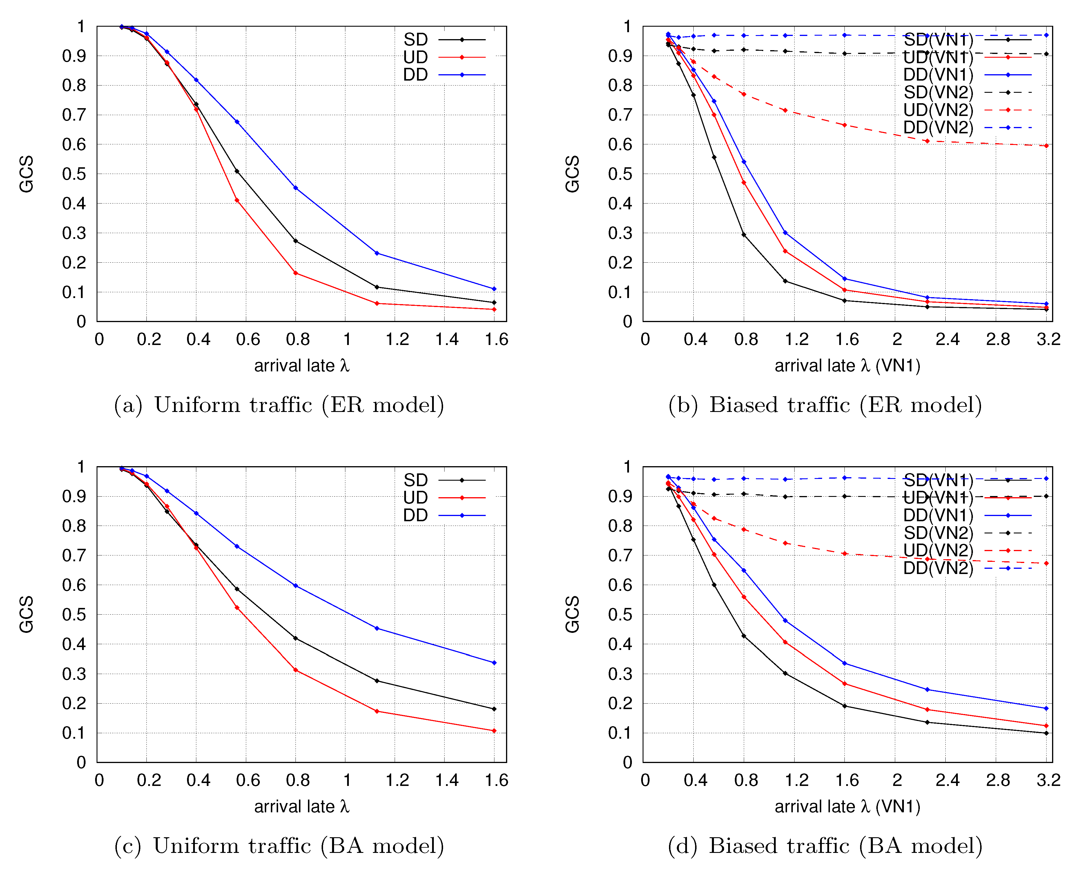
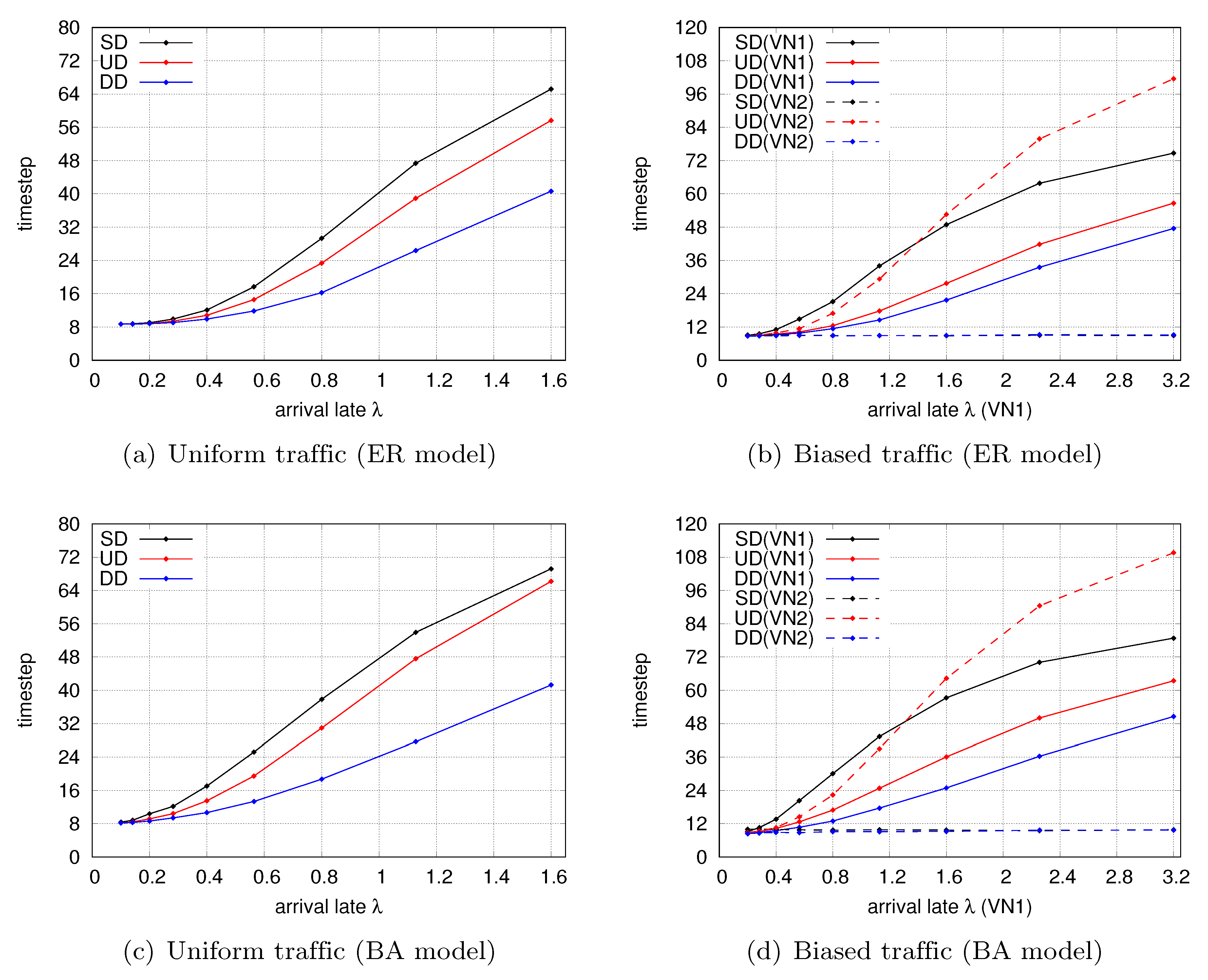
4.3.1. Comparing the Availability of the Three Types of PV-NoN Model

First, we compare the performance regarding the availability of the type-SD, type-UD, and type-DD versions of the PV-NoN model. We set $V=2$ as the number of VNs, $N^P=100$ and $N^{V_k}=0.9N^P(k\in \mathcal{V})$ for the number of nodes, and $L^P=3N^P$ and $L^{V_k}=3N^{V_k}(k\in \mathcal{V})$ for the number of links. The ER model is used to construct the PN topology, while both the ER and BA models are used for the VNs. In this evaluation, the inter/intranetwork connectivity is determined randomly without considering the assortativity. The packet buffer size for the P-interfaces is set to $\forall {\mathcal{B}}_{r,s}^P=20$, and the bandwidth for the P-interfaces is set to $W=1$; This means that each P-interface can send W packets from the network I/O every time unit, $\forall {\mathcal{B}}_{r,s}^P$ is determined assuming a TCP/IP environment, where in general packet size is set to 1.5 KB and buffer size is set to 8-256KB. We simulate two types of traffic conditions based on the arrival rate $\lambda$: (i) an equal amount of traffic flows on each VN and (ii) traffic is biased toward one of the two VNs. For (i), $\lambda$ for both VNs is changed in the range $[0.1,1.6]$, while for (ii) $\lambda$ is fixed at $0.2$ on VN1 and varied in the range $[0.2,3.2]$ on VN2.

We use the giant component size (GCS) and the packet delay as evaluation metrics to investigate NoN reliability from the perspectives of availability and communication performance. When a network topology is fixed, the evaluation on availability and communication performance is correlated with a given traffic fluctuation, i.e., availability increases when communication performance is high. However, when configuring a network topology, there can be a trade-off of availability and communication performance. If we configure a network topology to distribute the communication path, the network diameter can increase. This is the reason why we introduced communication performance in addition to availability as the evaluation metrics for evaluating reliability.

The GCS denotes the largest connected component on each VN consisting of available V-interfaces (i.e., ${\sigma }_{r,s}^{V_k}\left(t\right)=1$), which we use to evaluate the availability of the entire network for each VN. The GCS is often used as a metric for complex networks [31,37]. The packet delay denotes the average time required for a packet to be transmitted from its source to its destination, which is a more practical performance metric in communication networks. To see the impact of packet delay, we set the number of packet retransmissions to $R=100$. In a realistic TCP/IP implementation, a much smaller number of around 10 would be used for the number of retransmissions. However, with such small values, only those packets whose source and destination are near each other can be transmitted successfully and longer routes do not work on the VN, thereby making it difficult to evaluate the impact of packet delay appropriately. Instead, we used $R=100$ for the number of retransmissions. To evaluate the GCS, packets are created on the VN over 100 time steps and the GCS is measured at the 100th step, which is when the availability state of the V-interfaces is assumed to have converged and the simulation is finished. Regarding the packet delay, we create packets for the first 20 time steps and then continue the simulation until all the packets are either transmitted or removed from the VN. The packet delay is then counted for all the packets that were transmitted successfully during the simulation. Each result shown is the mean value from 50 simulations.

The simulation results for the GCS are shown in Figure 4. Each subfigure shows that type-DD gives the best availability of the three types of PV-NoN model. Although with type-SD traffic on one VN does not interfere with the other VN, neither VN can use its allocated physical resources fully because of the existence of the partition. Meanwhile, with type-UD the VNs can use their resources fully, but traffic between the VNs interferes with each other. Type-DD combines the characteristics of the other two types, thereby overcoming their shortcomings and improving the availability.

Another notable characteristic is observed in the simulation with biased traffic, as shown in Figure 4b,d. Because there is no resource partition among the VNs in type-UD, traffic congestion in one VN influences the other interdependent VNs in a cascading manner. Therefore, of the three dotted lines, only the red one drops as the arrival rate $\lambda$ increases. The extent to which cascades occur with type-UD is expected to increase further if the overlapping area of physical resources shared among the VNs increases. Meanwhile, even though type-DD also shares the physical resources of P-interfaces, the cascading of the performance degradation is prevented by the complementary dependence inspired by the B-NoN model.

Figure 5 shows the simulation results for the packet delay. The performance of the packet delay can basically be explained in correspondence with the GCS results, and we confirm that the delay is lowest with type-DD. Type-DD can be said to be superior to the other two types regarding practical performance as a communication network. Another notable point is that the type-SD packet-delay performance degrades when compared with the GCS results in Figure 4. No matter how large the buffer utilization (i.e., ${\sum }_{l\in \mathcal{V}}{n}_{r,s}^{V_l}\left(t\right)/{\mathcal{B}}_{r,s}^P$), the availability ${\sigma }_{r,s}^{V_k}\left(t\right)$, which is the basis of the GCS, is expressed as a binary state that does not take a negative value. On the other hand, the packet delay is expressed by taking any positive value reflecting the buffer utilization as it is. Based on these characteristics and results, we assume that interference among VNs with type-UD is likely to generate a number of moderately loaded V-interfaces to degrade the availability. Meanwhile, inefficient buffer allocation with type-SD is likely to generate rather few highly loaded V-interfaces to degrade the communication performance.

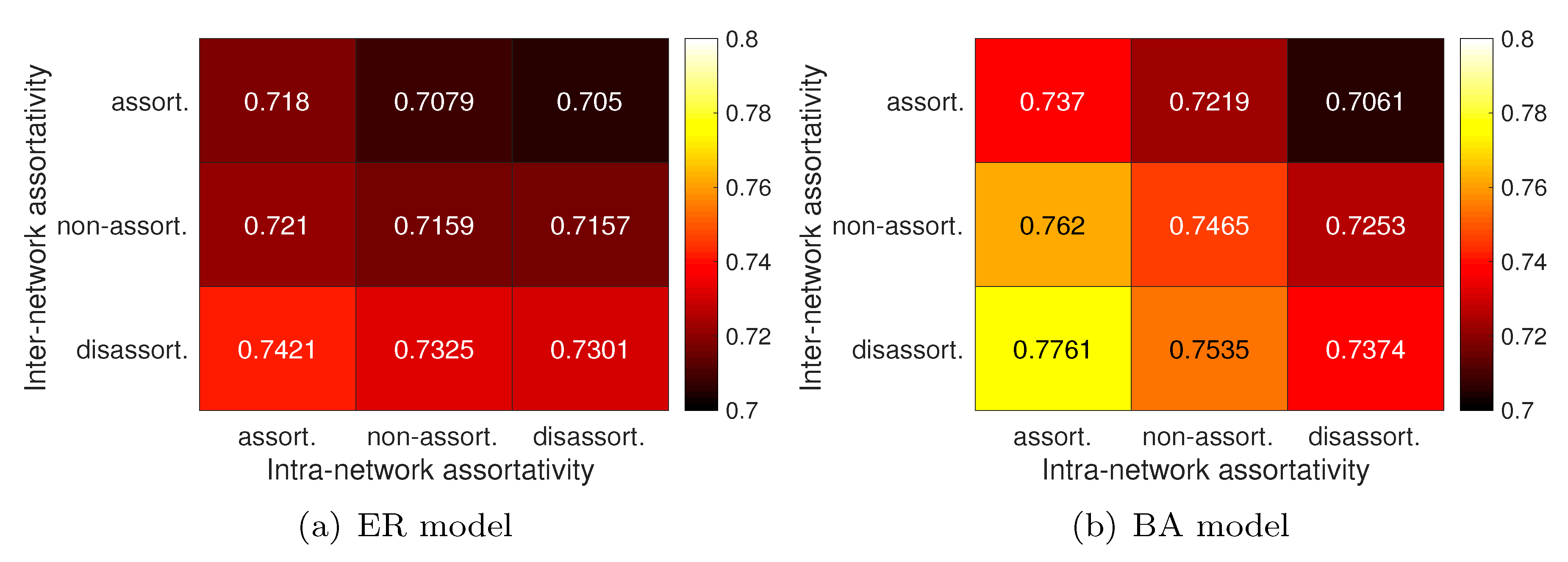
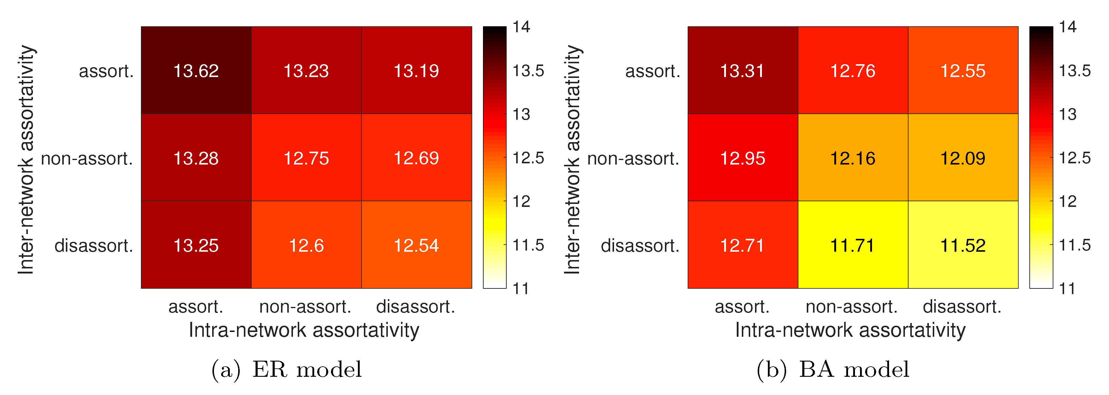
4.3.2. Designing Influencers on the PV-NoN Model

In this section, we investigate the importance of influencer deployment regarding inter/intranetwork assortativity. Because we confirmed above that type-DD prevails over the other two types, we focus on type-DD in this evaluation to investigate how to improve the performance further. The simulation settings are basically the same as those described in the previous evaluation, and we again use the GCS and packet delay to evaluate the availability and communication performance, respectively. However, to show the results concisely, we set the arrival rate for both VNs to $\lambda =0.5$ because the evaluation above confirmed that changes in performance can be seen with that value. As for the inter/intranetwork assortativity of network influencers, we picked three cases for each assortativity: (i) assort. is the case in which the rewiring procedure described in Section 4.1 is repeated until the connectivity converges with the highest assortativity, (ii) disassort. corresponds to the analogous case with the lowest assort. value, and (iii) non-assort. is the case in which the original connectivity pattern is maintained.

Figure 6 shows to the GCS evaluation results, and Figure 7 shows those for the packet delay. First, we find that the GCS is increased when the intranetwork connectivity is assortative (i.e., $\eta >0$) and the internetwork connectivity is disassortative (i.e., $\theta <0$). We have shown previously that an assortative single network is fragile against random failures [47]. However, it is notable that the results in Figure 7 tell us the opposite. We assume that when each VN topology is assortative, the overlapping of the shared physical resources among the VNs becomes concentrated on a local area of the entire NoN, thereby enhancing the availability when each VN is formed assortatively. By contrast, when $\theta <0$, the high-influence nodes are likely to not be shared among the VNs but rather to be dedicated to each VN. Consequently, an efficient resource utilization is realized, resulting in improved availability.

The results also show that the assortativity configuration has greater influence on networks based on the BA model. Because of the biased degree distribution and the limitation in the procedure of topology construction, influencers have greater impact with the BA model. However, because the ER model (i) has a more uniform degree distribution compared to the BA model and (ii) its topological structure is generated randomly, the impact of the assortativity configuration is smaller.

By contrast, Figure 7 shows that the packet-delay performance is increased when intranetwork connectivity is disassortative (i.e., $\eta <0$). When a network topology is formed assortatively, the network diameter becomes large and the communication performance degrades. It is true that assortative connectivity within each VN has a positive impact on availability, as seen in Figure 6. However, from a practical viewpoint of communication performance, we find that the increase of network diameter has a larger negative impact, resulting in degraded communication performance. As for the internetwork assortativity, the packet delay is decreased when it is disassortative, similar to the performance of GCS.

We ran simulations on type-UD and type-SD as well, but these merely confirmed that they show almost the same tendency in relation to the inter/intranetwork assortativity. A notable point is that the assortativity configuration had a larger influence on type-UD because the topological structure is closely related to the interference on the physical resources that is seen in type-UD.

5. Discussion and Conclusions

With the growing use of network slicing to implement the IoT network environment, it has been pointed out that traffic fluctuation in a sliced network could propagate to other networks [10,11]. It has therefore become necessary to consider reliable design for not just single networks and interconnected networks but also interdependent networks, i.e., NoN. The existing NoN models [12,13] describe the availability state of the NoN while considering the interdependence among the component networks, but are yet to be applied to practical systems of information networks. A contribution of the present work is that we considered layered VNs with network slicing as an NoN. We then proposed the PV-NoN model that expresses the availability state of an NoN that comprises a PN and VNs. The most notable aspect of our proposed model is that it considers traffic conditions and interdependence among the VNs. In this model, there are three types of interdependence according to the strategy used to divide the physical resources. With type-SD, the interface buffer on the physical nodes is divided statically. With type-UD, the buffer is undivided and the traffic among the VNs interferes with itself in a logical AND-like way, as seen in the C-NoN model. With type-DD, the buffer is usually undivided but is divided when there is congestion, in which case interference occurs in a logical OR-like way similarly to the B-NoN model.

To investigate a reliable NoN design in the assumed network virtualization environment, in our simulation experiments we measured the GCS and packet delay on an NoN to evaluate the availability and communication performance. In the first experiment, we compared the performance of the three types of PV-NoN model, and we confirmed that in every case type-DD achieves the highest availability and communication performance. This superiority of type-DD arises from combining the guaranteed resource utilization of type-SD and the utilization efficiency of type-UD. Furthermore, we confirmed that type-DD prevents the cascading of performance degradation even though it shares physical resources on P-interfaces similarly to type-UD. In that aspect, even when dealing with interdependent network systems other than those based on network slicing, there appears to be potential for improving the availability of the system by adopting the complementary dependence inspired by the B-NoN model. Regarding the application of brain functional networks, it is also the case that type-DD appears to be highly resilient to network failures, which is one of the most notable characteristics of brain networks [52,53].

We also conducted simulation experiments in which we configured the intra/internetwork assortativity of network influencers. The evaluation results confirmed that when the internetwork connectivity is disassortative (i.e., $\theta <0$), both the availability and communication performance are improved because influential nodes are not shared among the VNs, thereby avoiding interference among those nodes. When the intranetwork connectivity is assortative (i.e., $\theta >0$), the availability is improved while the communication performance is degraded. Although the internetwork connectivity affects only the interdependence among the VNs, the intranetwork connectivity also influences the structural performance of each VN in addition to the aforementioned interdependence. In detail, assortative connectivity within VNs localizes the area of physical resource sharing, thereby decreasing the interference among the VNs. At the same time, the assortative connectivity creates a long and narrow topology for each VN, thereby increasing the delay for packet communication. In a more practical scenario assuming the IoT environment, a larger-scale NoN must be considered, wherein the number of VNs or network components increases greatly. In that sense, optimizing the NoN’s structure would take an enormous amount of time and incur a huge computational cost. Consequently, structural configuration based on the assortativity of network influencers would help in designing reliable NoNs.

Because the main purpose of this paper was to deal with traffic fluctuations and interdependence on the assumed NoN environment, we configured the traffic pattern over the VNs in the simulation evaluation, which differentiates the performance among the three types of the PV-NoN model. However, it would also be valuable to investigate the influence of network failures occurring on the PN as a future task. Because of the rapid development of the IoT network environment, where a skyrocketing of network scale, traffic amount, and service variety is expected, various types of NoN systems are expected to emerge in the IoT scenario. Consequently, it is our opinion that the findings in this paper will help to solve upcoming issues related to other NoN systems in the IoT environment besides VN environments based on network slicing.

References

1. Arasteh, H.; Hosseinnezhad, V.; Loia, V.; Tommasetti, A.; Troisi, O.; Shafie-khah, M.; Siano, P. Iot-based smart cities: A survey. In Proceedings of the 2016 IEEE 16th International Conference on Environment and Electrical Engineering (EEEIC 2016), Florence, Italy, 7–12 June 2016; pp. 1–6. [Google Scholar]
2. Whitmore, A.; Agarwal, A.; Da Xu, L. The internet of things—A survey of topics and trends. Inform. Syst. Front. 2015, 17, 261–274. [Google Scholar] [CrossRef]
3. Gao, J.; Buldyrev, S.V.; Stanley, H.E.; Havlin, S. Networks formed from interdependent networks. Nat. Phys. 2011, 8. [Google Scholar] [CrossRef]
4. Zhou, X.; Li, R.; Chen, T.; Zhang, H. Network slicing as a service: Enabling enterprises’ own software-defined cellular networks. IEEE Commun. Mag. 2016, 54, 146–153. [Google Scholar] [CrossRef]
5. Zhang, H.; Liu, N.; Chu, X.; Long, K.; Aghvami, A.H.; Leung, V.C.M. Network slicing based 5G and future mobile networks: Mobility, resource management, and challenges. IEEE Commun. Mag. 2017, 55, 138–145. [Google Scholar] [CrossRef]
6. Michalopoulos, D.S.; Doll, M.; Sciancalepore, V.; Bega, D.; Schneider, P.; Rost, P. Network slicing via function decomposition and flexible network design. In Proceedings of the 2017 IEEE 28th Annual International Symposium on Personal, Indoor, and Mobile Radio Communications (PIMRC), Montreal, QC, Canada, 8–13 October 2017; pp. 1–6. [Google Scholar]
7. Yousaf, F.Z.; Gramaglia, M.; Friderikos, V.; Gajic, B.; von Hugo, D.; Sayadi, B.; Sciancalepore, V.; Crippa, M.R. Network slicing with flexible mobility and QoS/QoE support for 5G Networks. In Proceedings of the 2017 IEEE International Conference on Communications Workshops (ICC Workshops), Paris, France, 21–25 May 2017; pp. 1195–1201. [Google Scholar]
8. Rost, P.; Mannweiler, C.; Michalopoulos, D.S.; Sartori, C.; Sciancalepore, V.; Sastry, N.; Holland, O.; Tayade, S.; Han, B.; Bega, D.; et al. Network slicing to enable scalability and flexibility in 5G mobile networks. IEEE Commun. Mag. 2017, 55, 72–79. [Google Scholar] [CrossRef]
9. Li, X.; Casellas, R.; Landi, G.; de la Oliva, A.; Costa-Perez, X.; Garcia-Saavedra, A.; Deiss, T.; Cominardi, L.; Vilalta, R. 5G-crosshaul network slicing: Enabling multi-tenancy in mobile transport networks. IEEE Commun. Mag. 2017, 55, 128–137. [Google Scholar] [CrossRef]
10. Han, B.; Gopalakrishnan, V.; Ji, L.; Lee, S. Network function virtualization: Challenges and opportunities for innovations. IEEE Commun. Mag. 2015, 53, 90–97. [Google Scholar] [CrossRef]
11. Liu, J.; Jiang, Z.; Kato, N.; Akashi, O.; Takahara, A. Reliability evaluation for NFV deployment of future mobile broadband networks. IEEE Wirel. Commun. 2016, 23, 90–96. [Google Scholar] [CrossRef]
12. Buldyrev, S.V.; Parshani, R.; Paul, G.; Stanley, H.E.; Havlin, S. Catastrophic cascade of failures in interdependent networks. Nature 2010, 464, 1025–1028. [Google Scholar] [CrossRef] [Green Version]
13. Morone, F.; Roth, K.; Min, B.; Stanley, H.E.; Makse, H.A. Model of brain activation predicts the neural collective influence map of the brain. Proc. Natl. Acad. Sci. USA 2017, 114, 3849–3854. [Google Scholar] [CrossRef] [Green Version]
14. Kempe, D.; Kleinberg, J.; Tardos, É. Maximizing the spread of influence through a social network. In Proceedings of the 9th ACM SIGKDD International Conference on Knowledge Discovery and Data Mining, Washington, DC, USA, 24–27 August 2003; pp. 137–146. [Google Scholar]
15. Albert, R.; Jeong, H.; Barabási, A.L. Error and attack tolerance of complex networks. Nature 2000, 406, 378–382. [Google Scholar] [CrossRef] [PubMed] [Green Version]
16. Cohen, R.; Erez, K.; ben Avraham, D.; Havlin, S. Breakdown of the Internet under intentional attack. Phys. Rev. Lett. 2001, 86, 3682–3685. [Google Scholar] [CrossRef] [PubMed]
17. Newman, M.E.J. Assortative mixing in networks. Phys. Rev. Lett. 2002, 89, 208701. [Google Scholar] [CrossRef] [PubMed]
18. Wang, X.; Zhou, W.; Li, R.; Cao, J.; Lin, X. Improving robustness of interdependent networks by a new coupling strategy. Phys. A Stat. Mech. Appl. 2018, 492, 1075–1080. [Google Scholar] [CrossRef]
19. Dong, G.; Chen, Y.; Wang, F.; Du, R.; Tian, L.; Stanley, H.E. Robustness on interdependent networks with a multiple-to-multiple dependent relationship. Chaos Interdiscip. J. Nonlinear Sci. 2019, 29, 073107. [Google Scholar] [CrossRef] [PubMed] [Green Version]
20. Min, B.; Zheng, M. Correlated network of networks enhances robustness against catastrophic failures. PLoS ONE 2018, 13, e0195539. [Google Scholar] [CrossRef] [PubMed]
21. Cui, P.; Zhu, P.; Wang, K.; Xun, P.; Xia, Z. Enhancing robustness of interdependent network by adding connectivity and dependence links. Phys. A Stat. Mech. Appl. 2018, 497, 185–197. [Google Scholar] [CrossRef]
22. Shekhtman, L.M.; Danziger, M.M.; Vaknin, D.; Havlin, S. Robustness of spatial networks and networks of networks. Comptes Rendus Phys. 2018, 19, 233–243. [Google Scholar] [CrossRef] [Green Version]
23. Chen, W.; Wang, Y.; Yang, S. Efficient influence maximization in social networks. In Proceedings of the 15th ACM SIGKDD International Conference on Knowledge Discovery and Data Mining, KDD ’09, New York, NY, USA, 28 June–1 July 2009; pp. 199–208. [Google Scholar]
24. Chen, Y.; Paul, G.; Havlin, S.; Liljeros, F.; Stanley, H.E. Finding a better immunization strategy. Phys. Rev. Lett. 2008, 101, 058701. [Google Scholar] [CrossRef]
25. Newman, M.E.J. Spread of epidemic disease on networks. Phys. Rev. E. 2002, 66, 016128. [Google Scholar] [CrossRef] [Green Version]
26. Richardson, M.; Domingos, P. Mining knowledge-sharing sites for viral marketing. In Proceedings of the 8th ACM SIGKDD International Conference on Knowledge Discovery and Data Mining, Edmonton, AB, Canada, 23–26 July 2002; pp. 61–70. [Google Scholar]
27. Kiss, C.; Bichler, M. Identification of influencers–Measuring influence in customer networks. Decis. Support Syst. 2008, 46, 233–253. [Google Scholar] [CrossRef]
28. Kitsak, M.; Gallos, L.K.; Havlin, S.; Liljeros, F.; Muchnik, L.; Stanley, H.E.; Makse, H.A. Identification of influential spreaders in complex networks. Nat. Phys. 2010, 6, 888–893. [Google Scholar] [CrossRef] [Green Version]
29. Bao, Z.K.; Ma, C.; Xiang, B.B.; Zhang, H.F. Identification of influential nodes in complex networks: Method from spreading probability viewpoint. Phys. A Stat. Mech. Appl. 2017, 468, 391–397. [Google Scholar] [CrossRef]
30. Lü, L.; Chen, D.; Ren, X.L.; Zhang, Q.M.; Zhang, Y.C.; Zhou, T. Vital nodes identification in complex networks. Phys. Rep. 2016, 650, 1–63. [Google Scholar] [CrossRef] [Green Version]
31. Morone, F.; Makse, H.A. Influence maximization in complex networks through optimal percolation. Nature 2015, 524, 65. [Google Scholar] [CrossRef] [PubMed]
32. Wang, Z.; Wang, X.; Hou, F.; Luo, Y.; Wang, Z. Dynamic memory balancing for virtualization. ACM Trans. Archit. Code Optim. 2016, 13, 2:1–2:25. [Google Scholar] [CrossRef]
33. Beshley, M.; Romanchuk, V.; Chervenets, V.; Masiuk, A. Ensuring the quality of service flows in multiservice infrastructure based on network node virtualization. In Proceedings of the 2016 International Conference Radio Electronics Info Communications (UkrMiCo), Kiev, Ukraine, 11–16 September 2016; pp. 1–3. [Google Scholar]
34. Herrera, J.G.; Botero, J.F. Resource allocation in NFV: A comprehensive survey. IEEE Trans. Netw. Serv. Manag. 2016, 13, 518–532. [Google Scholar] [CrossRef]
35. Erdös, P.; Rényi, A. On random graphs, I. Publ. Math. (Debr.) 1959, 6, 290–297. [Google Scholar]
36. Barabási, A.L.; Albert, R. Emergence of scaling in random networks. Science 1999, 286, 509–512. [Google Scholar] [CrossRef] [PubMed]
37. Callaway, D.S.; Newman, M.E.J.; Strogatz, S.H.; Watts, D.J. Network robustness and fragility: Percolation on random graphs. Phys. Rev. Lett. 2000, 85, 5468–5471. [Google Scholar] [CrossRef] [PubMed]
38. Kawahigashi, H.; Terashima, Y.; Miyauchi, N.; Nakakawaji, T. Modeling ad hoc sensor networks using random graph theory. In Proceedings of the 2nd IEEE Consumer Communications and Networking Conference (CCNC 2005), Las Vegas, NV, USA, 6 January 2005; pp. 104–109. [Google Scholar]
39. Onat, F.A.; Stojmenovic, I. Generating random graphs for wireless actuator networks. In Proceedings of the 2007 IEEE International Symposium on a World of Wireless, Mobile and Multimedia Networks, Espoo, Finland, 18–21 June 2007; pp. 1–12. [Google Scholar]
40. Ding, L.; Guan, Z.H. Modeling wireless sensor networks using random graph theory. Phys. A Stat. Mech. Appl. 2008, 387, 3008–3016. [Google Scholar] [CrossRef]
41. Watts, D.J.; Strogatz, S.H. Collective dynamics of ‘small-world’ networks. Nature 1998, 393, 440. [Google Scholar] [CrossRef] [PubMed]
42. Waxman, B.M. Routing of multipoint connections. IEEE J. Sel. Area Commun. 1988, 6, 1617–1622. [Google Scholar] [CrossRef]
43. Dall, J.; Christensen, M. Random geometric graphs. Phys. Rev. E 2002, 66, 016121. [Google Scholar] [CrossRef]
44. Ochoa, S.F.; Fortino, G.; Fatta, G.D. Cyber-physical systems, internet of things and big data. Future Gener. Comput. Syst. 2017, 75, 82–84. [Google Scholar] [CrossRef]
45. Stankovic, J.A. Research directions for the internet of things. IEEE Internet Things J. 2014, 1, 3–9. [Google Scholar] [CrossRef]
46. Xu, L.D.; He, W.; Li, S. Internet of things in industries: A survey. IEEE Trans. Ind. Inform. 2014, 10, 2233–2243. [Google Scholar] [CrossRef]
47. Murakami, M.; Ishikura, S.; Kominami, D.; Shimokawa, T.; Murata, M. Robustness and efficiency in interconnected networks with changes in network assortativity. Appl. Netw. Sci. 2017, 2, 6. [Google Scholar] [CrossRef] [PubMed]
48. Van Mieghem, P.; Wang, H.; Ge, X.; Tang, S.; Kuipers, F.A. Influence of assortativity and degree-preserving rewiring on the spectra of networks. Eur. Phys. J. B 2010, 76, 643–652. [Google Scholar] [CrossRef] [Green Version]
49. Chang, Z.; Zhou, Z.; Zhou, S.; Chen, T.; Ristaniemi, T. Towards service-oriented 5G: virtualizing the networks for everything-as-a-service. IEEE Access 2018, 6, 1480–1489. [Google Scholar] [CrossRef]
50. Gupta, A.; Jha, R.K. A survey of 5G network: Architecture and emerging technologies. IEEE Access 2015, 3, 1206–1232. [Google Scholar] [CrossRef]
51. Kleinrock, L. Queueing Systems, Volume 2: Computer Applications; Wiley: New York, NY, USA, 1976; Volume 66. [Google Scholar]
52. Bullmore, E.; Sporns, O. The economy of brain network organization. Nat. Rev. Neurosci. 2012, 13, 336–349. [Google Scholar] [CrossRef] [PubMed]
53. Achard, S.; Salvador, R.; Whitcher, B.; Suckling, J.; Bullmore, E. A resilient, low-frequency, small-world human brain functional network with highly connected association cortical hubs. J. Neurosci. 2006, 26, 63–72. [Google Scholar] [CrossRef] [PubMed]
Figure 1. Example of state transition in Brain NoN (B-NoN) model [13]. The node symbols correspond to those defined in Table 1. The black lines indicate intranetwork links and the blue dashed lines indicate internetwork links.
Applsci 09 03809 g001
Figure 2. Expression of collective influence (CI). CI i is depicted in Network 1. Ball ( i , l ) is the area of influence of node i, and Ball ( i , l ) corresponds to the edge of Ball ( i , l ) . Networks 1 and 2 are interdependent via an internetwork link.
Applsci 09 03809 g002
Figure 3. Example of virtualized network based on network slicing.
Applsci 09 03809 g003
Figure 4. Variation of giant component size (GCS) with arrival rate λ . The vertical axis represents the GCS: 1 indicates that all the nodes on a VN are connected, whereas 0 indicates that they are completely disconnected. The solid lines in (a,c) correspond to the average GCS of the two VNs, whereas the GCS for each VN is plotted separately in (b,d). The horizontal axis represents the arrival rate λ . In (b,d), note that λ is changed on VN1 but fixed on VN2.
Applsci 09 03809 g004
Figure 5. Variation of packet delay with arrival rate λ . The vertical axis represents the packet delay, required time steps for a packet to be transmitted. Similarly to Figure 4, the solid lines in (a,c) correspond to the average packet delay of the two VNs, whereas the packet delays for each VN are plotted separately in (b,d). The horizontal axis represents the arrival rate λ . In (b,d), note that λ is changed on VN1 but fixed on VN2.
Applsci 09 03809 g005
Figure 6. GCS with changes in assortativity. The results are represented as heat maps. The GCS denotes the size of the largest connected component, and thus higher values indicate high performance (bright colors).
Applsci 09 03809 g006
Figure 7. Packet delay with changes in assortativity. Now, in contrast to the GCS, higher values indicate low performance (dark colors).
Applsci 09 03809 g007