A Method of Ontology Integration for Designing Intelligent Problem Solvers

Featured Application

In this paper, we present a method to integrate the knowledge-based systems based on ontology approach. Specially, this method can be used to design an integrated knowledge-based system for solving problems that involve the knowledge from multiple domains, such as Linear Algebra and Graph Theory. Given a specific problem that requires the knowledge from both domains, the system can reason upon the appropriate knowledge in the scope of the problem and generate a step-by-step solution which is very similar to that of humans. Therefore, this knowledge-based system can assist students in learning how to solve problems in many courses, thus meeting the requirements of an Intelligent Problem Solver in education.

Abstract

Nowadays, designing knowledge-based systems which involve knowledge from different domains requires deep research of methods and techniques for knowledge integration, and ontology integration has become the foundation for many recent knowledge integration methods. To meet the requirements of real-world applications, methods of ontology integration need to be studied and developed. In this paper, an ontology model used as the knowledge kernel is presented, consisting of concepts, relationships between concepts, and inference rules. Additionally, this kernel is also added to other knowledge, such as knowledge of operators and functions, to form an integrated knowledge-based system. The mechanism of this integration method works upon the integration of the knowledge components in the ontology structure. Besides this, problems and the reasoning method to solve them on the integrated knowledge domain are also studied. Many related problems in the integrated knowledge domain and the reasoning method for solving them are also studied. Such an integrated model can represent the real-world knowledge domain about operators and functions with high accuracy and effectiveness. The ontology model can also be applied to build knowledge bases for intelligent problem solvers (IPS) in many mathematical courses in college, such as linear algebra and graph theory. These IPSs have great potential in helping students perform better in those college courses.

1. Introduction

Nowadays, the knowledge from several sources needs to be integrated in order for machines to accomplish different tasks in a more intelligent way than conventional systems [1]. Knowledge integration is important in intelligent software development [2]. In order to achieve this, knowledge has to be processed and synthesized into knowledge bases. Many intelligent systems have introduced knowledge integration to increase their power.

Wolfram|Alpha is an engine for computing answers and providing knowledge [3]. The knowledge of this system is integrated from multiple knowledge domains, such as mathematics, science and technology, and society.

The IMS Learning Information Services is a tool to share data about learning [4]. This service supports the exchange of information about courses and learning outcomes between users. It is a combined knowledge-integrated system of learning management platforms, student record systems, and personnel systems.

Thus, knowledge integration is an imperative need for designing knowledge-based systems. Knowledge integration is the combination of multiple models for representing knowledge domains into a common model [1,5]. This integration has to meet some requirements, as follows:

• Practicality: The method for knowledge integration must be able to represent the real-world knowledge domain in a knowledge base, produce an inference engine that reasons upon the knowledge base, and solve practical problems via a similar reasoning process to that of humans;
• Accuracy: The components of the knowledge domain must be represented precisely and fully using the knowledge integration method, in a way that simulates human acquisition.

Ontology design and ontology integration are a potential approach to solve the problems of the integration of heterogeneous knowledge [6]. They provide sophisticated knowledge about the environment for task execution [7]. They allow the users to organize information on the taxonomies of concepts, with their own attributes, to describe relationships between the concepts. When data are represented by means of ontologies, software agents can better understand the content of the data and messages [8]. Domain-based knowledge can be modeled in ontology using ontology markup languages and various ontology tools, like Protege, OILed [9], PDDL (Planning Domain Definition Language) [10], and NDDL (New Domain Definition Language) [11].

The structure of an ontology consists of these basic components: concepts, relationships, and rules [12]. Concepts are the foundation for building the knowledge base, they make the representation clearer and more exact. Relationships on ontology perform connections between concepts. Inference rules are mechanisms for the reasoning to solve problems of the knowledge domain. The model for the integration of knowledge bases needs a knowledge kernel as ontology. Besides, solving a problem with the integrated model may require the knowledge of another pre-solved problem in the knowledge kernel. For example, in the knowledge domain of linear algebra, the knowledge of matrixes is the knowledge kernel. When solving a linear equations system, problems on the matrix, such as row transformation and column tranformation, have to be solved first [13]. Similarly, before solving a problem about vector spaces, it has to be converted to a matrix problem. Hence, the ontology-based model for integrating knowledge-based systems is a combination of the kernel ontology and other knowledge.

In this paper, an ontology model used as the knowledge kernel is presented. It includes concepts, relationships between concepts, and inference rules. Some problems for this kernel have been proposed and solved. This kernel is integrated with other knowledge, such as the knowledge of operators and functions, to form an integrated knowledge-based system. The integrating method works by integrating the knowledge components in the ontology structure. The problems in the integrated knowledge domain and the reasoning method to solve them are also studied. With such an integrated model, a real-world knowledge domain about operators and functions can be represented more accurately and effectively. These models are also applied to build the knowledge bases of intelligent problem solvers (IPS) in linear algebra and graph theory courses in university.

2. Related Works

There are various ontology-based methods for knowledge integration, most of which focus on basic kinds of ontology and are mainly used for information searching. They have not yet met the requirements of knowledge integration.

The Semanticscience Integrated Ontology (SIO) is an ontology for facilitating biomedical knowledge discovery [14]. SIO provides an ontological foundation for the Bio2RDF linked data for the life sciences project and is used for semantic integration and discovery for SADI-based semantic web services (Semantic Automated Discovery and Integration - SADI). However, the concepts of SIO are only basic information for searching.

Ontology-based knowledge integration is also used for semantic web services. Ontology WSMO is built based on the Web Service Modeling Framework (WSMO) [15]. WSMO defines four top level elements as the main concepts which have to be described in order to describe the semantic web services: ontologies, services, mediators, and goals. These methods only solve the integration of ontology as information but cannot support solving decision problems.

Fuzzy ontology integration is used for the representation of uncertain knowledge on the semantic web [16,17]. The author in [16] used description logic and fuzzy set theory to represent fuzzy logic and reason on it. The study in [17] presented a method to integrate fuzzy ontology based on consensus theory. Nonetheless, those methods are just theoretical and cannot be applied in the complex knowledge domains in practice.

Ontology COKB (Computational Objects Knowledge Base) is a useful ontology to represent complex knowledge domains [12]. This ontology can be used to describe many kinds of knowledge, such as knowledge about relationships, operators, and functions. It can be applied to build intelligent educational systems [18]. However, ontology COKB is too general to represent a specific knowledge domain, so it is very difficult to apply. Furthermore, the combination problems on the knowledge components in COKB have not yet been mentioned.

Ontology is also a technique model for information retrieval via the processing and translation of ontological knowledge into database search requests [19]. It is also used to compare the existing ontology-to-database transformation and mapping approaches in terms of loss of data, domain knowledge applicability, and structural mapping. Nonetheless, the mentioned knowledge in this study is simple, and the ontology integration has not yet been studied.

3. The Knowledge Kernel

3.1. Model of Knowledge Kernel

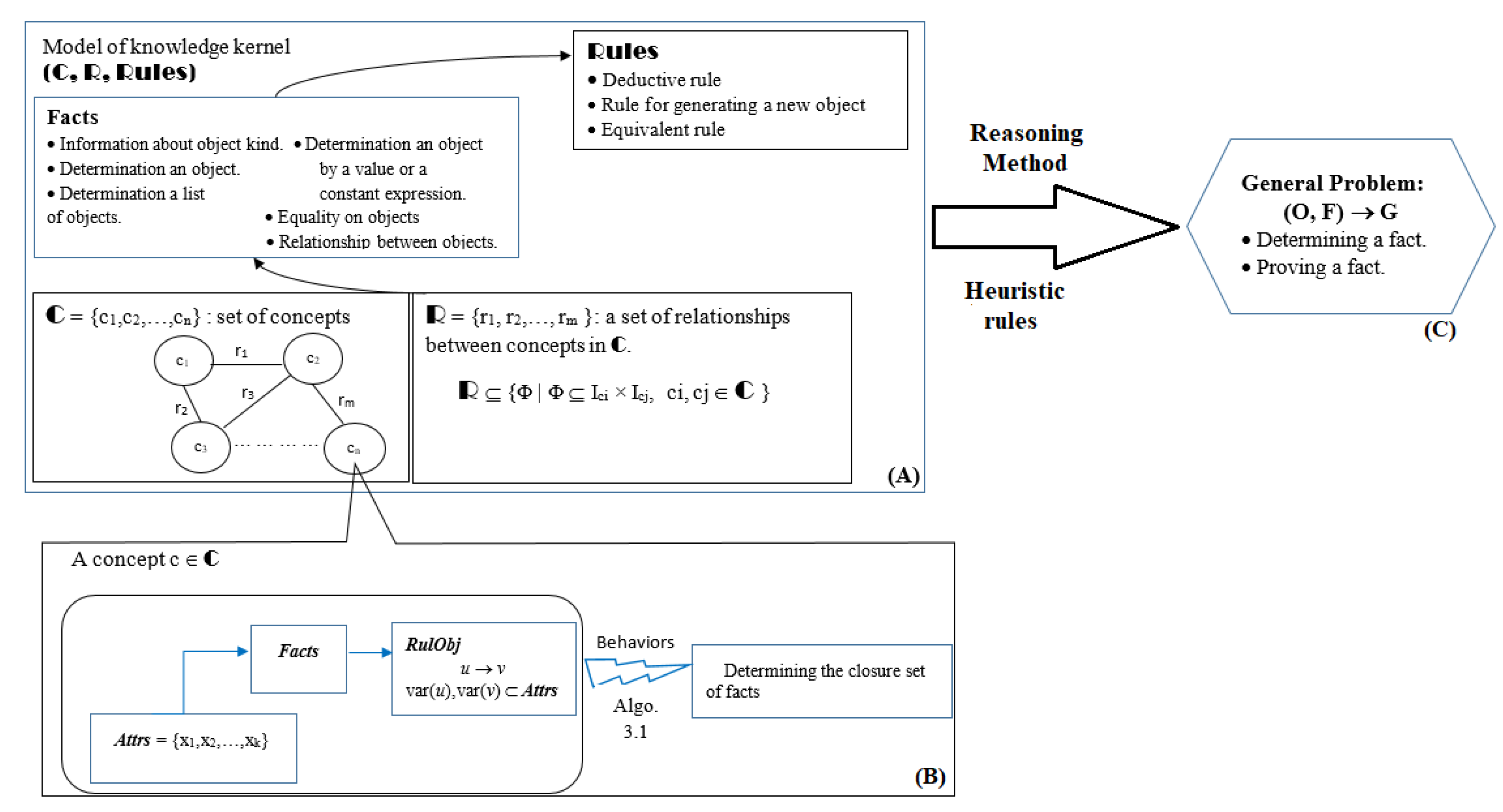
3.1.1. Structure of the Kernel

The model of the knowledge kernel in this paper was an ontology which was built based on the object-oriented approach. The model of the knowledge kernel was a tube:

(C, R, Rules),

in which C is a set of concepts, each concept is a class of objects, R is a set of binary relationships between concepts in C, and Rules is a set of inference rules.

Figure 1 shows the structure of the knowledge kernel. It is a tube (C, R, Rules) as part (A). The structure of each component is as

Table 1. Structure of components in the knowledge kernel.

C	R	Facts
- Each concept c ∈ C is a class of objects, it has an instance set Ic including objects.   • Fundamental concepts are the default concepts of the knowledge domain. A set of fundamental concepts is denoted: Co - Set C is a set of concepts, the structure of an object in a concept is a tube:   (Attrs, Facts, RulObj), in which:  ◊ Attrs is a set of attributes:   Attrs = AttrsVar ∪ AttrsList An attribute in AttrsVar is a variable which has the kind in Co:   AttrsVar ⊆ {x|x:c, c ∈ Co}. An attribute in AttrsList is a list of variables which have the same kind in Co:   AttrsList ⊆ {[x1, …, xn]|n ∈ and xi: c, c ∈ Co}. ◊ Facts is a set of facts on attributes in Attrs.   Facts ⊂ {f|f is a fact, var(f) ⊆ Attrs} ◊ RulObj is a set of deductive rules of the concept:   RulObj ⊂ {u → v|u ⊆ Attrs, v ⊆ Attrs, u ⊓ v = Ø}	R ⊂ {Φ|Φ ⊆ Ici × Icj,    ci, cj ∈ Co ∪ C,    ci ∈ C ∨ cj ∈ C} In the case of ci = cj, the properties of a relationship Φ are considered: reflexive, symmetric, asymmetric, and transitive.  * Relationships “is-a” < ∈ R:  Let c1, c2 ∈ C: c2 < c1 ⇔ c2 is a sub-concept of c1    $\iff \{\begin{array}{c}{c}_1.Attrs\subset c_2.Attrs\\ c_1.Facts⊑c_2.Facts\\ c_1.RulObj⊑c_2.RulObj\end{array}$	Classify kinds of facts: 1/Information about kind of object  Specification: x:c  Condition: x ∈ Σ*, c ∈ C 2/Determination an object  Specification: o  Condition: o ∈ Ic, c ∈ C 3/Determination of a list of objects  Specification: [o1, o2, …, on]  Condition: n ∈ , oi ∈ Ic,    c ∈ C (1 ≤ i ≤ n) 4/Determination of an object by a value or a constant expression  Specification: o = <const>  Condition: o ∈ Ic, c ∈ C <const>: constant 5/Equality on objects  Specification: x = y  Condition: x,y ∈ Ic, c ∈ C   or x = [x1, …, xn] and    y = [y1, …, yn] with xi, yi ∈ Ic, c ∈ C (1 ≤ i ≤ n) 6/Relationship between objects  Specification: x Φ y  Condition: Φ ∈ R,    x ∈ Icx, y ∈ Icy,    cx ∈ C, cy ∈ C * Kind(f): kind of fact f.

. Each concept in C is a class of objects. An object has attributes and internal relationships between them, it also has behaviors to solve the problems on it as part (B). This kernel had two kinds of problems: problems on an object and general problems (Section 3.2). The model of general problems is as part (C).

Definition 1.

Reference [20]: The closure of a set of facts

Let Obj = (Attrs, Facts, RulObj) be an object of concept in C, F be a set of facts.

The closure of a set of facts F by Obj, Obj.Closure(F), is a maximum extension of F by combining facts in F and Obj.Facts and reasoning on rules in Obj.RulObj.

3.1.2. Unification of Facts

Definition 2.

Given two facts f₁ and f₂. They are unified,≅, when they satisfy following conditions:

• f₁ and f₂ have them same kind of k;
• And if k = 1, 2, it means f₁ and f₂ are facts of information about object kind or determination of an object;

   Then f₁ = f₂;

  Or else if k = 3, it means f₁ and f₂ are facts of determination of a list of objects;

   Then NumberOfElements(f₁) = NumberOfElements(f₂);

      and f₁.o_i ≅ f₂.o_i ∀ i, 1 ≤ i ≤ NumberOfElements(f₁);

  Or else if k = 4, it means f₁ and f₂ are facts of determination of an object by a value or a constant expression;

   Then left(f₁) ≅ left(f₂) and compute(right(f₁)) = compute(right(f₂));

  Or else if k = 5: it means f₁ and f₂ are facts of equality on objects;

   Then (left(f₁) ≅ left(f₂) and right(f₁) ≅ right(f₂));

   Or (left(f₁) ≅ right(f₂) and right(f₁) ≅ left(f₂));

  Or else if k = 6, it means f₁ and f₂ are facts of relationships between objects;

   Then NameOfRelationship(f₁) ≡ NameOfRelationship(f₂) and

      Property(f₁) ≡ “symmetric” and (left(f₁) ≅ left(f₂) and right(f₁) ≅ right(f₂));

        or (left(f₁) ≅ right(f₂) and right(f₁) ≅ left(f₂));

    Or NameOfRelationship(f₁) ≡ NameOfRelationship(f₂);

     and (left(f₁) ≅ left(f₂) and right(f₁) ≅ right(f₂));

For which: • compute(expr): compute the value of the expression expr.

    • NameOfRelation(f): return the name of relation in fact f that is kind 6.

    • left(f), right(f): return the left side, right side of expression f.

Definition 3.

Reference [20]: Let x be a fact, A and B be sets of facts, the relationships between them have been defined as followed:

x ⊙ A ⇔ ∃ g ∈ A, x ≅ g    A ⊓ B = {x|x ⊙ A ∧ x ⊙ B}

A ⊑ B ⇔ ∀ x ∈ A, x ⊙ B    A ⊔ B = {x|x ⊙ A ∨ x ⊙ B}

A = B ⇔ A ⊑ B ∧ B ⊑ A    A\B = {x|x ⊙ A ∧ not(x ⊙ B)}

3.1.3. Rules—Set of Rules

A rule r ∈ Rules is one of three kinds, as follows:

• r is a deductive rule, it has the form u(r)→ v(r), where u(r), v(r) are sets of facts;
• r is a deductive rule for generating a new object, it has the form u(r)→ v(r), where u(r) and v(r) are sets of facts, they satisfy the conditions: ∃ object o, o ⊙ v(r) and not(o ⊙ u(r));
• r is an equivalent rule: h(r), u(r) ↔ v(r), where h(r), u(r) and v(r) are sets of facts, they satisfy the conditions: h(r), u(r)→ v(r), and h(r), v(r)→ u(r) are true.

3.2. Problems and Reasoning Methods on the Kernel Model

The kernel of knowledge model has two kinds problems: problems on an object and general problems with the kernel. Problems with an object relate to only the behaviors of an object. Each object of a concept in C uses its structure to solve the problems on itself. General problems with the kernel combine the knowledge of all objects and the kernel. When solving a general problem, the kernel has to apply the ability to solve problems with objects and the reasoning method on the knowledge of R and Rules.

3.2.1. Problem on an Object

An object of the Kernel Model has basic behaviors for solving problems on it. It is equipped abilities to solve problems such as: (i) Determine the closure of a set of attributes; (ii) Determine the closure of a set of facts; and (iii) Execute deduction and give solutions for problems. In this section, the algorithm for solving the problem (ii) is presented. The other problems can be solved by using this algorithm.

Algorithm 1. Determine the closure of a set of facts.
Input: Object Obj = (Attrs, Facts, RulObj), F is a set of facts related to Obj;
Output: Obj.Closure(F).
Step 0: Initialize variables   flag: = true;   KnownFacts: = F ⊔ Obj.Facts; Step 1. Classify the kinds of facts in KnownFacts; Step 2. Determine new facts from facts in   KnownFacts by using the reasoning rule; Step 3. Search the closure of facts of kind 2 in   KnownFacts; for fact2 in KnownFacts do;   if Kind(fact2) = 2 and fact2 ∈ C then # fact2 is a determined object;   KnownFacts: = KnownFacts ⊔ fact2. Attrs;   end if;  end do; Step 4. Search the closure of facts of kind 3 in   KnownFacts;  for fact3 in KnownFacts do;   if Kind(fact3) = 3; then for i from 1 to NumberfElements(fact3) do KnownFacts: = KnownFacts ⊔ fact3[i]; end if; end do;	Step 5. Search the rule r in Obj.RulObj which can be applied on KnownFacts;  while (flag! = false) do;   5.1. if (rule r can be found), then    for e in v(r) do;    KnownFacts: = KnownFacts ⊔ {e};    if (new facts can be determined), then    determine new facts from facts in KnownFacts by using deduce rules;    end if;    if Kind(e) = 2 and e ∈ C, then     KnownFacts: = KnownFacts ⊔       e.Closure(v(r));     if (new facts can be determined), then      determine new facts from facts in KnownFacts by using deduction rules;       end if;      end do; # for      end if; # 5.1    5.2. if (rule r cannot be found) then flag: = false;    end if; end do; # while Step 6. Obj.Closure(F): = KnownFacts.

Example 1.

In the knowledge domain about geometry, the triangle T is requested to give a solution for a problem {b, A, C}→ hb (hb is the length of altitude from the point B). The triangle T determines its closure of the set F = {b, A, C}. By Algorithm 1, the set T.Closure(F) is:

T.Closure(F) = {b, A, C, B, a, S, hb} by the following rules:

 r1: {A, C} → B by A + B + C = 180;

 r2: {A, B, b} → a, by Determine a/sin(A) = b/sin(B);

 r3: {a, b, C} → S, by S = a.b.sin(C)/2;

 r4: {S, b} → hb, by S = b.hb/2;

3.2.2. General Problem with the Model of the Kernel

The model of problems has the form: (O, F) → G, where O is the set of objects and F is the set of facts.

G = {“KEYWORD”: f} with “KEYWORD” may be the following:

-

Determine”: to determine the fact f;

-

Prove”: to prove the fact f.

The general algorithm for solving these problems was presented in [20]. It uses forward chaining reasoning for solving problems and applies heuristics rules as sample problems [21], arranging the priority to use inference rules. Each object attends the reasoning process by solving problems on itself as Algorithm 1.

4. Integration Between the Kernel and Other Knowledge

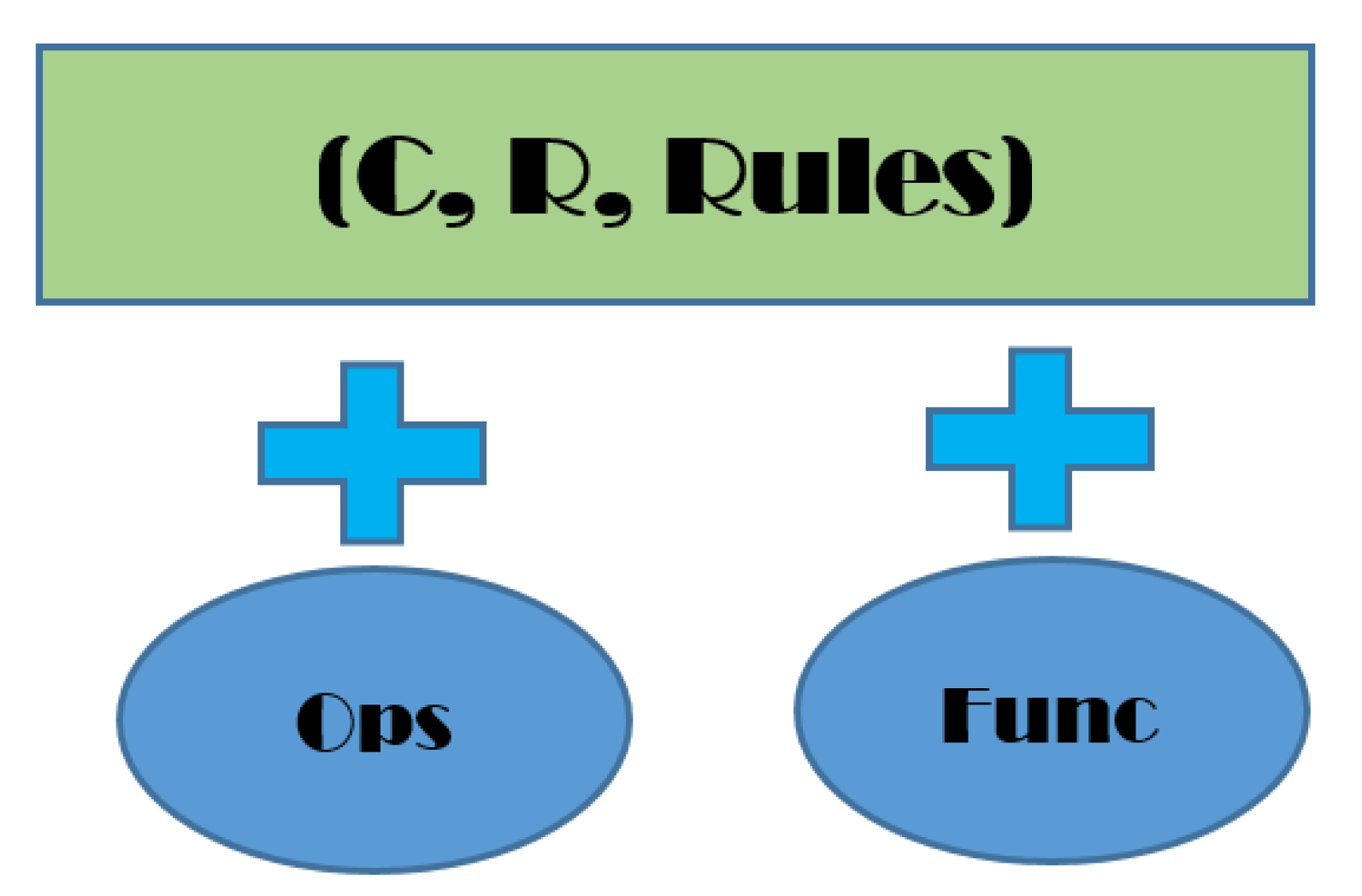
4.1. The Method to Integrate the Kernel and Other Knowledge

4.1.1. Knowledge Components of Operators and Functions

The knowledge of operators and functions is necessary to represent actual knowledge, especially the knowledge domains about computation. The knowledge of operators, called Ops-set, represents the computing operations over the objects in the knowledge domain. The knowledge of functions, called Funcs-set, represents how objects depend on each other, described as a set of conditions or a procedure over objects, in the knowledge domain. The integration of these components makes the knowledge base more powerful for representation and reasoning.

4.1.2. Principle to Integrate the Kernel and Components of Operators and Functions

The knowledge kernel can combine with other components, such as operators and functions, to represent real-world knowledge domains more accurately. When integrating new knowledge with the kernel (C, R, Rules), some aspects have to be considered:

• Building the structure of the additional component: This structure has to be built upon the kernel such that the integration of new concepts is seamless and consistent. Any additional component should have specification language similar to that of the kernel;
• Adding more kinds of facts: Facts in any additional component need to represent the real knowledge and connect with former kinds of facts in the kernel. This is a study about the unification of facts;
• Adding more kinds of rules from the additional component: More kinds of rules have been studied based on the integrated knowledge and need to be merged into the kernel;
• Proposing the problems with the reasoning by integrating the kernel knowledge and additional knowledge.

In this paper, we present a method to integrate the additional knowledge of operators and functions as Figure 2.

4.2. Integration with the Knowledge of Operators—Ops-set

4.2.1. Structure of the Ops-Set

Ops is a set of operators between concepts in C_o and C. Its structure is presented as

Table 2. Structure of the Ops-set.

Structure of the Ops-Set	Additional Facts	Additional Kind of Rules
Ops = O(1) ∪ O(2) In which:  + Set of unary operators O(1): O(1) ⊂ {⊕: Ici → Ick|ci, ck ∈ C}  + Set of binary operators O(2): O(2) ⊂ {⊗: Ici × Icj → Ick|      ci, cj, ck ∈ C}  Each operator is checked for its properties: commutation, association, identity.	Op.1. Dependence of an object by an expression.  Specification: x = <expr>  Condition: x ∈ Ic, c ∈ C   <expr>: expression Op.2. Equality of expressions Specification:    <expr1> = <expr2> Condition: <expr1>: expression    <expr2>: expression	r is an equation rule, it has the form:    g = h where g, h are expressions of objects. Denote:   left(r) = g   right(r) = h

:

An operator in the Ops-set is specified as below:

Operator-def: = OPERATOR <name>

ARGUMENT: argument-def+

RETURN: return-def+;

PROPERTY: prob-type+

[constraint]

[variables]

[statements]

END OPERATOR.

argument-def: = <name>: type

return-def: = name: type

prob-type: = commutative|associative|identity

statement: = name: = <expression>.

4.2.2. Problems and Reasoning Methods on the Knowledge of Operators

The model of problems has the form (O, F, E) → G [22], where O is the set of objects, F is the set of facts, E = {e₁, e₂,…, e_k} is the set of equations, and G is:

G = {“KEYWORD”: f} with “KEYWORD” is a keyword of the goal and f is a fact. Besides keywords as Section 3.2.2, “KEYWORD” may be as follows:

-

Compute”: to determine the value of f when f is an expression;

-

Transform”: transform an object into an expression between certain objects.

Algorithm2. Given a knowledge domain combining with operators K = (C, R, Rules) + Ops, and a problem P = (O, F, E) → G on this knowledge domain. This algorithm will solve the problem P though the following steps:
Input: The problem P = (O, F, E) → G
Output: The solution of the problem P.
The idea of the algorithm: Using objects in O, it determines the closure of each object by Algorithm 1. After that, it solves the problem (O, F) → G on the knowledge kernel. Secondly, it uses the knowledge of operators, which was integrated, to process the equations in E for getting new facts. Some new objects may be generated in this reasoning. If the goal G is achieved at any time, this algorithm will stop.
Step 0: Initialize variables;  flag: = true;  KnownFacts: = F ⊔ E;  Sol: = [ ]; # solution of problem; Step 1. Record elements in hypothesis and goal;  Classify kinds of facts in F and E. Step 2. Check G;  If G is obtained, then go to step 6. Step 3: Use objects in set O and the set of facts in F and E to determine the closure of each object by Algorithm 1; Step 4: Use the equations in E to generate the new facts as relationship form;  Use the relationships in F to generate the equations;  Update KnownFacts and Sol. Step 5: Select a rule in the set Rules for producing new facts or new objects; While (flag! = false) and not (G is determined) do  Search r in the Rules set, which can be applied to KnownFacts. 5.1. Case: r is an equation rule;  if (r has form: g = h), then:   r can generate a set of new facts. A: = r(KnownFacts) = {f|Kind(f) = 2 ∨    Kind(f) = 3 ∨ Kind(f) = Op.1 ∨    Kind(f) = Op.2}   s: = [r, KnownFacts, A];   Sol: = [op(Sol), s];	if (r generates a new object o) and not (o ⊙ KnownFacts), then:  KnownFacts: = KnownFacts ⊔ A;  Go to Step 3 with new object o; Or else:  KnownFacts: = KnownFacts ⊔ A; continue; end if; end if; #5.1 5.2. Case: r has another kind;  Transform equations in E to relationships between objects if possible;  Update KnownFacts and Sol;  Solve the problem (O, KnownFacts) → G based on the knowledge of the kernel (C, R, Rules) by algorithms in Section 3.2;  end if; #5.2 Step 6: Conclusion of the problem;  If G is determined, then:  Problem (O, F, E) → G is solvable;  Sol is a solution of the problem;  Reduce the solution found by excluding redundant rules and information in the solution;  Or else   Problem (O, F, E) → G is unsolvable;  end if;

Example 2.

In the knowledge domain about direct current electrical circuits,Ops is the set of the knowledge of operators being series connection (+) and parallel connection (//) between two circuits. We considered the problem as follows:

Problem P1: Three resistors are connected like the Figure 3. Resistor T1 has value 45 Ω, Resistor T3 has value 90 Ω. The total current is 0.5 A, current though T3 is 0.3 A.

What is the current thought T1?

+ Model of problem:

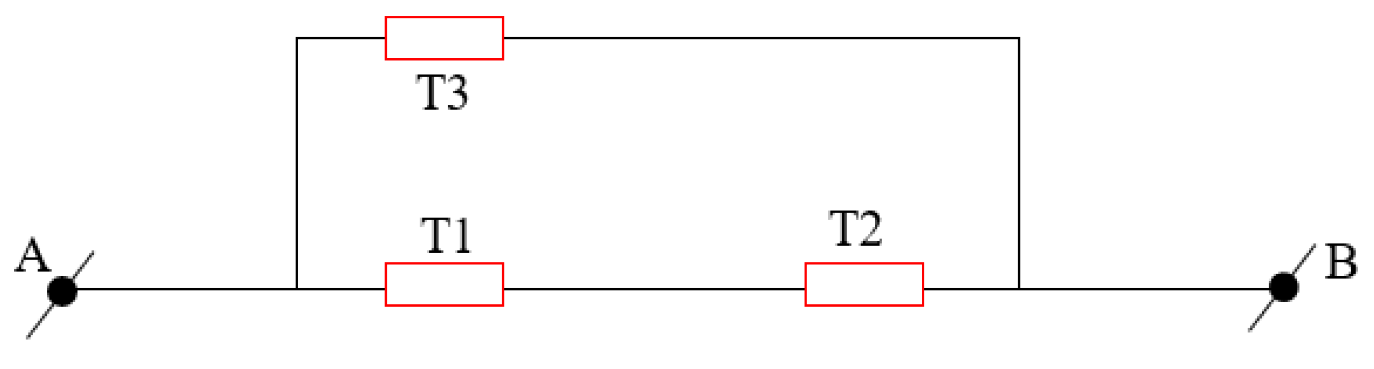
O: = {T1, T2, T3: RESISTOR; AB: CIRCUIT}

F: = {AB = T1 + T2//T3, T1.R = 45, T3.R = 90, T3.I = 0.3, AB.I = 0.5}

G: = {T1.I}.

+ Searching rules of Algorithm 2:

 S1: {T1 + T2//T3 = (T1 + T2)//T3} by rule: ”equation rule”;

 S2: {Let [CD, CIRCUIT], CD = T1 + T2}, by rule: ”rule for generating a new object”;

 S3: {AB = T1 + T2//T3, T1 + T2//T3 = (T1 + T2)//T3, CD = T1 + T2} → {AB = CD//T3},

   by rule: ”deductive rule”;

 S4: {AB = CD//T3} → {CD.I = CD.I + T3.I}, by rule: “deductive rule of parallel circuits”;

 S5: {CD = T1 + T2} → {CD.I = T1.I}, by rule: “deductive rule of series circuits”;

 S6: {T3.I = 0.3, AB.I = 0.5, AB.I = CD.I + T3.I} → {CD.I = 0.2}, by rule: “ equation rule for solving”;

 S7: {CD.I = 0.1, CD.I = T1.I} → {T1.I = 0.2}, by rule: “equation rule for solving an equation”.

4.3. Integration with the Knowledge of Functions—Funcs-set

4.3.1. Structure of the Funcs-Set

Funcs is a set of functions in the knowledge domain. The structure of the Funcs-set, some additional facts, and additional kinds of rules about functions are shown in

Table 3. Structure of the Funcs-set

Structure of the Funcs-Set	Additional Facts	Additional Kinds of Rules
Let F = {f|f is a function}:  α: F → N: assigning the number of arguments to a function. Funcs ⊆ {f ∈ F|n = αK(f),   f: Ic1 × Ic1 … × Icn → Ic,    c1, c2,…, cn, c ∈ C}. Each function is checked for its properties: commutation.	Fu.1. Determination of a function.  Specification: f(x1, x2, …, xn);  Condition: f ∈ Funcs, n = α(f),   f: Ic1 × Ic2 ×…× Icn → Ic,   xk ∈ Ick, ck ∈ C (1 ≤ k ≤ n). Fu.2. Dependence of an object on a function.  Specification: o = f(x1, x2, …, xn);  Condition: f ∈ Funcs, n = α(f),    f: Ic1 × Ic2 ×…× Icn → Ic,    xk ∈ Ick, ck ∈ C (1 ≤ k ≤ n),    o ∈ Ic, c ∈ C. Fu.3. Dependence of a function on an expression.  Specification:    f(x1, x2, …, xn) = <expr>.  Condition: f ∈ Funcs, n = α(f),     f: Ic1 × Ic2 ×…× Icn → Ic,    xk ∈ Ick, ck ∈ C (1 ≤ k ≤ n), c ∈ C,     <expr>: expression. Fu.4. Relationship between functions. Specification:   f(x1, x2, …, xn) Φ g(y1, y2, …, ym). Condition: Φ ∈ R, f ∈ Funcs,       g ∈ Funcs,    n = α(f), m = α(g); c, c’ ∈ C;    f: Ic1 × Ic2…× Icn → Ic,    xk ∈ Ick, ck ∈ C (1 ≤ k ≤ n),    g: Ib1 × Ib2…× Ibm → Ic’,    yk ∈ Ibk, bk ∈ C (1 ≤ k ≤ m).	r is an equation rule, it has the form: f = g, where f, g are functions or expressions. Denote:   left(r) = f   right(r) = g

.

A function in the Funcs-set is specified as followed:

function-def: = FUNCTION name;

ARGUMENT: argument-def+

RETURN: return-def;

[constraint];

[facts];

[variables];

[statements];

ENDFUNCTION;

statements: = statement-def+;

statement-def: = assign-stmt|if-stmt|for-stmt;

asign-stmt: = name: = expr;

if-stmt: = IF logic-expr THEN statements+ ENDIF;

|IF logic-expr THEN statements+ ELSE statements+ ENDIF;

for-stmt: = FOR name IN [range] DO statements+ ENDFOR;

4.3.2. Problems and Reasoning Methods on the Knowledge of Functions

When integrating the knowledge of functions, the general problem of the integration has the form (O, F) → G, as in Section 3.2, in which the set of facts F includes the additional facts as function-kinds Fu.1, Fu.2, Fu.3, and the set G is modeled as:

G = {“KEYWORD”: f} with “KEYWORD” is a keyword of the goal and f is a fact, “KEYWORD” may be the followings:

-

Compute”: to determine the value of f when f is a function;

-

Prove”: prove the fact f.

Algorithm 3. Compute the value of a function.
Give a knowledge domain combining functions K = (C, R, Rules) + Funcs, and a problem P = (O, F) → G on this knowledge domain, with G = {“Compute”: g(x1, x2, …, xn)}, where g is a function and xk are objects (k = 1 … n).
Input: The problem P = (O, F) → G
G = {“Compute”: g(x1, x2, …, xn)} with: g: Ic1 × Ic2 … × Icn → Ic
xk ∈ Ick, ck ∈ C (1 ≤ k ≤ n), c ∈ C
Output: The value of g(x1, x2, …, xn).
The idea of the algorithm: The set F is split into two sets: F1—the set of facts in the knowledge kernel, F2—the set of facts about functions. Firstly, using the knowledge kernel, the algorithm uses the objects and facts in the hypothesis (O, F1) to determine new facts by applying the sub-algorithm for solving problems on the kernel model, as in Section 3.2.2. Secondly, combining with the facts in the set F2, the algorithm uses the integrated knowledge of functions to compute the value of g.
Step 0: Initialize variables;  KnownFacts: = F;  ObjectGoal: = {x1, x2, …, xn};  Sol: = [ ]; # solution of problem. Step 1. Record elements in hypothesis and goal.  Classify kinds of facts in F = F1 ∪ F2;  F1: = set of facts with kinds in the kernel knowledge model;  F2: = set of facts with kinds about functions (Fu.1, Fu.2, Fu.3, Fu.4);  Determine the form of the function g in G. Step 2. Check G.  If G is obtained, then:   Go to step 6. Step 3: Produce new facts based on the hypothesis;  Apply objects and facts in the hypothesis (O, F1) to determine new facts by using the algorithm for solving problems on the kernel model, as in Section 3.2.2;  Update KnownFacts and Sol. Step 4:  If g has form 1, then:  Apply facts in F2 and KnownFacts to compute the value of function;  Update KnownFacts and Sol.	Apply objects in ObjectGoal and facts in KnownFacts to compute the value of g(x1, x2, …, xn) based on the specification of g;  Update KnownFacts and Sol; End if; Go to Step 6. Step 5: If g has form 2, then:  Apply objects in ObjectGoal and statements of functions in F2 to produce new facts;  Update KnownFacts;  Apply facts in KnownFacts and statements of the function g to compute the value of g(x1, …, xn);  Update KnownFacts and Sol. end if; Go to Step 6; Step 6: Conclusion of problem;  If G is determined, then:   Problem (O, F) → G is solvable;   Sol is a solution of problem;   Reduce the solution found by excluding redundant rules and information in the solution.  Or else, problem (O, F) → G is unsolvable;   end if;

Example 3.

In the knowledge domain about analytic geometry,Funcs is the set of the knowledge of functions, such as distance between two points and distance between a point and a line. We considered a problem, as follows:

Problem P2: Given two points, B(−2; $\sqrt{3}$), C(2; $\sqrt{3}$), and ABC is an Equilateral Triangle as Figure 4, compute AB.

+ Model of the problem:

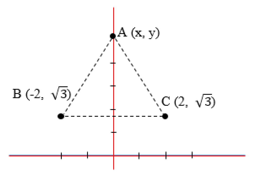
O:= {A, B, C: POINT, ABC: EquilateralTriangle};

$F:= \{\mathrm{B}= (-2, \sqrt{3}),\mathrm{C}= (2, \sqrt{3}\left)\right\}$

G:= {Compute: Distance(A,B)}.

+ Solution for the program:

Set F is split into two sets:

$${\mathrm{F}}_1= \{\mathrm{B}= (-2, \sqrt{3}),\mathrm{C}= (2, \sqrt{3}\left)\right\}$$

F₂ = {Distance(A, B), Distance(B, C), Distance(A, C)}.

By using (O, F₁), the system gets some new facts as follows:

S1: {ABC: EquilateraTtriangle} → {Distance(A,B) = Distance(A,C),

              Distance(A,C) = Distance(B,C),

              Distance(A,B) = Distance(B,C)}

by “Properties of the Equilateral Triangle”.

By using (O, F₂), the system gets some new facts, as follows:

$$\mathrm{S}2:\text{Distance}\left(\mathrm{B},\mathrm{C}\right) = \sqrt{{\left(C.x-\mathrm{B}.\mathrm{x}\right)}^2+{\left(C.y^{°} -\mathrm{B}.y\right)}^2}$$

by “Function of distance”:

$$\mathrm{S}3: \{\mathrm{B}= \left(-2, \sqrt{3}\right),\mathrm{C}= \left(2, \sqrt{3}\right),\text{Distance}\left(\mathrm{B},\mathrm{C}\right) = \sqrt{{\left(C.x-\mathrm{B}.\mathrm{x}\right)}^2+{\left(C.y^{°} -\mathrm{B}.y\right)}^2}\}$$

  → {Distance(B,C) = 4},

by the rule “equation rule for solving an equation”.

Combining those new facts in S1, S2, and S3, the system gets:

S4: {Distance(A,B) = Distance(B,C), Distance(B,C) = 4} → {Distance(A,B) = 4}

Algorithm 4. Prove the equality between two functions.
Given a knowledge domain combining functions K = (C, R, Rules) + Funcs, and a problem P = (O, F) → G on this knowledge domain, with G = {“Prove”: g(x1, x2, …, xn) = h(y1, y2, …, ym)}, where g, h are functions and xi, yj are objects (i = 1…n, j = 1… m).
Input: The problem P = (O, F) → G.
G = {“Prove”: g(x1, x2, …, xn) = h(y1, y2, …, ym)},
with: c ∈ C g: Ic1× Ic2… × Icn→ Ic      xi ∈ Ici, ci ∈ C (1 ≤ i ≤ n)	h: Ib1 × Ib2 …× Ibm → Ic  yk ∈ Ibk, bk ∈ C (1 ≤ k ≤ m)
Output: Solution of the proof: g(x1, x2, …, xn) = h(y1, y2, …, ym).
The idea of the algorithm: It uses Algorithm 3 to compute the values of g(x1, x2, …, xn) and h(y1, y2, …, ym) and compare them. In a case where they cannot be computed, from two sets of objects O1 = {x1, …, xn} and O2 = {y1, …, ym}, the algorithm uses the hypothesis (O1, F) and (O2, F) to determine new facts by applying the algorithm for solving problems on the kernel model, as in Section 3.2.2. Based on those results, it concludes the solution to the current problem.
Step 0: Initialize variables;  flag: = true;  KnownFacts: = F;  O1: = {x1, x2, …, xn};  O2: = {y1, y2, …, ym};  Sol: = [ ]; # solution of the problem. Step 1. Record the elements in the hypothesis and goal. Step 2:  G1: = {“Compute”: g(x1, x2, …, xn)};  G2: = {“Compute”: h(y1, y2, …, ym)};  If problems (O, F) → G1 and (O, F) → G2 are solvable by using Algorithm 4, then:  if the value of g(x1, x2, …, xn) = the value of h(y1, y2, …, ym), then: G   is determined, and go to step 5;  end if; end if; Step 3: Produce new facts based on the hypothesis;  Apply objects and facts in the hypothesis (O, F) to determine new facts by using the algorithm for solving problems on the kernel model, as in Section 3.2;  Update KnownFacts and Sol;	Step 4:  F1: = set of new facts produced from hypothesis (O1, KnownFacts) by using the algorithm for solving problems on the kernel model as Section 3.2  F2: = set of new facts produced from hypothesis (O2, KnownFacts) by using the algorithm for solving problems on the kernel model as Section 3.2  Update Sol;  If (O2 m F1) or (O1 m F2), then:   If statements of g are similar to statements of h, then:    G is determined and update Sol;    Goto step 5;   end if;  end if; Step 5: Conclusion of problem;  If G is determined, then:   Problem (O, F) → G is solvable;  Sol is a solution of the problem;  Reduce the solution found by excluding redundant rules and information in the solution;  Or else: Problem (O, F) → G is unsolvable;  end if;

4.4. Heuristic Rules

For making the inference process faster and more effective, in Algorithms 2–4, some heuristic rules can be used to search the inference rules, as follows:

Hypothesis 1.

Restrict the set of rules that can be applied to the problem.

Based on the facts in the hypothesis of the problem, the reasoning part of the algorithms can reduce the set of rules being searched for the current problem, thus making it faster to search for rules. This heuristic rule is used after the step of recording the hypothesis of the problem in algorithms.

Hypothesis 2.

Arrange the rules in order of priority.

For each kind of practical problem, inference rules are applied in order. Hence, these rules can be arranged according to their priority to speed up the inference process. This heuristic rule is applied when solving sub-problems in algorithms.

5. Application for Intelligent Systems in Education

Intelligent systems in education need useful knowledge bases to organize the complete knowledge in academic courses fully and accurately. The kernel ontology is used to represent the knowledge of matrixes and vectors, such as the structure of matrixes, the relationships between them, and the rules on matrixes. In this section, the method for integrating this knowledge kernel and the knowledge of operators and functions is applied to construct the knowledge bases of linear algebra and graph theory. These knowledge bases are the foundations for designing the intelligent problem solver (IPS) for the corresponding courses, which satisfy the criteria of IPS in mathematics education [23].

5.1. Representation of the Knowledge of Matrixes Using the Kernel Model

The basic knowledge of Matrixes in [13,24] can be represented by the kernel model. It includes the field of real numbers Ñ, the concepts of kinds of matrixes and vectors, and the relationships between these concepts and rules about transforming a matrix:

(C_kernel, R_kernel, Rules_kernel),

C_kernel—set of concepts about matrixes and vectors:

C_kernel = {Matrix, SquareMatrix, DiagnonalMatrix, Vector,}.

The structure of the SquareMatrix concept:

SquareMatrix: Matrix (A square matrix is a matrix);

Attrs: = Matrix.Attrs ∪ {inv, diag, det, sym};

diag: Boolean//the diagonalizable property;

inv: Boolean //the invertible property;

sym: Boolean//the symmetric property;

permutation: Boolean//the property about permutation;

Facts: = {m = n},

RulObj: = Matrix.RulObj ∪ {r1: det # 0 → inv = 1,

r2: ∀ i, j, 1 ≤ i ≤ n, 1 ≤ j ≤ n: a[i][j] = a[j][i] → sym = 1}.

R_kernel—set of relationships between concepts in C_kernel:

R_kernel = {equal (=), similar (~), row equivalence, column equivalence}.

(1)

Relationship “is-a“ between the kinds of matrixes, such as SquareMatrix is-a Matrix.

Rules_kernel—set of inference rules on matrixes.

Example 4.

Rule 1: {A: Matrix, B: Matrix, A.m = B.m, A.n = B.n}:

{∀ i, j, 1 ≤ i ≤ m, 1 ≤ j ≤ n, A.a[i][j] = B.a[i][j]} ↔ {A = B};

Rule 2: {A: SquareMatrix, ∃α ∈ Ñ, ∃m₁, ∃m₂, m₁ ≠ m₂, row_A(m₁) = α * row_A(m₂)}

→ {det(A) = 0};

Rule 3: {A: SquareMatrix, A.permutation = 1}

→ {∃{f₁, …, f_k} is a sequence of row permutation: f₁(f₂(…f_k(this)…)) = I_A.n},

(I_k: the k-order identity matrix, k ∈ ).

5.2. Design Knowledge Base of Linear Algebra Using the Integrating Model (C, R, Rules) + Ops.

5.2.1. Knowledge Base of Linear Algebra

The knowledge about linear algebra was collected from [13,24]. A part of this knowledge domain, about chapters Matrixes–Vectors, Linear Equations System, and Vector Space, can be represented by the model for integrating the kernel and knowledge of operators:

(C, R, Rules) + Ops.

C—set of concepts. Besides concepts in the kernel, C also includes concepts about the Linear Equations System, and Vector Space:

C = C_kernel ∪ {Equation, EquationsSystem, CramerSystem, VectorSpace}.

R—set of relations. Besides the relations in the kernel, R also includes the relationships in the Linear Equations System and Vector Space:

R = R_kernel ∪ {eigenvalue, eigenvector, sub-space, based-set, spanning-set, linearly independent,…}.

Ops is the set of operators between matrixes and vectors, operators in vector space.

Rules is the set of rules on the knowledge domain about linear algebra. It includes rules for generating a new object, equation rules, and equivalent rules in linear algebra.

The knowledge base of this knowledge domain is represented in Appendix A.

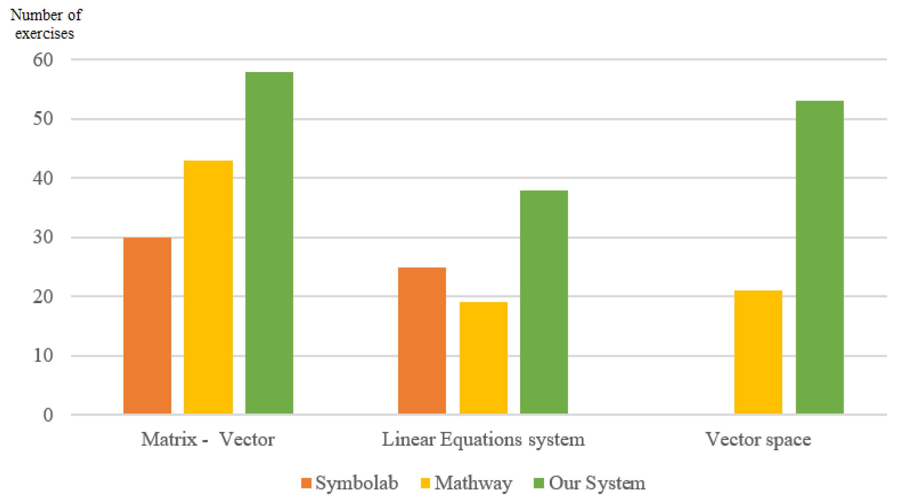
5.2.2. Types of Exercises in Linear Algebra

Based on the knowledge base in Section 5.2.1 and the algorithms in Section 3.2 and Section 4.2.2, an intelligent system for solving problems in linear algebra was designed. Some types of exercises in the curriculum were tested:

• Problems with the Matrix–Vector: Find the rank of a matrix, find the inverse matrix, find the value of an expression between matrixes.
• Problems with the Linear Equations System: Solve a linear equations system by the Gaussian method and Cramer method.
• Problems with the Vector Space: Determine the independence of vectors, determine the basis of a vector space.

Example 5.

Given a set of vectors A = {u = (x₁, x₂, x₃, x₄)∈Ñ⁴|x₁ = 2x₂ = x₃}, and a subspace W = <A>, Determine the based-set of W.

+ The model of this problem:

O: = {W: VectorSpace, x1, x2, x3, x4: Ñ, A: 2Ivector};

F: = {A = {(x1, x2, x3, x4)|x1 = 2x2 , x1 = x3}, A is a spanning-set of W};

G: = {Determine: Based-set of W}.

Step 1: From A = {(x1, x2, x3, x4)|x1 = 2x2, x1 = x3},  let u: Vector:   u = (x1, x2, x3, x4), u ∈ A. Step 2: From u = (x1, x2, x3, x4), u ∈ A,    A = {(x1, x2, x3, x4)|x1 = 2x2, x1 = x3},  then u = (x1, ½.x1, x1, x4). Step 3: From u = (x1, ½.x1, x1, x4),  then u = (x1, ½.x1, x1, 0) + (0, 0, 0, x4),    u = (1, ½, 1, 0) *x1 + (0, 0, 0, 1) *x4. Step 4: From u = (1, ½, 1, 0) *x1 + (0, 0, 0, 1) *x4,   let a1: Vector, a2: Vector,    a1 = (1, ½, 1, 0) a2 = (0, 0, 0, 1).

Step 5: Let B = {a1 = (1, ½, 1, 0), a2 = (0, 0, 0, 1)},  then B is linearly independent. Step 6: From u = (1, ½, 1, 0) *x1 + (0, 0, 0, 1) *x4,   u ∈ A, x1 ∈ Ñ, x4 ∈ Ñ,   a1 = (1, ½, 1, 0), a2 = (0, 0, 0, 1),   B = {a1, a2},   A is a spanning-set of W, then B is a spanning-set of W. Step 7: From B is a spanning-set of W,    B is linearly independent.  Then, B is a based-set of W

5.3. Design Knowledge Base of Graph Theory Using the Integrating Model (C, R, Rules) + Funcs

5.3.1. Knowledge Base of Graph Theory

The knowledge about graph theory was collected from [25,26,27]. In this section, we only cover the knowledge about undirected graphs. The knowledge base of this knowledge domain can be represented by the method for integrating the kernel and knowledge of functions:

(C, R, Rules) + Funcs.

C—set of concepts. It includes concepts in the kernel and concepts about the knowledge of the graph:

C = C_kernel ∪ {Graph, Connected Graph, Simple Graph, …}.

R—set of relationships. Besides relationships in the kernel, R also includes relationships between graphs:

R = R_kernel ∪ {sub-graph, isomorphism,…}.

Funcs—set of functions of the knowledge domain about graph theory:

Funcs = {Degree, Path, Girth, EulerPath, HamiltonCycle …}.

Rules—set of rules on the knowledge domain about graph theory. It includes deductive rules and equivalent rules.

The knowledge base of this knowledge domain is represented in Appendix B.

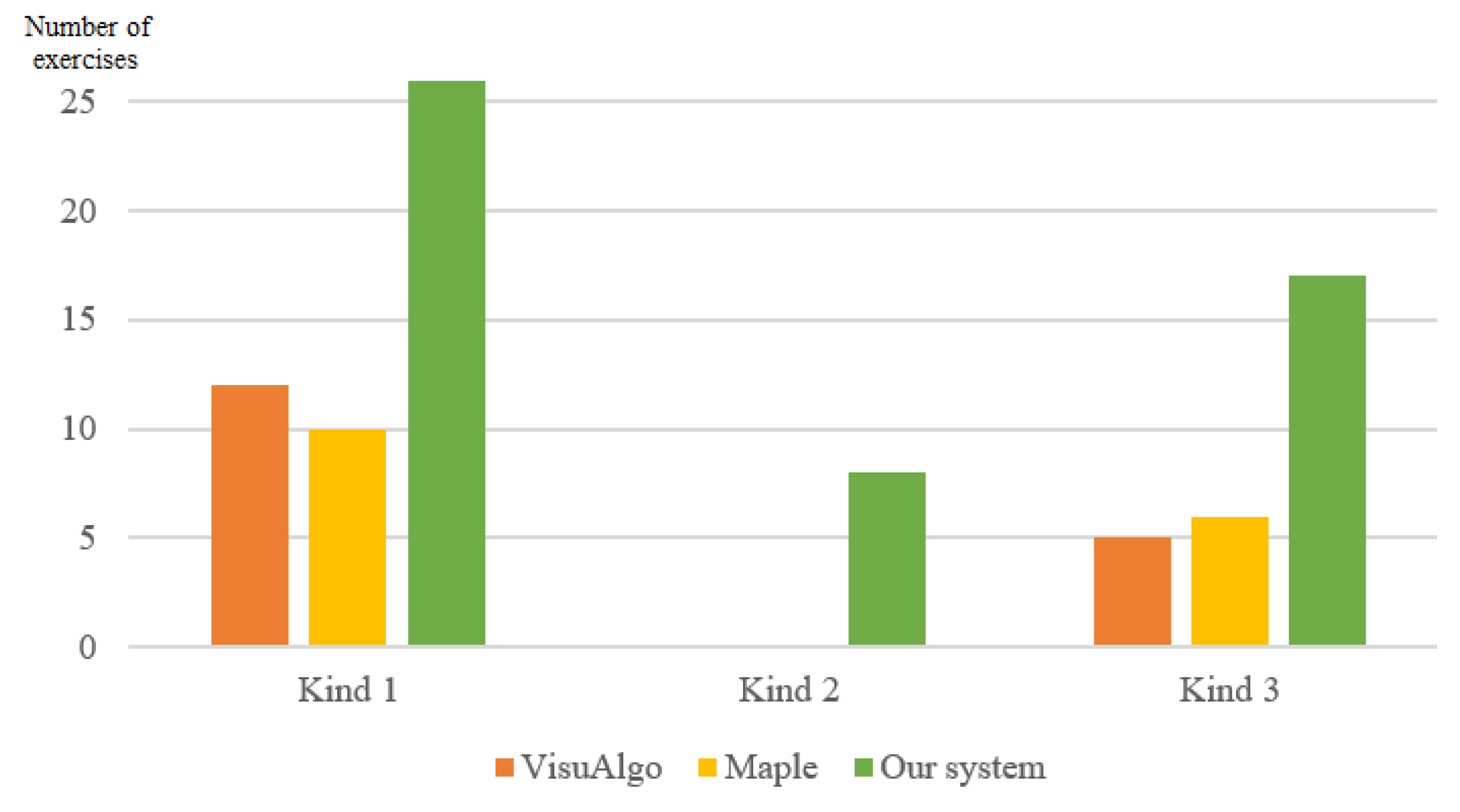
5.3.2. Kinds of Exercises in Graph Theory

Based on the knowledge base and the inference engine in the above section, an intelligent system for solving problems in graph theory was designed. This system can solve many types of problems that are in the curriculum of this course. They are classified in the three following types [18]:

• Type 1: find the shortest paths between nodes in a graph, find a minimum spanning tree for a weighted undirected graph. These problems also have additional conditions;
• Type 2: Determine a graph from an expression of graphs;
• Type 3: Prove a property of a graph or a relationship between two graphs.

Example 6.

Given two simple graphs G₁, G₂, as in Figure 5, prove G₁ and G₂ are isomorphic.

+ The model of this problem:

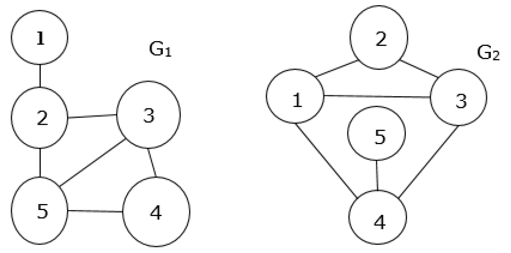
O: = {G1, G2: Graph},

F: = {G1.Adj = {(0, 1, 0, 0, 0), (1, 0, 1, 0, 1), (0, 1, 0, 1, 1), (0, 0, 1, 0, 1), (0, 1, 1, 1, 0)},

G2.Adj = {(0, 1, 1, 1, 0), (1, 0, 1, 0, 0), (1, 1, 0, 1, 0), (1, 0, 1, 0, 1), (0, 0, 0, 1, 0)},

G: = {“Prove”: G1 and G2 are isomorphic}

+ The solution of this system:

Step 1: From G₁: Graph, G₁. Adj = $\left(\begin{array}{ccccc}0& 1& 1& 1& 0\\ 1& 0& 1& 0& 0\\ 1& 1& 0& 1& 0\\ 1& 0& 1& 0& 1\\ 0& 0& 0& 1& 0\end{array}\right)$,

Select P₅: SquareMatrix,

 P₅ = $\left(\begin{array}{ccccc}0& 0& 0& 0& 1\\ 0& 0& 0& 1& 0\\ 1& 0& 0& 0& 0\\ 0& 1& 0& 0& 0\\ 0& 0& 1& 0& 0\end{array}\right)$, P₅.n = G₁.n, P₅.permutation = 1.

Step 2:

From P₅ = $\left(\begin{array}{ccccc}0& 0& 0& 0& 1\\ 0& 0& 0& 1& 0\\ 1& 0& 0& 0& 0\\ 0& 1& 0& 0& 0\\ 0& 0& 1& 0& 0\end{array}\right)$,

Then T: SquareMatrix, T = Transpose(P₅), T = $\left(\begin{array}{ccccc}0& 0& 1& 0& 0\\ 0& 0& 0& 1& 0\\ 0& 0& 0& 0& 1\\ 0& 1& 0& 0& 0\\ 1& 0& 0& 0& 0\end{array}\right)$.

Step 3:

From P₅ = $\left(\begin{array}{ccccc}0& 0& 0& 0& 1\\ 0& 0& 0& 1& 0\\ 1& 0& 0& 0& 0\\ 0& 1& 0& 0& 0\\ 0& 0& 1& 0& 0\end{array}\right)$, T = $\left(\begin{array}{ccccc}0& 0& 1& 0& 0\\ 0& 0& 0& 1& 0\\ 0& 0& 0& 0& 1\\ 0& 1& 0& 0& 0\\ 1& 0& 0& 0& 0\end{array}\right)$,

G₁.Adj = $\left(\begin{array}{ccccc}0& 1& 0& 0& 0\\ 1& 0& 1& 0& 1\\ 0& 1& 0& 1& 1\\ 0& 0& 1& 0& 1\\ 0& 1& 1& 1& 0\end{array}\right)$, G₂.Adj = $\left(\begin{array}{ccccc}0& 1& 1& 1& 0\\ 1& 0& 1& 0& 0\\ 1& 1& 0& 1& 0\\ 1& 0& 1& 0& 1\\ 0& 0& 0& 1& 0\end{array}\right)$,

Then G₁. Adj = P₅ * G₂. Adj * T

Step 4: From G₁: Graph, G₂: Graph, P₅: SquareMatrix, T: SquareMartrix,

G₁.n = G₁.n, P5.n = G₁.n, T = Transpose(P₅),

G₁. Adj = P₅ * G₂. Adj * T

Then, G₁ and G₂ are isomorphic.

6. Experimental Results

6.1. Intelligent Problem Solver in Linear Algebra

The integrating model between the kernel ontology and the knowledge of operators was used to design the knowledge base of IPS in linear algebra, as in Section 5.2. The knowledge base of this system satisfied the criteria of the knowledge representation for an IPS in education [27]. It can be used to support the study of Linear Algebra at university.

Symbolab is a website which can automatically solve mathematical problems [28]. It can solve several problems about matrixes and equation systems, and produce step-by-step solutions. Mathway is another website to solve linear algebra problems automatically [29]. It plays as a chatbot to interact with the user. The test results of Symbolab, Mathway, and our system are shown in

Table 4. The results of testing of exercises in [13].

Chapter	Number of Testing Problems	Number of Problems that Can Be Solved
		Symbolab	Mathway	Our System
Matrix–Vector	65	30	43	58
Linear Equations system	39	25	19	38
Vector space	67	0	21	53
Total	171	55	83	149

and Figure 6.

The knowledge bases of Symbolab and Mathway are organized as frames. They only can solve some types of exercises, which have already been set up. The interface of Mathway is a chatbot for showing the step-by-step solutions. Besides this, the user can input some simple problems by images to that program. In contrast, the knowledge base of our program was organized as a complete system, representing the knowledge similarly to the knowledge acquisition of human. Its solutions were clear, step-by-step, and similar to those of students.

The IPS in linear algebra was also examined by the students in two universities. In the curriculum for information technology from these two universities, linear algebra takes place in the second semester of the first academic year. This survey focused on four requirements of an IPS in education [27,30]: sufficient knowledge base, the ability to solve common exercises, pedagogy, usefulness. Each criterion can be evaluated from 1–5, from very bad to very good. The meaning of each level was described in [30].

There were 87 students in this survey, who were either:

• First-year students (63 students ~72%): students who took this course the first time;
• The other students (24 students ~28%): students who took this course again because they had failed before.

Each student was prompted to choose three problems from a list of 149 exercises that could be solved by the program. After seeing the program-generated solutions for those problems, they were requested to input three more problems using specification language and then check the solutions produced by the program. Based on these results, the students evaluated this program by four criteria, on a scale of 1 to 5.

The results of this survey are shown in

Table 5. Results of the survey.

Criterion	Level
	1	2	3	4	5
Sufficient knowledge	25%			75%
Ability to solve common exercises	24%			76%
Pedagogy	32%			68%
Usefulness	31%			69%

.

6.2. Intelligent Problem Solver in Graph Theory

The integrating model between kernel ontology and the knowledge of functions was used to design the knowledge base of IPS in graph theory, as in Section 5.3. The knowledge base of this system meets requirements of an IPS in education [23]. The students used this system to support their learning of graph theory at university.

VisuAlgo is a learning website [31] that can visualize algorithms in graph theory, such as graph traversal, finding the minimum spanning tree, shortest paths, graph matching, traveling salesman. Maple software is an essential mathematical tool for education [32]. It includes many packages for studying mathematics. Maple has a network package to represent the knowledge of graph theory. Although it can solve some problems about graphs, Maple only shows their results, and not step-by-step solutions.

Table 6. The ability for solving exercises in graph theory [27].

Kind of Exercises	Number of Testing Exercises	Number of Problems that Can Be Solved
		VisuAlgo	Maple	Our System
Type 1	28	12	10	26
Type 2	11	0	0	8
Type 3	25	5	6	17
Total	64	17	16	51

and Figure 7 compare the ability for solving exercises in graph theory [27] between VisuAlgo, Maple, and our system.

With exercises of type 1, our system can solve problems with additional conditions, while VisuAlgo and Maple can only solve algorithms which do not contain conditions. Exercises of type 2 and type 3 are difficult for students. VisuAlgo only solves some exercises in type 3 about determining the ismorphism between two graphs, but our system could solve exercises of all types. Maple only shows the results of exercises and not the detailed solutions. It is a useful tool to support learning, but it does not meet the requirements of an IPS in graph theory.

Similar to the IPS in linear algebra, the IPS in graph theory was also examined by the students in two universities, based on four criteria: sufficient knowledge base, the ability to solve common exercises, pedagogy, and usefulness. In the curriculum for information technology from these two universities, graph theory took place in the first semester of the first academic year.

A total of 95 students joined this survey, and were again classified into two types: students who were studying this course for the first time (73 students ~77%), and students who were studying the course for the second time (22 students ~23%).

Each student was again prompted to pick three exercises in the list of 51 exercises that could be solved by the program. After seeing the program-generated solutions for those problems, they were asked to input three more problems using the specification language and then check the solutions produced by the program. Based on these results, the students evaluated this program by four criteria on a scale of 1 to 5. Results of this survey are shown in

Table 7. Results of the survey.

Criterion	Level
	1	2	3	4	5
Sufficient Knowledge	25%			75%
Ability to solve common exercises	24%			76%
Pedagogy	15%			85%
Usefulness	26%			74%

:

7. Conclusions and Future Works

Knowledge integration is an important method for developing intelligent software. It makes the system more intelligent than conventional systems. Systems with knowledge integration can simulate the knowledge organization and solve problems on the knowledge domains in a similar way to the human method. In this paper, a method for knowledge integration based on ontology was presented. This method is effective at representing the real knowledge domain. It meets the requirements of knowledge integration. The integrating models have a kernel consisting of concepts, relationships, and inference rules, which can be extended with other knowledge by integrating more components, kinds of facts, and kinds of rules into the kernel. Hence, a method for integration between the knowledge kernel and the knowledge of operators and functions was proposed. These models can represent real knowledge domains more clearly, naturally, and accurately, and therefore are applicable in practice.

These integrating models were applied to build IPSs in mathematical courses at universities, such as linear algebra and graph theory. The kernel of these models represented the concepts of matrixes and vectors, relationships, and inference rules on them. Based on this kernel, the integrating model with knowledge of operators was used to represent the knowledge base of linear algebra, consisting of additional knowledge about matrix operators, linear equations systems, and vector spaces. Besides this, this kernel was also integrated with the knowledge of functions and operators to represent and organize the knowledge base of graph theory. These knowledge bases were applied to build the IPSs for these courses. These systems supported students well in their study of these courses. They could solve common exercises in each course, and their reasoning and solutions were readable, step-by-step, and similar to human methods.

Our method for integrating the knowledge based on ontology can be applied to other knowledge domains, especially knowledge in natural sciences, such as mathematics, physics, and chemistry. Depending on the knowledge domains, knowledge bases may vary in their structure, as long as the structure is bounded to these following five elements: concepts, relationships, inference rules, operators, and functions. This setup makes the integration of multiple knowledge bases seamless and consistent.

In the future, we will research and develop more methods and techniques of knowledge integration that are applicable in more complex real-world knowledge domains. Problems using heuristics and sample problems [21] for reasoning on the integrated structure will also be studied. Additionally, with the IPS in education, after finding the solution of a problem, the system will omit the redundant steps, which are unnatural for humans, and wrap the solution steps into tutoring steps. This stage of the system uses the meta-knowledge of humans, especially the knowledge of the learner. In the next study, some meta-knowledge will be researched to process the final solutions of the system. This will make the solutions more natural and tend to the instructions for solving a problem.

Nowadays, there are many knowledge domains collected from many sources. Hence, a model to represent the combination of multiple knowledge domains is very necessary for knowledge integration, and a method to combine multiple knowledge models will have many applications in practice.

References

1. Noy, N.; McGuinness, D. Final Report on the 2013 NSF Workshop on Research Challenges and Opportunities in Knowledge Representation; National Science Foundation Workshop Report: Alexandria, VA, USA, 2013. [Google Scholar]
2. Mehta, N.; Bharadwaj, A. Knowledge Integration in Outsourced Software Development. J. Manag. Inf. Syst. 2015, 32, 82–115. [Google Scholar] [CrossRef]
3. Wolfram|Alpha. Available online: https://www.wolframalpha.com/ (accessed on 7 September 2019).
4. IMS Learning Information Services Tools. Available online: https://www.k-int.com/products/ims-learning-information-services-tools/ (accessed on 7 September 2019).
5. Bassetta, M.; Fatta, F.; Manti, A. San Pietro di Deca in Torrenova: Integrated Survey Techniques for the Morphological Transformation Analysis. In Handbook of Research on Emerging Technologies for Architectural and Archaeological Heritage; IGI Global: Hershey, PA, USA, 2017. [Google Scholar]
6. Sowa, J.F. Knowledge Representation: Logical, Philosophical, and Computational Foundations; Brooks Cole: Pacific Grove, CA, USA, 2000. [Google Scholar]
7. Gayathri, R.; Uma, V. Ontology based knowledge representation technique, domain modeling languages and planners for robotic path planning: A survey. ICT Express 2018, 4, 69–74. [Google Scholar]
8. Truong, H.B.; Duong, T.H.; Thanh, N.N. A hybrid method for fuzzy ontology integration. Cyber. Syst. Int. J. 2013, 44, 133–154. [Google Scholar] [CrossRef]
9. Provine, R.; Schlenoff, C.; Balakirsky, S.; Smith, S.; Uschold, M. Ontology-based methods for enhancing autonomous vehicle path planning. Robot Auton. Syst. 2004, 49, 123–133. [Google Scholar] [CrossRef]
10. Fratini, S.; Nogueira, T.; Policella, N. Integrating modeling and knowledge representation for combined task, resource and path planning in robotics. In Proceedings of the Workshop on Knowledge Engineering for Planning and Scheduling—27th International Conference on Automated Planning and Scheduling (ICAPS 2017), Pittsburgh, PA, USA, 18–23 June 2017. [Google Scholar]
11. Ong, J.; Remolina, E.; Prompt, A.; Robinson, P.; Sweet, A.; Nishikawa, D. Software testbed for developing and evaluating integrated autonomous systems. In Proceedings of the 2015 IEEE Aerospace Conference, Big Sky, MT, USA, 7–14 March 2015; pp. 1–12. [Google Scholar]
12. Do, N.V. Ontology COKB for Knowledge Representation and Reasoning in Designing Knowledge-Based Systems. In Communications in Computer and Information Science (CCIS); Springer: Berlin/Heidelberg, Germany, 2015; Volume 513, pp. 101–118. [Google Scholar]
13. Anton, H.; Rorres, C. Elementary Linear Algebra, 10th ed.; John Wiley & Sons: Hoboken, NJ, USA, 2010. [Google Scholar]
14. Dumontier, M.; Baker, C.J.; Baran, J.; Callahan, A.; Chepelev, L.; Cruz-Toledo, J.; Del Rio, N.R.; Duck, G.; Furlong, L.I.; Keath, N.; et al. The Semanticscience Integrated Ontology (SIO) for biomedical research and knowledge discovery. J. Biomed. Semant. 2014, 5, 14. [Google Scholar] [CrossRef] [PubMed]
15. Chabeb, Y.; Tata, S.; Belaïd, D. Toward an integrated ontology for Web services. In Proceedings of the 2009 Fourth International Conference on Internet and Web Applications and Services, Venice/Mestre, Italy, 24–28 May 2009; pp. 463–467. [Google Scholar]
16. Bobillo, F.; Straccia, U. fuzzyDL—An Expressive Fuzzy Description Logic Reasoner. In Proceedings of the 2008 IEEE International Conference on Fuzzy Systems, Hong Kong, China, 1–6 June 2008; pp. 923–930. [Google Scholar]
17. Bang, T.H.; Quach, X.H. An Overview of Fuzzy Ontology Integration Methods Based on Consensus Theory. In Advanced Computational Methods for Knowledge Engineering; Van Do, T., Le Thi, H.A., Nguyen, N.T., Eds.; Springer: Berlin/Heidelberg, Germany, 2014; Volume 282, pp. 217–227. [Google Scholar]
18. Do, N.V.; Nguyen, H.D.; Mai, T.T. Intelligent Educational Software in Discrete Mathematics and Graph Theory. In Proceedings of the 17th International Conference on Intelligent Software Methodologies, Tools, and Techniques (SOMET 2018), Granada, Spain, 26–28 September 2018; Volume 303, pp. 925–938. [Google Scholar]
19. Munir, K.; Anjum, M.S. The use of ontologies for effective knowledge modelling and information retrieval. Appl. Comput. Inform. 2018, 14, 116–126. [Google Scholar] [CrossRef]
20. Do, N.V.; Nguyen, H.D.; Selamat, A. Knowledge-Based model of Expert Systems using Rela-model. Int. J. Softw. Eng. Knowl. Eng. (IJSEKE) 2018, 28, 1047–1090. [Google Scholar] [CrossRef]
21. Do, N.V.; Nguyen, H.D.; Mai, T.T. Designing an Intelligent Problems Solving System based on Knowledge about Sample Problems. In Proceedings of the 5th Asian conference on Intelligent Information and Database Systems (ACIIDS 2013), Kuala Lumpur, Malaysia, 18–20 March 2013; Volume 7802, pp. 465–475. [Google Scholar]
22. Nguyen, H.D.; Do, V.; Pham, V.T.; Inoue, K. Solving problems on a knowledge model of operators and application. Int. J. Digit. Enterp. Technol. (IJDET) 2018, 1, 37–59. [Google Scholar] [CrossRef]
23. Nguyen, H.D.; Do, N.V.; Tran, N.P.; Pham, X.H. Criteria of a Knowledge model for an Intelligent Problems Solver in Education. In Proceedings of the 10th IEEE International Conference on Knowledge and Systems Engineering (KSE 2018), Ho Chi Minh City, Vietnam, 1–3 November 2018; pp. 288–293. [Google Scholar]
24. Lang, S. Linear Algebra, 3rd ed.; Undergraduate Texts in Mathematics; Springer: Berlin/Heidelberg, Germany, 2004. [Google Scholar]
25. Fournier, J. Graph Theory and Applications—With Exercises and Problems; Wiley Online Library: Hoboken, NJ, USA, 2010. [Google Scholar]
26. Chartrand, G.; Zhang, P. A first Course in Graph Theory; Dover Pub.: Mineola, New York, NY, USA, 2006. [Google Scholar]
27. Mier, A.; Maureso, M. Graph Theory: Exercises and Problems; Barcelona School of Informatics: Barcelona, Spain, 2015. [Google Scholar]
28. Symbolab. Available online: www.symbolab.com (accessed on 7 September 2019).
29. Mathway. Available online: https://www.mathway.com/LinearAlgebra (accessed on 7 September 2019).
30. Nguyen, H.D.; Do, N.V. Intelligent Problems Solver in Education for Discrete Mathematics. In Proceedings of the 16th International Conference on Intelligent Software Methodologies, Tools, and Techniques (SOMET_17), Kitakyushu, Japan, 26–28 September 2017; Volume 297, pp. 21–34. [Google Scholar]
31. VisuAlgo. Available online: https://visualgo.net/en (accessed on 7 September 2019).
32. Maple Software. Available online: https://www.maplesoft.com/ (accessed on 7 September 2019).
Figure 1. Structure of the knowledge kernel.
Applsci 09 03793 g001
Figure 2. Integrating the kernel and the knowledge of operators and functions.
Applsci 09 03793 g002
Figure 3. Problem P1.
Applsci 09 03793 g003
Figure 4. Problem P2.
Applsci 09 03793 g004
Figure 5. Graphs in example 6.
Applsci 09 03793 g005
Figure 6. Results of testing of Symbolab, Mathway, and our system.
Applsci 09 03793 g006
Figure 7. Results of testing of VisuAlgo, Maple, and our system.
Applsci 09 03793 g007