Abstract
To provide theoretical basis for cavitation noise control, the cavitation evolution around a hydrofoil and its induced noise were numerically investigated. A modified turbulence model and Zwart cavitation model were employed to calculate the flow field and predict the cavitation phenomenon accurately. Then, the acoustic analogy method based on the Ffowcs Williams-Hawking (FW-H) equation was applied to analyze the cavitation-induced noise. Seven cavitation numbers were selected for analysis. Acoustic power spectral density (PSD) and acoustic pressure were investigated to establish the relationship between cavitation number and their acoustic characteristics. It was indicated that as cavitation number decreases, cavitation cycle length gets shorter and the magnitude of acoustic power spectral density increases dramatically. One peak value of acoustic power spectral density induced by the extending and retracting of leading-edge cavitation can be obtained under sheet cavitation conditions, while under cloud cavitation, two peak values of acoustic power spectral density can be obtained and are induced by superposition from leading-edge cavitation and trailing vortex.
1. Introduction
Cavitation mainly occurs in the location where the local pressure of the liquid drops below the threshold value at a specified temperature. As the phenomenon occurs in a wide range of hydraulic engineering situations where liquid flowing systems are involved, cavitation sways numerous industries, such as petroleum transportation and the water pump industry. What is more, cavitation can generate destructive behavior. From previous experience, the effects of cavitation are various, such as causing pitting of the boundary surface and leading to vibration and noise problems. Therefore, fully investigating and understanding the mechanism of cavitation is essential for its widespread and undesirable features.
In the last several decades, different experimental and numerical methods have been applied to the research of cavitation. Cavitation in various structures and characteristics has been studied by many investigators.
Experimental studies generally observe the occurrence of a cavitation phenomenon and its hydrodynamic characteristics using a high-speed video camera. Guo [1] observed the process of bubble occurrence, development, and collapse. This research elucidated the mechanism of bubble evolution of the high-speed centrifugal pump. There have also been some experimental observations around hydrofoils carried out by Peng [2] in the cavitation tunnel to explain the spatial–temporal evolution of cloud cavitation. They found that U-type flow structures are common in cloud cavities, and sheet cavities always have a convex–concave profile. The shedding is generally caused by the converging re-entrant flows, which occur in the convex part, and the re-entrant flows are normal to the contour edge. Liang [3] experimentally investigated the particle motions induced by bubble cavitation. They clearly recorded and analyzed the cavitation bubble dynamics and its induced particle moving dynamics. The results revealed that the distance between the particle and the cavitation bubble is an important influence factor in this phenomenon. Zhang [4] focused on the collapsing mechanism of a laser-induced cavitation bubble between a spherical particle and a solid wall. The influences of several paramount parameters were discussed in this paper. Hao [5] used a high-speed camera to capture and observe the cavitation flow patterns in different stage. The study revealed the significant effect of different material on the cavitation flow. Gao [6] experimentally analyzed the characteristics of the cavitation pattern and the vibration response around an NACA66 hydrofoil.
Numerical approaches have also been presented and applied to efficiently investigate the cavitation phenomena. Among the most notable studies, Ji [7] focused on the mechanism of the interaction between the fluid vortex production and cavitation. The analysis of the flow field showed that cavitation promotes vortex formation and increases the boundary layer thickness with the flow unsteadiness. Huang [8] studied the turbulent vortex–cavitation interactions in transient sheet and cloud cavitation phenomena. Their analysis of the vorticity transport equation revealed a strong correlation between the cavity and vorticity structure. The interaction between the leading edge and trailing edge vortices was significantly changed by the transient development of sheet and cloud cavitation. Yu [9] compared three widespread cavitation models in the evolution around an NACA0015 hydrofoil based on the level set method. The results offer the optimal selection of cavitation models at different conditions. Liu [10] investigated the cavitation phenomenon around the asymmetric leading edge (ALE) 15 hydrofoil through large eddy simulation, and the modified Schnerr–Sauer cavitation model was employed, which considers the influence of incompressible gas. Peng [11] numerically analyzed the strong and weak interactions between neighboring cavitation bubbles with a revised single-component multiphase Lattice Boltzmann method. The mutual interaction among a cluster of cavitation bubbles was also investigated. Guo [12] analyzed the inner flow field of the axial pump to reveal the cavitation mechanism. The results showed that cavitation performance is enhanced by positive inlet guide vane angles but hampered by negative ones.
So many works have focused on cavitation evolution in recent years, but little attention has been paid to cavitation noise. Cavitation-induced noise is an essential issue to be solved. Some research about different hydraulic machinery has been proposed. Lee and Seung-jae [13] experimentally measured the noise for a three-dimensional hydrofoil at different attack angles. Seol [14] investigated the relationship between the cavitation patterns and flow-induced noise for a model propeller through experiments. Li [15] conducted an experiment in a contraction–divergence channel to investigate the bubble pattern and cavitation noise under different liquid speeds. Numerical approaches have also been applied to investigate cavitation noise. Jung [16] focused on an acoustic analogy based on a classical theory of Fitzpatrik a Strasberg to verify the direct simulation and analyze the source of noise. Sanghyeon Kim [17] investigated the effects of cavitation-flow patterns of hydrofoils, with an emphasis on turbulence models, and corresponding radiated noise was analyzed. Zhang [18] transformed bubble volume pulse to propeller cavitation noise using the Lighthill equation.
Previous investigations on cavitation focused mainly on engineering applications, such as cavitation noise in hydro turbine and pump, but the mechanism has not been reflected and its control measures are mainly based on engineering experiences. Also, cavitation is an intricate phenomenon. With changes in boundary conditions, the morphology and patterns of cavitating vary a lot. Thus, the characteristics of noise radiated by cavitating flow are complex. Previous studies on cavitation noise are limited, and the mechanism and acoustic characteristics of different cavitation numbers have not been fully investigated. What is more, the cavitation number in different hydraulic engineering situations changes a lot. To be specific, the characteristics of noise induced by a quadrupole acoustic source, dipole acoustic source, and monopole acoustic source vary greatly with changes in cavitation numbers. To identify the source of noise and restrict the complex noise from different acoustic sources in various hydraulic engineering situations, a deeper understanding of the fundamental mechanism of cavitation-induced noise is essential.
Thus, the present research focuses on this problem and figures out the mechanism and characteristics of cavitation-induced noise. The present study analyzes different acoustic characteristics of noise induced by the cavitation flow around an NACA0015 hydrofoil through numerical methods. Specifically, the numerical simulations are performed by the commercial software FLUENT. The filter-based turbulence model (FBM) and Zwart cavitation model were employed to calculate the flow field and accurately predict the cavitation phenomenon, while the acoustic analogy method based on the FW-H equation was applied to analyze the flow-induced noise with different cavitation numbers. Based on this research, the control measures can be improved to be more specific and effective.
2. Mathematical Model
2.1. Basic Equations
The continuity equation and momentum equation of water vapor and liquid water under a humongous assumption are as follows:
where ρm is the density of the mixture, u is time-averaged velocity, and p is relative pressure. μm is the mixture molecular viscosity and μt is turbulent viscosity, based on the Boussinesq hypothesis.
2.2. FBM Model
Cavitating flow is a fully developed turbulent phenomenon which has a mass transfer between two phases. The standard k-ε model is favored because of its low requirements for computing resources and stable calculating result. However, the widely used k-ε turbulence model is mainly based on a steady average flow, where the viscosity coefficient is calculated by turbulent kinetic energy and turbulent dissipation rate. This indicates that the turbulence scale calculated by the k-ε model is very large and the excessive forecast of viscous coefficient affects the accuracy. So, this article adopted the filter-based model (FBM) to optimize the k-ε model. The viscosity coefficient of FBM is defined as:
where FFBM represents the filter function and λ represents the filter scale. This article takes Cμ to be 0.09 and C3 to be 1.0.
2.3. Zwart Cavitation Model
The mass transport equation for vapor can be written as follows:
where the ρv represent the vapor density and αv is the vapor volume fraction.
The Zwart Model is derived from the simplified Rayleigh–Plesset Equation, which describes the bubble dynamics. This model’s evaporation source terms and condensation source terms are as follows:
where R represents bubble diameter, rnuc represents nucleation site volume fraction, Fe represents evaporation coefficient, Fc represents condensation coefficient, and Pv represents vaporization pressure. This article set these coefficients as follows: R = 1.0 × 10⁻⁶ m, rnuc = 5.0 × 10⁻⁴ m, Fe = 50, Fc = 0.01.
2.4. FW-H Equation
The acoustic analogy method is the key to solve flow-induced noise. This method is based on the FW-H Equation, which is widely accepted in engineering. The FW-H Equation is derived from the continuity equation and the N-S equation:
where p’ represents sound pressure, δ(f) represents the Dirac-δ function, and Tij represents the Lighthill stress tensor.
The three terms on the right side of the FW-H equation represent the quadrupole acoustic source, dipole acoustic source, and monopole acoustic source, respectively. The quadrupole acoustic source expresses high-frequency noise radiated by the hydrofoil boundary layer and vortex shedding. The dipole acoustic source expresses low-frequency noise radiated by the unsteady pulsating force, which is induced by an inhomogeneous flow field and the turbulent flow field around the hydrofoil surface. The monopole acoustic source expresses noise induced by bubble development and collapse. To hydrofoil cavitation, the quadrupole acoustic source is far less than the other two acoustic source. Thus, this article ignored the quadrupole acoustic source.
3. Computational Domain and Boundary Conditions
The NACA0015 hydrofoil, with chord length C = 0.07 m, was selected and its angle of attack was α = . Figure 1 shows the shape of the computational domain and the boundary conditions. The inlet boundary was 3 C ahead of the hydrofoil, where the inflow velocity was fixed, Vx = 7.2 m/s (Re = 5.62 × 10⁵). The outlet boundary was 5.5 C behind the hydrofoil, and a pressure outlet was set to control the cavitation number by setting different pressures. The span wise was 0.1 C. The water-tunnel wall and the hydrofoil surface were set as the no-slip wall boundary condition. Twenty-one monitor points were set around the hydrofoil to monitor pressure pulsation. Their locations are shown in Figure 2. Monitor points were arranged at intervals of 0.1 C along the upper surface of the hydrofoil. Their names were U0, U1, U2, U3, U4, U5, U6, U7, U8, U9, U10, B1, B2, B3, B4, B5, B6, B7, B8, B9, and B10, in order.
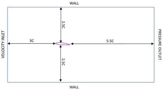
Figure 1.
Computational domain and boundary conditions.
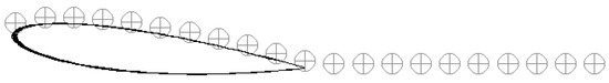
Figure 2.
Monitor points.
Structural mesh was adopted in the simulation. The mesh near the leading-edge and the tail was refined deliberately to precisely capture the complex characteristics of the fierce flow change. To control the overall nodes of the mesh, the mesh density of the other parts of the flow field was reduced appropriately. After the grid independence validation, the total mesh nodes were set as 946,082. The mesh distribution of the computational domain is shown in Figure 3.
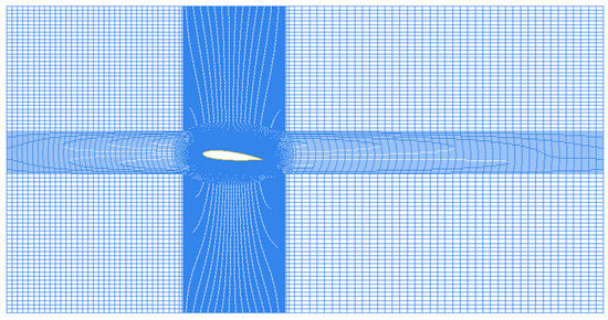
Figure 3.
Mesh distribution of the computational domain.
In the present study, seven different cavitation numbers with different cavitation types were selected, and are summarized in Table 1.

Table 1.
Computational conditions.
4. Results and Discussion
In the present study, seven different cavitation numbers with different cavitation types (i.e., no cavitation, sheet cavitation, and cloud cavitation) were selected and used to investigate the characteristics of cavitation induce noise.
4.1. Sheet Cavitation
4.1.1. Verification Test
Simulations in this article were conducted by ANSYS FLUENT to solve the flow field numerically. The time step in the calculation was set as 1.0 × 10⁻⁴ s and the maximum calculated frequency of the corresponding acoustic response was 5 kHZ. Before the characteristic of sheet cavitation was investigated, a case with σ = 1.075 was first simulated and compared with experimental data to verify the accuracy of the simulation. The contours of the vapor volume fraction around the hydrofoil from the simulation are shown in Figure 4, along with the corresponding experimental data. As shown in Figure 4, sheet cavitation clung to the leading edge steadily. The cavitation developed and extended from the leading edge towards the flow direction, and the change was not obvious. The simulated frequency of morphology evolution was about 11 HZ, which is in accordance with the experimental result. It can be seen in Figure 4 that the cavitation phenomenon in photos from a high-speed video camera was highly similar to the simulation result, and the exactness of the simulation is therefore proven.
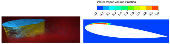
Figure 4.
Numerical results and experimental data for σ = 1.075.
4.1.2. Sheet Cavitation Flow-Induced Noise
Figure 5 shows the acoustic pressure level in the flow field at two different times, and 21 different locations separated on and behind the hydrofoil were selected. Since the cavity was relatively steady, the acoustic pressure changed little at different times. Thus, the magnitude of acoustic pressure was identical at different times. The results show that the peak values of acoustic pressure at different times shared the same characteristic, that the distance between peak values of acoustic pressure and cavitation was 0.2–0.4 C. Besides this, it is shown in the figure that acoustic pressure dropped abruptly in the point behind the tail. This change was largely due to the rapid dissipation of pressure fluctuation behind the hydrofoil tail.
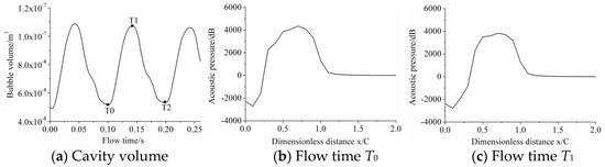
Figure 5.
Acoustic pressure at different flow times for σ = 1.075.
The frequency spectrogram of leading noise in point U7 is shown in Figure 6. Only one peak value, at 10.68 HZ, can be observed, which was due to the extending and retracting of leading-edge cavitation. It is worth mention that the cycle length was 93.60 ms, which corresponded with the peak value of the frequency spectrogram.
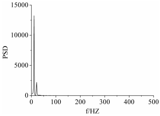
Figure 6.
Acoustic power spectral density at U7 for σ = 1.075.
The advent time of the peak value at different points of the hydrofoil was also investigated, and is shown in Figure 7. The peak values of different points occurred sequentially in time from point U5 to U8, which was the result of cavitation growth in the leading-edge. Besides this, the result verifies the rule that the distance from locations of peak value of acoustic pressure in a specific time is 0.2–0.4 C away from cavitation growth points.
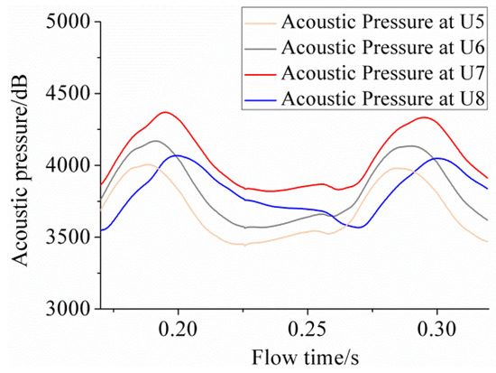
Figure 7.
Acoustic pressure pulsation at different locations for σ = 1.075.
4.1.3. Influences of Different Sheet Cavitation Number
In the comparably steady flow condition of sheet cavitation, three different cavitation numbers, σ = 0.975, σ = 1.075, and σ = 1.175, were investigated and their similarities and disparities are discussed in this part.
Cavitation morphology for σ = 0.975 shared several features with cloud cavitation because of its relatively lower outlet pressure. It can be seen from Figure 8, Figure 9, Figure 10 and Figure 11 that cavitation clung to the leading-edge, instead of shedding from the leading edge periodically, but cavitation developed and extended from the leading edge towards the flow direction dramatically. Thereafter, cavitation retreated and collapsed. As a contrast, cavitation for σ = 1.075 and σ = 1.175 stayed constant and cavity stretched from the leading-edge to approximately 1/3 C. Additionally, the rule that the distance from locations of peak value in specific times is 0.2–0.4 C away from cavitation growth and the collapsing point was again verified.
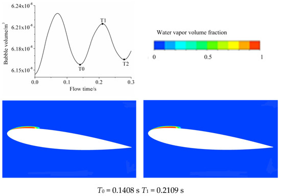
Figure 8.
Bubble volume pulsation and numerical results for σ = 1.175.
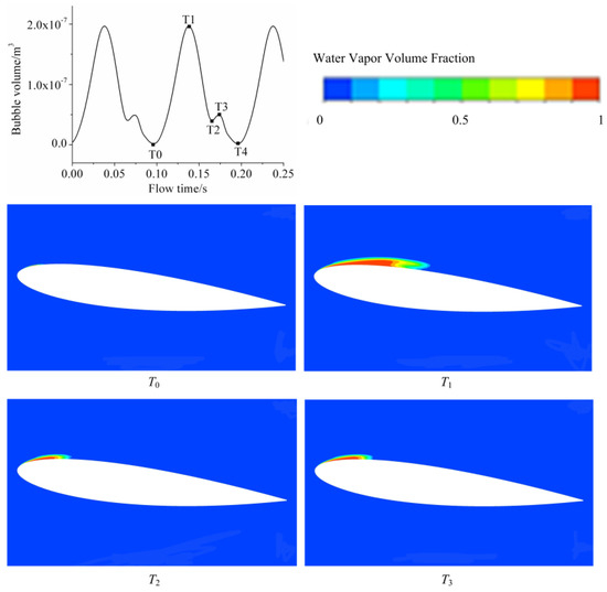
Figure 9.
Bubble volume pulsation and numerical results for σ = 0.975.
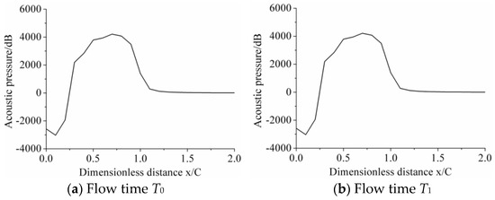
Figure 10.
Acoustic pressure at different flow times for σ = 1.175.
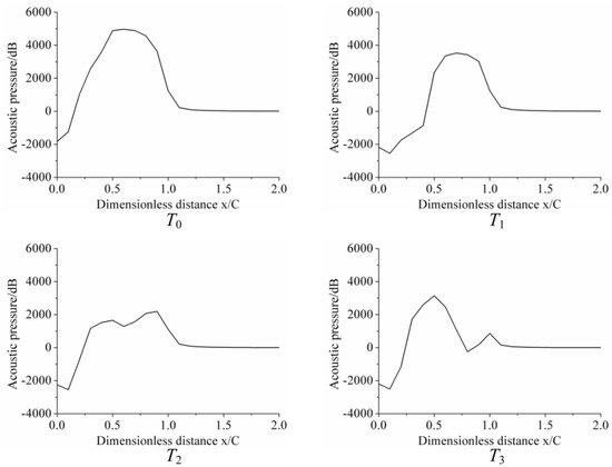
Figure 11.
Acoustic pressure at different flow times for σ = 0.975.
Frequency spectrograms of leading noise for three different cavitation numbers are shown in Figure 12, and the same point was selected for analysis.
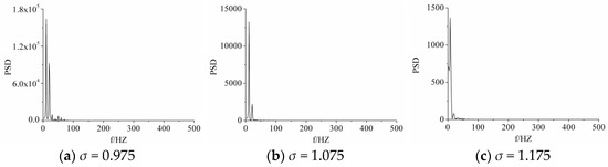
Figure 12.
Acoustic power spectral density at U7 for σ = 0.975, 1.075, and 1.175.
The frequency of the first peak value for σ = 1.175 was 7.28 HZ, and the frequency of the first peak value for σ = 1.075 and σ = 0.975 was 10.49 HZ. Therefore, the cycle lengths for σ = 0.975, σ = 1.075, and σ = 1.175 were 95.33 ms, 95.22 ms, and 137.36 ms, respectively. In addition to the period length, there was also a difference in the magnitude of acoustic power spectral density. The magnitude of acoustic power spectral density for σ = 1.075 and σ = 1.175 were the same, whereas that for σ = 0.975 was significantly higher. The results of PSD had good agreement with the experimental research from Harish Ganesh [19], that the magnitude of multimodal behavior increases with decreasing cavitation number. The difference was largely due to its drastic pressure fluctuation caused by extending and retreating of cavitation on the leading edge.
4.2. Cloud Cavitation
4.2.1. Verification Test
Eight specific moments in a whole cycle are shown in Figure 13, with corresponding experimental data. The period of the cavitation evolution cycle was approximately 57.7 ms, which corresponds to the evolution cycle in the experiment results. Compared with numerical results, the experimental data show the numerical results are in good agreement.
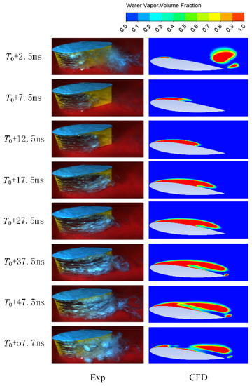
Figure 13.
Numerical results and experimental data.
4.2.2. Cloud Cavitation Flow-Induced Noise
The acoustic pressure level of 21 different locations in the flow field at different times is shown in Figure 14. They shared the same characteristic that the distance from the locations of peak value in the designated time is about 0.2–0.4 C away from cavitation growth and collapsing points. Besides this, the characteristic of cloud cavitation was identical to that of sheet cavitation.
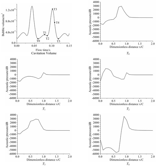
Figure 14.
Acoustic pressure at different flow times for σ = 0.65.
Frequency spectrograms of leading noise are shown in Figure 15. For point U5, two peak values at 17.09 Hz and 34.19 Hz are the results of superposition from leading edge cavitation and trailing vortex. For point B6, only one peak value at 17.09 Hz can be observed. The reason for this is that the impact of leading-edge cavitation dissipated over such a long distance from collapsing point to point B6. The peak value at 17.09 Hz was the impact of shedding cavitation, which can be verified by the simulation results in Figure 13, that shedding cavitation occurred once a cycle.
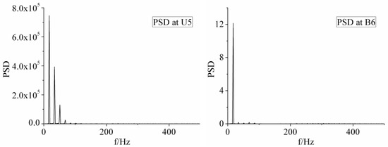
Figure 15.
Acoustic power spectral density at U5 and U6 for σ = 0.65.
The evident disparity of peak acoustic pressure value from point U2–U5 is shown in Figure 16. The results indicate that the distance from locations of peak value in specific times were 0.2–0.4 C away from cavitation growth and collapsing points, which corresponds with the analysis above. Additionally, the peak value of different points occurred successively in time from point U2 to U5, the result of cavitation growth in the leading-edge.
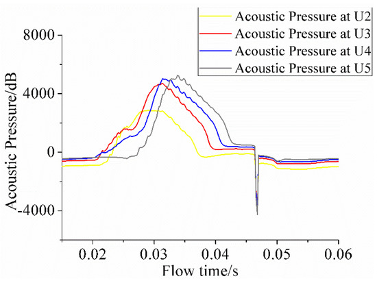
Figure 16.
Acoustic pressure pulsation at different locations for σ = 0.65.
4.2.3. Influences of Different Cloud Cavitation Number
In the complex flow condition of cloud cavitation, three different cavitation numbers were investigated and their similarities and disparities are discussed in this part.
Figure 17 and Figure 18 show the acoustic pressure level at different locations at different times, and three different cavitation numbers are considered. It is noteworthy that point U10, located in the tail of the hydrofoil, presented a relatively higher acoustic pressure during the collapse of either the front bubbles or trailing vortex. Besides this, Figure 19 indicates that the pressure fluctuation at point U10 was significantly higher than other points nearby, for instance, T2. Therefore, higher pressure fluctuation was presumably the cause for the peak acoustic pressure value at U10.
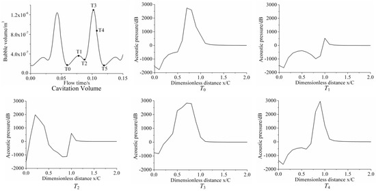
Figure 17.
Acoustic pressure at different flow times for σ = 0.55.
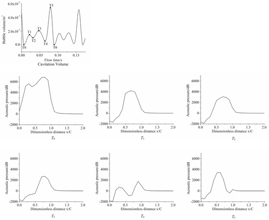
Figure 18.
Acoustic pressure at different flow times for σ = 0.75.
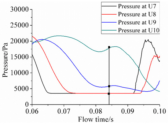
Figure 19.
Pressure pulsation at U7, U8, U9, and U10 for σ = 0.65.
Figures of acoustic power spectral density (PSD) of three different cavitation numbers are presented. Note that the same position was selected in different conditions. When σ = 0.55, the frequency of the second peak, which represents the growth and collapsing of front bubbles, was about twice as much as that of the first peak, which represents the growth and collapse of the trailing vortex. To be specific, the growth and collapsing of the trailing vortex occurred once a cycle, but that of the front bubbles happened twice in one cycle.
When σ = 0.65, the frequency and magnitude of the first and second peak were almost the same as that of σ = 0.55.
When σ = 0.75, a difference can be observed that the frequency of the second peak was three times higher than that of the first peak, and that means the growth and collapsing of leading-edge cavitation occurred three times a cycle. Additionally, the first peak was relatively higher than that of σ = 0.55 and σ = 0.65, which are in good correlation with the phenomenon that the collapsing of trailing vortex and front bubbles occurs at the same time, as shown in Figure 20.
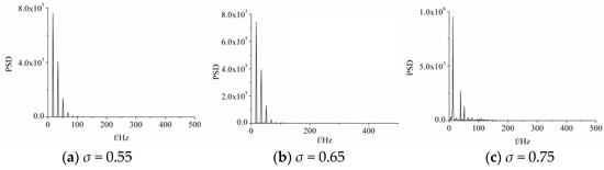
Figure 20.
Acoustic power spectral density for σ = 0.55, 0.65, and 0.75.
4.3. Comparison of Non-Cavitation, Sheet Cavitation, and Cloud Cavitation
In this part, σ = 3.3, σ = 1.075, and σ = 0.65, which are typical examples of non-cavitation, sheet cavitation, and cloud cavitation, respectively, were investigated and are discussed.
Figure 21 shows the leading noise frequency spectrograms of three kinds of cavitation phenomenon. It can be observed in the figure that as cavitation number decreased, cavitation cycle length became shorter and the magnitude of acoustic power spectral density increased dramatically. The cause can be attributed to their difference in cavitation morphology. For σ = 3.3, no water vapor was detected, which means there was no periodic change, such as growth and collapsing in cavitation morphology. Thus, the magnitude of acoustic power spectral density was extremely small. Nonetheless, high-frequency acoustic power spectral density still existed. For sheet cavitation and cloud cavitation, as cavitation number decreased, unsteady characteristic became more evident, and the vortex shedding and collapse were more violent. Therefore, the magnitude of acoustic power spectral density increased.
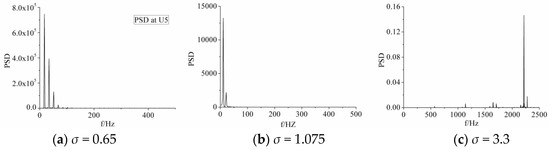
Figure 21.
Acoustic power spectral density at U7 for σ = 0.65, 1.075, and 3.3.
For σ = 3.3, higher acoustic pressure can be observed in Figure 22. Figure 23 shows the pressure fluctuation for three different cavitation numbers. As we can see in the figure, the magnitude of pressure for σ = 3.3 was clearly larger compared with that of other cavitation numbers. Pressure fluctuation was possibly the cause of acoustic pressure. Note that point U5 reached the peak value of acoustic pressure. Combined with what is elucidated above that acoustic pressure drop abruptly in the point behind the tail, the reason may be that the peak value at U5 was the result of superposition from the upper surface of the hydrofoil.
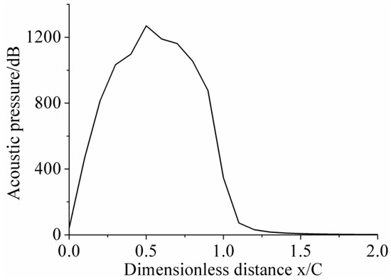
Figure 22.
The variation in acoustic pressure along the hydrofoil surface for σ = 3.3.
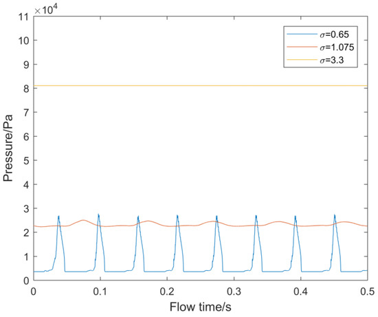
Figure 23.
Pressure pulsation at U5 for σ = 0.65, 1.075, and 3.3.
5. Conclusions
In this study, the cavitation evolution around a hydrofoil and its acoustic characteristic of flow induced noise were numerically investigated. The filter-based turbulence model and Zwart cavitation model were employed to accurately calculate the flow field and predict the cavitation phenomenon. Besides this, an acoustic analogy method based on the FW-H equation was applied to analyze the flow-induced noise. To research the regularities and features of hydrofoil in different cavitation conditions, seven cavitation numbers were selected and investigated.
- (1)
- In the comparison of non-cavitation, sheet cavitation, and cloud cavitation, it can be observed that as cavitation number decreases, cavitation cycle length gets shorter and the magnitude of acoustic power spectral density increases dramatically. The cause can be contributed to their difference in cavitation morphology. For σ = 3.3, higher acoustic pressure can be observed, meanwhile, the magnitude of pressure for σ = 3.3 is clearly larger compared with that of other cavitation numbers. Thus, it is speculated that pressure fluctuation is possibly the cause of high acoustic pressure for the condition of non-cavitation;
- (2)
- For the condition of sheet cavitation, the distance from the location of peak value in the designated time is 0.2–0.4 C away from the cavitation growth and collapsing point. Only one peak value of acoustic power spectral density, which was due to the extending and retracting of the leading-edge cavitation, could be observed;
- (3)
- For the condition of cloud cavitation, the results show that the distance between peak values of acoustic pressure and cavitation is 0.2–0.4 C. Besides this, acoustic pressure drops abruptly in the point behind the tail. For point upper surface of the hydrofoil, two peak values of acoustic power spectral density are the result of superposition from the leading-edge cavitation and trailing vortex. As a comparison, for points behind the hydrofoil, only one peak value can be observed, for the reason that the impact of leading-edge cavitation has dissipated over such a long distance from the collapsing point. Differences in PSD for different cavitation numbers were also observed. When σ = 0.55 or σ = 0.65, the peak value of acoustic power spectral density reveals that the growth and collapsing of trailing vortex occurs once a cycle, but that of front bubbles happen twice in one cycle. When σ = 0.75, the growth and shedding of leading-edge cavitation occur three times a cycle. Additionally, the first acoustic power spectral density peak is relatively higher, which is caused by the phenomenon that the collapsing of the trailing vortex and front bubbles occurs at the same time.
Author Contributions
Conceptualization, A.Y. and D.Z.; Methodology, Q.T. and H.C.; Validation, A.Y., and D.Z.; Formal analysis, A.Y.; Investigation, X.W. and Z.Z.; Writing-original draft preparation, X.W. and Z.Z; Writing-review and editing, A.Y.; Supervision, A.Y.; Funding acquisition, A.Y.
Funding
This research was funded by the National Natural Science Foundation of China (Project No. 51806058) and the Fundamental Research Funds for the Central Universities (Project No. 2019B15014).
Conflicts of Interest
The authors declare no conflict of interest.
References
- Guo, X.M.; Zhu, L.H.; Zhu, Z.C.; Cui, B.L.; Li, Y. Numerical and experimental investigations on the cavitation characteristics of a high-speed centrifugal pump with a splitter-blade inducer. J. Mech. Sci. Technol. 2015, 29, 259–267. [Google Scholar] [CrossRef]
- Peng, X.X.; Ji, B.; Cao, Y.T.; Xu, L.H.; Zhang, G.P.; Luo, W.; Long, X.P. Combined experimental observation and numerical simulation of the cloud cavitation with U-type flow structures on hydrofoils. Int. J. Multiph. Flow 2016, 79, 10–22. [Google Scholar] [CrossRef]
- Lv, L.; Zhang, Y.X.; Zhang, Y.N. Experimental investigations of the particle motions induced by a laser-generated cavitation bubble. Ultrason. Sonochem. 2019, 56, 63–76. [Google Scholar] [CrossRef] [PubMed]
- Zhang, Y.N.; Xie, X.Y.; Zhang, Y.N.; Zhang, Y.X.; Du, X.Z. Experimental study of influences of a particle on the collapsing dynamics of a laser-induced cavitation bubble near a solid wall. Exp. Therm. Fluid Sci. 2019, 105, 289–306. [Google Scholar] [CrossRef]
- Hao, J.F.; Zhang, M.D.; Huang, X. Experimental Study on Influences of Surface Materials on Cavitation Flow Around Hydrofoils. Chin. J. Mech. Eng. 2019, 32, 45. [Google Scholar] [CrossRef]
- Gao, Y.; Huang, B.; Wu, Q.; Wang, G.Y. Experimental investigation of the vibration characteristics of hydrofoil in cavitating flow. Chin. J. Theor. Appl. Mech. 2015, 47, 1009–1016. [Google Scholar]
- Ji, B.; Luo, X.W.; Arndt, R.E.A.; Wu, Y.L. Numerical simulation of three dimensional cavitation shedding dynamics with special emphasis on cavitation-vortex interaction. Ocean Eng. 2014, 87, 64–77. [Google Scholar] [CrossRef]
- Huang, B.; Zhao, Y.; Wang, G.Y. Large Eddy Simulation of turbulent vortex-cavitation interactions in transient sheet/cloud cavitating flows. Comput. Fluids 2014, 92, 113–124. [Google Scholar] [CrossRef]
- Yu, A.; Tang, Q.H.; Zhou, D.Q. Cavitation Evolution around a NACA0015 Hydrofoil with Different Cavitation Models Based on Level Set Method. Appl. Sci. 2019, 9, 758. [Google Scholar] [CrossRef]
- Liu, M.; Tan, L.; Cao, S.L. Cavitation-Vortex-Turbulence Interaction and One-Dimensional Model. Renew. Energy 2019, 139, 1159–1175. [Google Scholar] [CrossRef]
- Peng, C.; Tian, S.C.; Li, G.S.; Michael, C.S. Simulation of multiple cavitation bubbles interaction with single-component multiphase Lattice Boltzmann method. Int. J. Heat Mass Trans. 2019, 137, 301–317. [Google Scholar] [CrossRef]
- Guo, Z.W.; Pan, J.Y.; Qian, Z.D.; Ji, B. Experimental and numerical analysis of the unsteady influence of the inlet guide vanes on cavitation performance of an axial pump. Proc. Inst. Mech. Eng. Part C-J. Mech. 2019, 233, 3816–3826. [Google Scholar] [CrossRef]
- Lee, S.J. Experimental Study on the Cavitation Noise of a Hydrofoil. J. Soc. Nav. Archit. Korea 2007, 44, 111–118. [Google Scholar] [CrossRef]
- Seol, H. Experimental Study on the Cavitation Noise Characteristics of Model Propeller in Uniform Inflow. Trans. Korean Soc. Noise Vib. Eng. 2018, 28, 728–734. [Google Scholar] [CrossRef]
- Li, C.; Ying, C.F.; Bai, L.X. The characteristic of cavitation noise and the intensity measurement of hydrodynamic cavitation. Sci. Sin. Phys. Mech. Astron. 2012, 42, 987–995. [Google Scholar] [CrossRef]
- Seo, J.H.; Moon, Y.J.; Shin, B.R. Prediction of cavitating flow noise by direct numerical simulation. J. Comput. Phys. 2008, 227, 6511–6531. [Google Scholar] [CrossRef]
- Kim, S.; Cheong, C.; Park, W.G. Numerical investigation on cavitation flow of hydrofoil and its flow noise with emphasis on turbulence models. AIP Adv. 2017, 7, 065114. [Google Scholar] [CrossRef]
- Zhang, Y.K.; Xiong, Y. Numerical Method for Predicting Ship Propeller Cavitation Noise. In Proceedings of the 30th Chinese Control Conference, Yantai, China, 22–24 July 2011. [Google Scholar]
- Ganesh, H.; Wu, J.; Ceccio, S. Flow-Induced Noise of Shedding Partial Cavitation on a Hydrofoil. In Proceedings of the FLINOVIA 2017: Flinovia—Flow Induced Noise and Vibration Issues and Aspects-II, State College, PA, USA, 27–28 April 2017; pp. 61–69. [Google Scholar]
© 2019 by the authors. Licensee MDPI, Basel, Switzerland. This article is an open access article distributed under the terms and conditions of the Creative Commons Attribution (CC BY) license (http://creativecommons.org/licenses/by/4.0/).