Article

Computer Vision Measurement of Pointer Meter Readings Based on Inverse Perspective Mapping

School of Mechanical and Aerospace Engineering, Jilin University, Changchun 130000, China
*
Author to whom correspondence should be addressed.
Appl. Sci. 2019, 9(18), 3729; https://doi.org/10.3390/app9183729
Submission received: 22 July 2019 / Revised: 2 September 2019 / Accepted: 3 September 2019 / Published: 6 September 2019
(This article belongs to the Section Computing and Artificial Intelligence)

Abstract

:
A computer vision method for measuring multiple pointer meters is proposed based on the inverse perspective mapping. First, the measured meter scales are used as the calibration objects to obtain the extrinsic parameters of the meter plane. Second, normal vector of the meter plane can be acquired by the extrinsic parameters, obtaining the rotation transformation matrix of the meter image. Then, the acquired meter image is transformed to a position both parallel to the meter plane and near the main point by the rotation transformation matrix and the extrinsic parameters, eliminating the perspective effect of the acquired image. Finally, the transformed image is tested by the visual detection method to obtain the readings of the pointer meter, improving measurement precision. The results of the measurement verify the effectiveness and accuracy of the method.

1. Introduction

Pointer meters are used to measure temperature, pressure, flow, level and digital display. Compared with digital instruments, the pointer meters have the advantages of reliable structure, low cost and intuitive readability. Especially in industrial measurement such as substation automation or petrochemical industry, the pointer meters are more likely to observe rapid changes in measured values. Therefore, operators often use the pointer meters to observe measurement process. In general, the readings of the pointer meters are obtained by person judging. With the development of automation and intelligent technology, industry pays attention to that the computer vision methods measure the pointer meter readings. Although modern imaging techniques [1,2,3,4] have increased image resolution, the measuring accuracy is still affected by several factors, such as angle or distance of the camera observing the meters. Therefore, it is essential to utilize the computer vision techniques to measure the pointer meter in order to improve the accuracy and convenience of measurement.
Generally, present methods of the pointer meter measurement can be divided into two kinds of models. One is extracting the critical points of measured meters display to calibrate the reading. In 1994, Robert et al. [5] detected image of the circular arc scales to obtain values of a meter using Hough transform. And the values on the rectangle frame were obtained visually by detecting the two lines. In 2000, F. Corrêa Alegria [6] proposed combining image processing with computer vision techniques to automatically measure the readings of analog instruments, improving measurement stability compared to human eye discrimination reading. Using edge extraction and pattern recognition technology, Shutao Zhao et al. [7] dealt with images of the meters to achieve automatically reading of the power meter data in 2005. An automatic verification system [8] of dial indicators was investigated by the image subtraction and dynamic threshold segmentation of features of the dashboard image in 2008. Using the edge detection and mathematical morphology, Zhijia Zhang [9] screened out image region in the pointers, and then pointer positions were located by the structure and position characteristics in 2009. A modified active shape models scheme [10] for automatic measuring of multiple analog meters had been proposed in 2014. The analog meter reading scheme utilized different feature points, and appropriately modeled of its displacement according to analog meter scales. In 2018, Yifan Ma [11] proposed to use the analysis based on the binarization threshold to segment the pointer region, solving the problem of the pointer shadow. And a random sample consensus method put forward to overcome background image interference.
The other model uses a parametric perspective imaging model to convert the pixel coordinates to object space locations. At the Centre for Metrology and Accreditation in Finland, Hemming et al. [12] came up with computer vision based device for calibrating meter readings in 2002, and calculated the measurement uncertainty. In 2007, they also updated the equipment developed to a micrometer calibration device [13]. By the Canny edge detection, Danilo Alves de Lima [14] investigated a vision system for both calibrating the instruments and obtaining the readings in 2008. Using the computer vision, Fernandez et al. [15] presented a model for calibrating portable measurement devices in 2009. In order to automatically calibrate analog meter measurement process, two segmentation-free methods were presented by P. A. Belan [16] in 2013. Bresenham algorithm and Radial projection were applied to identify the location of the pointer of the analog meter so that the readings of the analog meter can be automatically obtained. In 2014, an automatic identification model for pointer meters based on binocular vision was developed by Yang. Use two cameras located on the left and right side of the pointer meter in the model. The two pointer lines obtained from the left and right images were then rebuild in three dimensions to determine the value of the point instrument [17]. In 2018, real-time measurement of multi-pointer instrument was realized by using ARM (Advanced RISC Machine) Hisilicon mobile processing platform and skeleton extraction technology based on distance transform algorithm [18].
In summary, there are advantages and disadvantages in the measurement methods of the above two models. The first model has the advantage of being easier to measure the reading of the pointer meter, however, the measurement accuracy is lower. If the meter surface is not parallel to the image plane, the changes of the image locations are critical points shown by Figure 1. The measurement accuracy of the second model is greatly improved, but the redundancy parameters also greatly increase the computational complexity and limit its application and promotion.
The present method calibrates the extrinsic parameters by the pixel coordinates and world coordinates of the mid-points of the measured meter scales firstly, and then the meter image is made parallel to the surface of the meter by the inverse perspective mapping. The mapping is finished by rotation transformation of the meter image, and the rotation transformation matrix obtained by the Rodrigues formula. The rest of the paper is arranged as follows: the approach of measurement the reading of the pointer meter is presented in Section 2. Section 3 provides experiments and results, and analyzes the effects of certain factors through experiments. Conclusions are given in Section 4.

2. Measurement Principle

2.1. Reverse Projection of the Meter Image

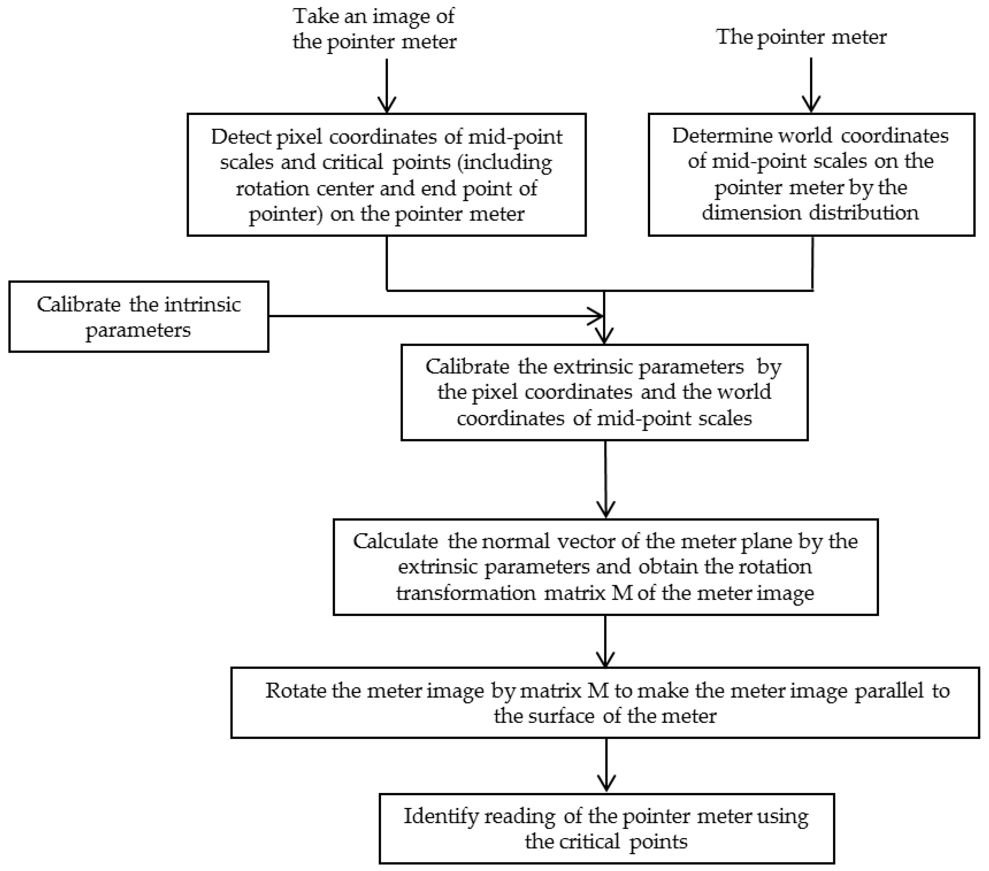
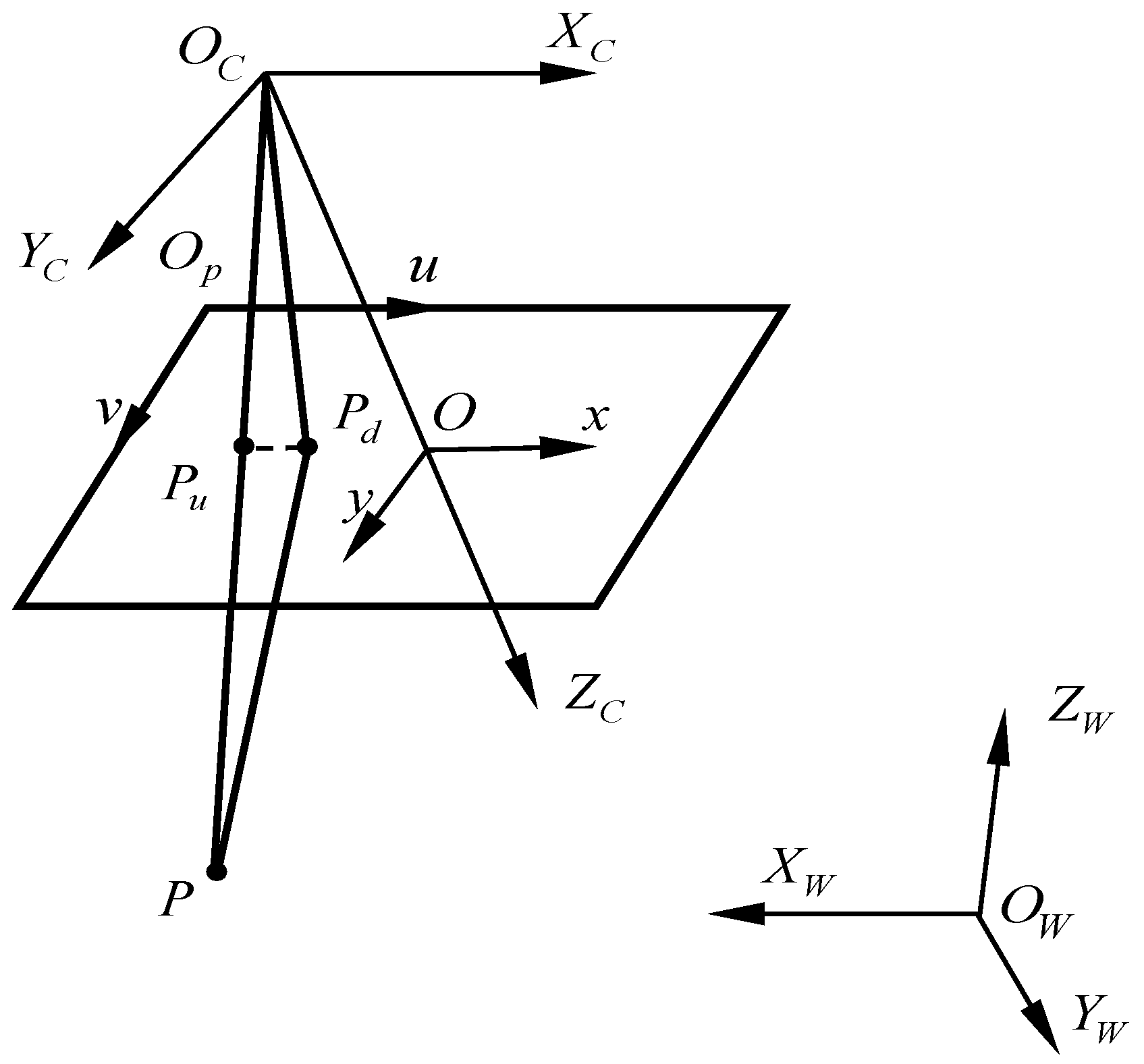
The present method for measuring readings of the pointer meter is shown in Figure 2. The camera intrinsic parameters A are calibrated by the Zhang [19] in the Appendix for the detail. For obtaining the extrinsic parameters, XwYw coordinate plane of a World Coordinate System (WCS) is established on the meter surface, direction of the Xw-axis is parallel to connection line from center of the pointer rotation to the starting scale, the Zw axis perpendicular to the meter surface, and origin of the World Coordinate System is at center of the pointer rotation. Radii of circular arc of the scale distribution and center angles corresponding to the distribution can be determined by manually measuring the dimension distribution of the meter scales. So, world coordinates of midpoint on every short scale can be calculated by the radius r s and angles as:
X W i = r S × cos ( γ × i ) Y W i = r S × sin ( γ × i ) Z W i = 0
Here γ is center angle between neighbors two scales, i is the scale.
Then, the sub-pixel coordinates ( u , v ) T of midpoint of each short scale on the meter image can be detected by sub-pixel detection algorithm [20]. The camera extrinsic parameters [ R , T ] are determined by the world and pixel coordinates of the midpoints. And the world coordinates of midpoints on the short scales are transformed into the camera coordinates ( X C i , Y C i , Z C i ) T by the extrinsic parameters.
For transforming the meter image parallel to the meter surface by the inverse perspective mapping, normal vector k = [ k x , k y , k z ] of the meter surface is calculated by the camera coordinates of three midpoints to obtain angle θ between k and normal vector of the meter’s theoretical image plane. So, the inverse perspective mapping is finished by rotating the meter’s theoretical image plane to the angle θ relative to k . From the Rodrigues formula, the rotation transformation matrix M for the image plane is obtained by k :
M = [ k x 2 k y k x k z k x k x k y k y 2 k z k y k x k z k y k z k z 2 ]
The meter image is rotated by the matrix M to make the meter image parallel to the surface of the meter. The coordinate of the point ( X i , Y i , Z i ) T in the meter image is transformed by M to the coordinates of the points ( x i , y i , z i ) T in the transformed meter image, as shown in Equation (3).
[ x i y i z i ] = M [ X i Y i Z i ]
Here, the z i of all the points in the transformed image are the same. Therefore, the coordinates of the critical point (including the rotation center and the endpoint of the pointer) in the transformed meter image can be corrected in this way, identifying the reading of the pointer meter.

2.2. Measuring Readings of Pointer Meters

The reading of the pointer meter can be obtained by locating the position of the pointer relative to the scale lines after the inverse perspective mapping. The algorithm for measuring the pointer meter reading is divided into two main steps. In the first step, all the midpoints of scales on the pointer meter are detected in order from zero scale line to the maximum scale line. In the next step, the critical points on the pointer meter are collected separately. Then, the reading of the pointer meter is identified.
First of all, the obtained pointer meter image is converted into the binary image by the method [21] to obtain automatically the meter dial. It uses the adaptive threshold to segment the image and use the connected domain labeling to locate the dial and the scale lines from the background pixels. Due to uneven illumination of the pointer meter dial or digital printing on the pointer meter, it is possible to be a few defective scale lines in the detected area. So, morphological opening and closing can reduce image noise by eliminating the bright or dark components [
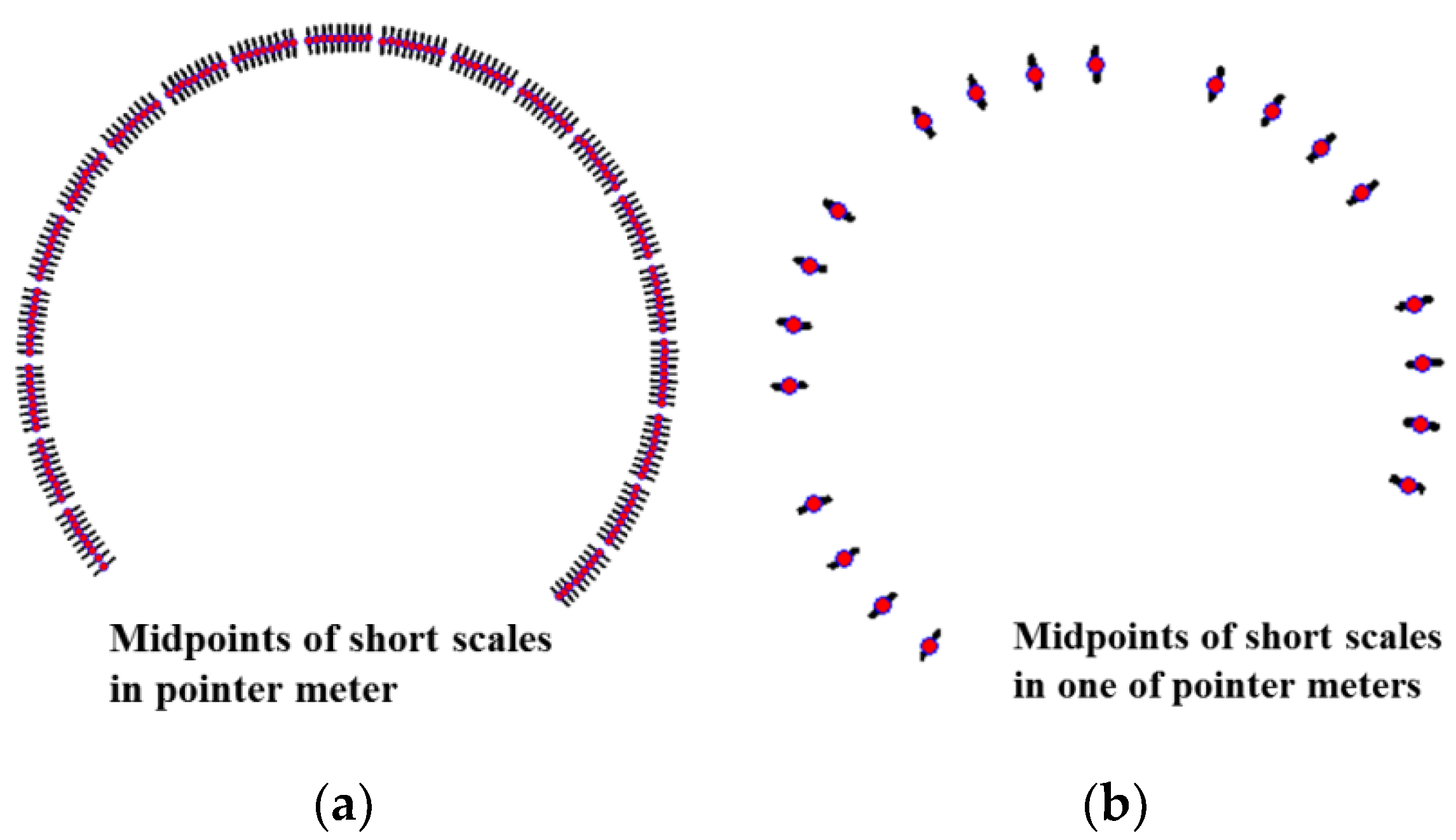
22]. And then, all the mid-points of the scales lines are detected from zero-scale line p 1 ( x 1 , y 1 ) to maximum-scale line p M ( x M , y M ) .
After detecting all the midpoints of the short scales, one circle is fitted to these points, and the coordinate of the rotation center c ( x c , y c ) can be obtained by circle fitting algorithm [23]. Then, the Hough transformation method [24] is adopted to detect the straight lines in the image, the longest straight line that intersects the coordinates of the rotation center can be determined as the position of the pointer. Therefore, the coordinate of the endpoint of the pointer e ( x e , y e ) 
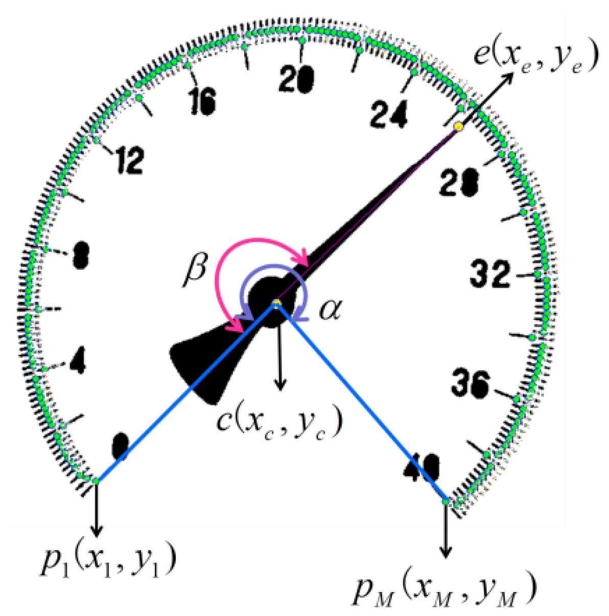
on the pointer meter can be acquired. Finally, the reading of the pointer meter can be calculated by the Angle method, which calculates the angle between the zero scale line and the detected pointer according to Equation (4):
a n g l e ( α ) = arctan y 1 y c x 1 x c arctan y c y M x c x M a n g l e ( β ) = arctan y e y c x e x c arctan y c y 1 x c x 1 v a l u e = a n g e l ( β ) × s c a l e v a l u e ( N ) a n g e l ( α )
Here, α was the premeasured angle between zero scale line and the maximum scale line. In order to calibrate the extrinsic parameter of the meter plane, the angle α is manually premeasured by the dimension distribution of the pointer meter scales. When the measurement is carried out by the present method, the meter image is firstly made parallel to the meter surface by the inverse mapping, then angle α on the image is obtained by the pixel coordinates of the midpoints of the scale line and the rotation center, and the pixel coordinates are determined by the sub-pixel detection of the transformed image. β was the angle between the detected pointer and zero scale line. N is the scale value which is measured between zero scale line p 1 ( x 1 , y 1 ) and maximum scale line p M ( x M , y M ) . The final detection result of pointer’s endpoint and the rotation center on the pointer meter is represented in Figure 3.

3. Experiments and Analysis

Experiments were carried out to evaluate the effectiveness of the presented method. Table 1 listed the primary devices in the experiment. In the actual measurement, a low-resolution camera was adopted to save costs. A short-focus lens was employed for minimizing the measured space to avoid the impact of object distance for measurement. In the experiment, the image of the pointer meter was 1292 × 964 pixels captured by a camera. A chessboard pattern with 30 × 30 corner points was applied for calibrating the intrinsic parameters of the camera (in the Appendix A for the detail). A Backlight was typically used during the measurements to make sure high image quality.
To ensure identical parameters in the measurement, lens settings, illumination intensity and relative distance between the camera and the pointer meter should remain unchanged. Besides, two different sizes of pointer meters were used for measurement, as shown in Figure 4. One of pointer meters with a radius of 622 mm was measured separately. Then other pointer meters with a radius of 406 mm were measured.

3.1. Measure One Pointer Meter

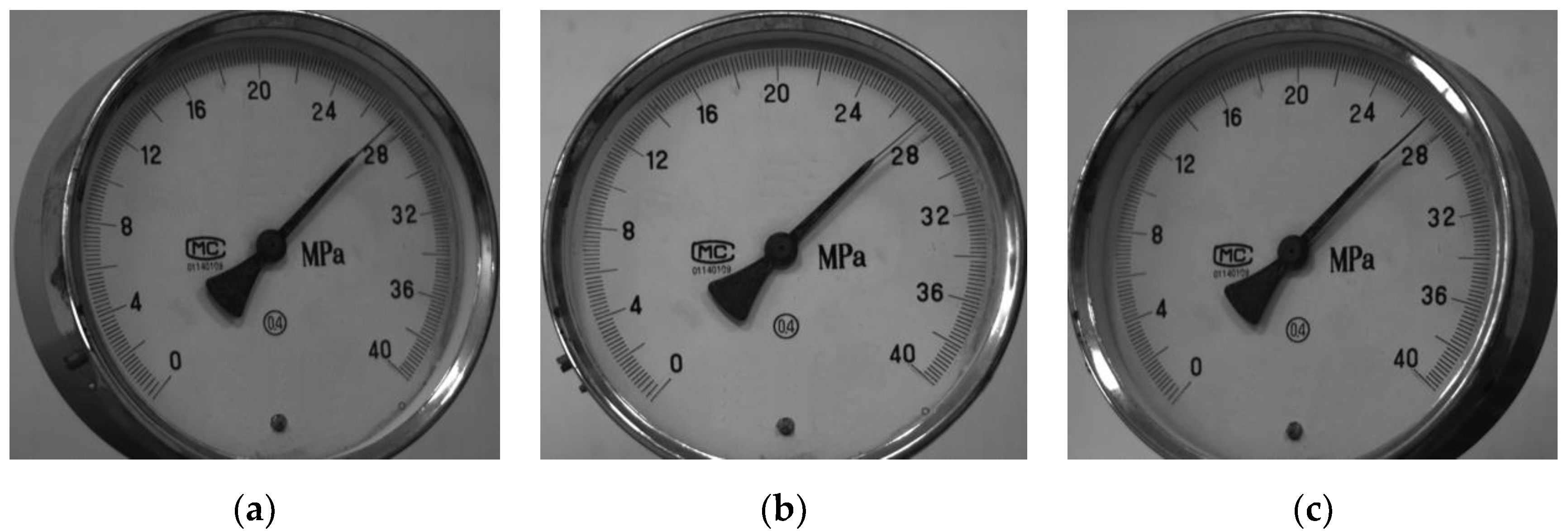
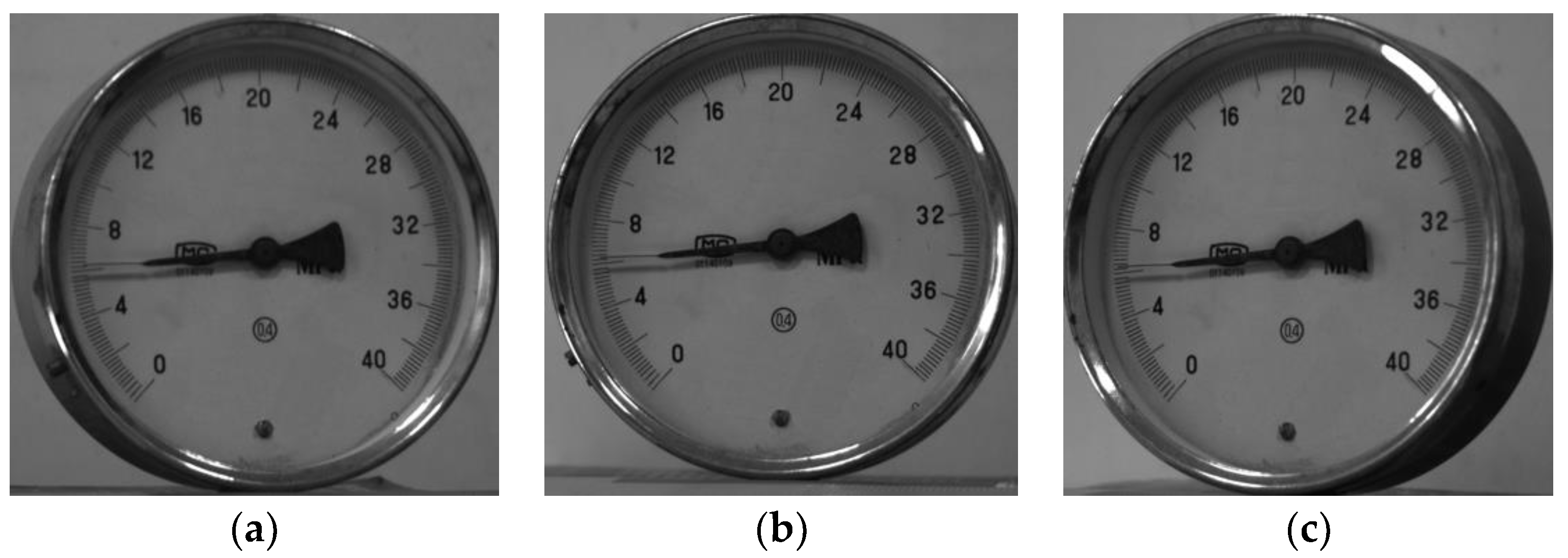
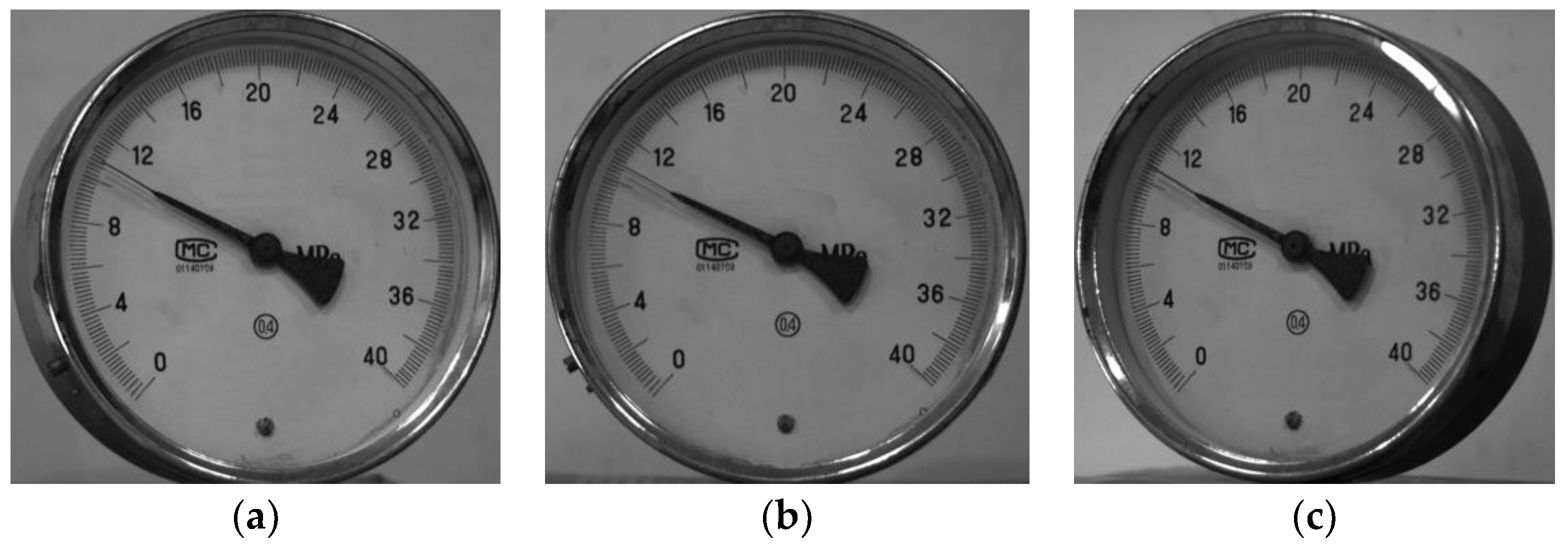
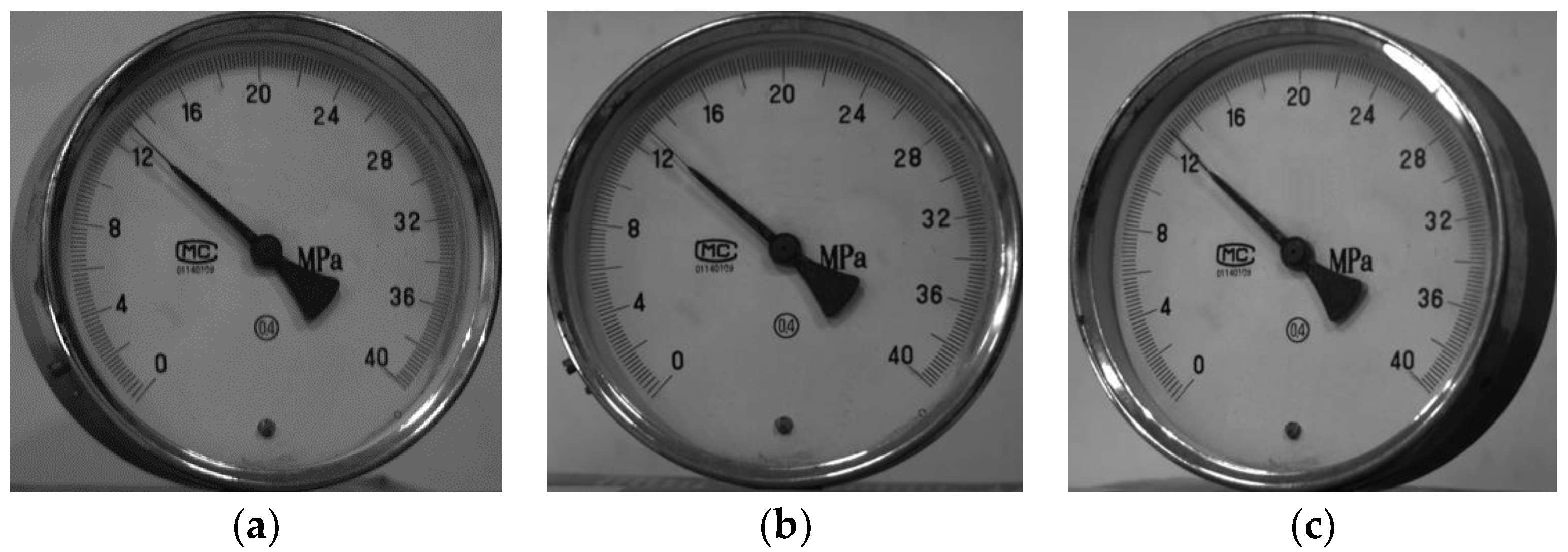
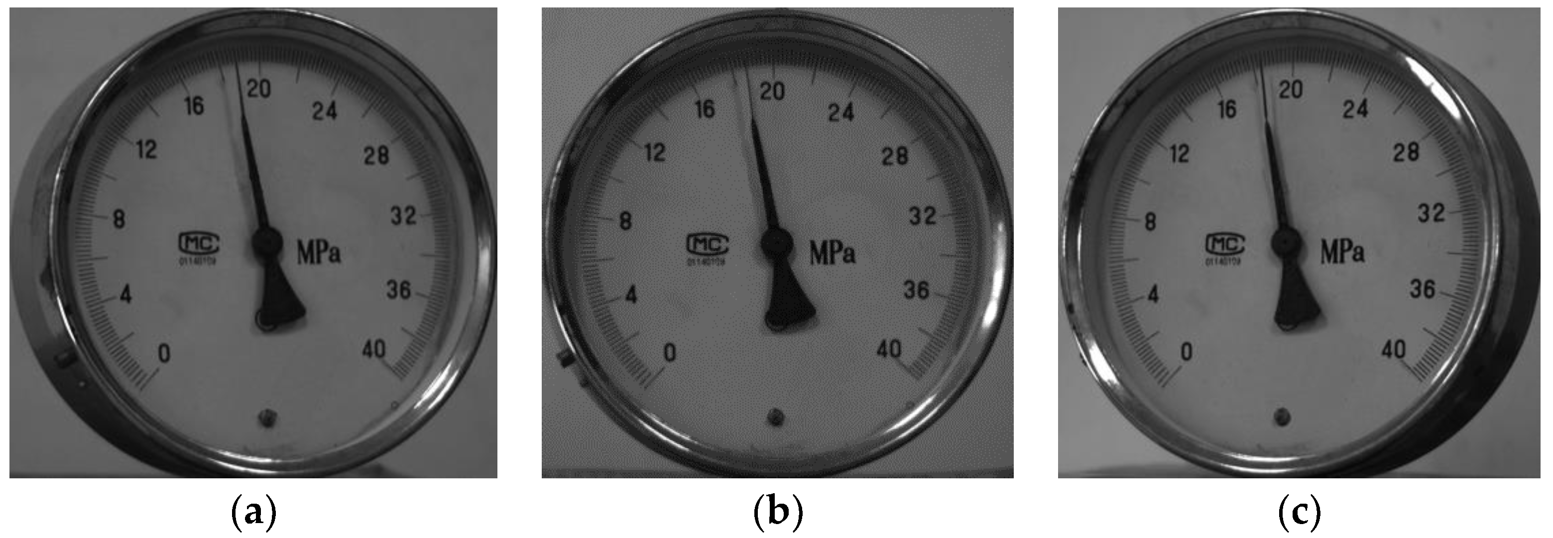
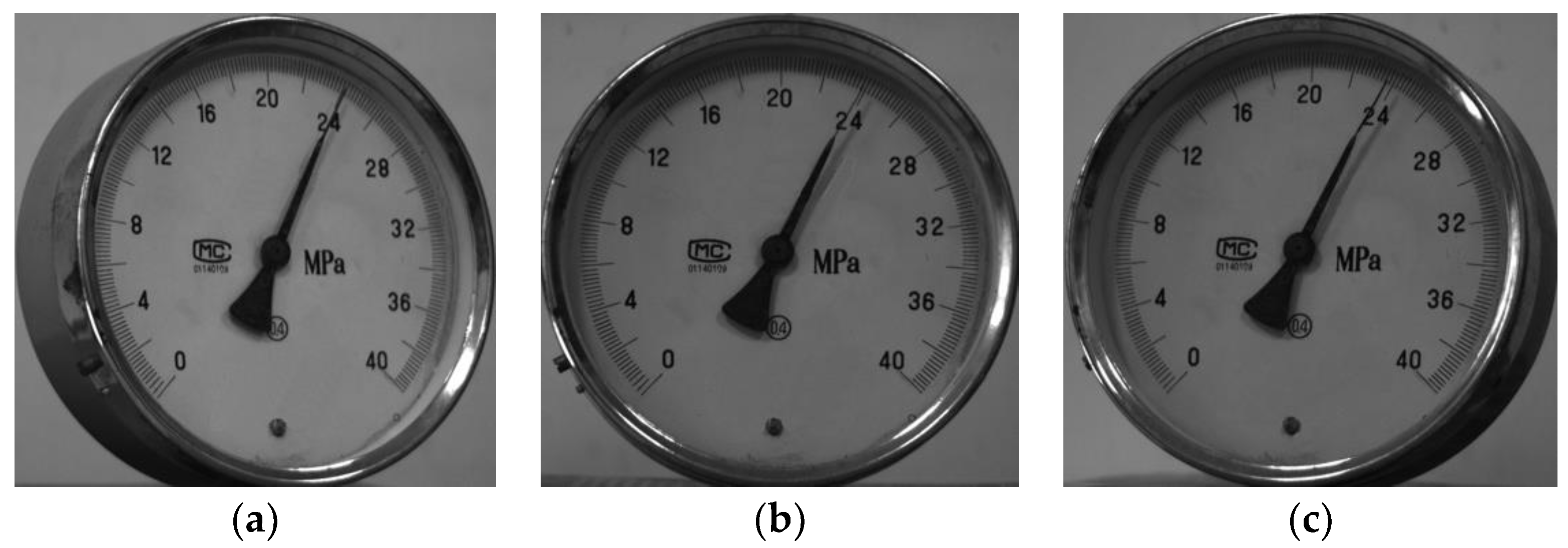
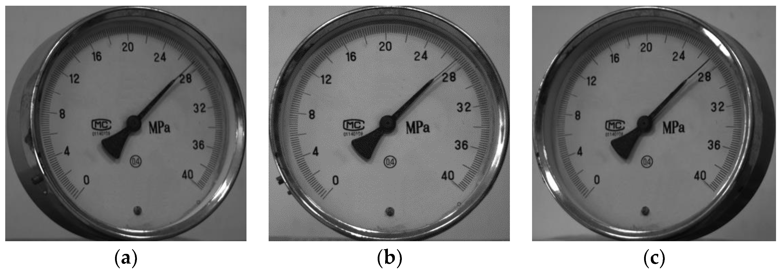
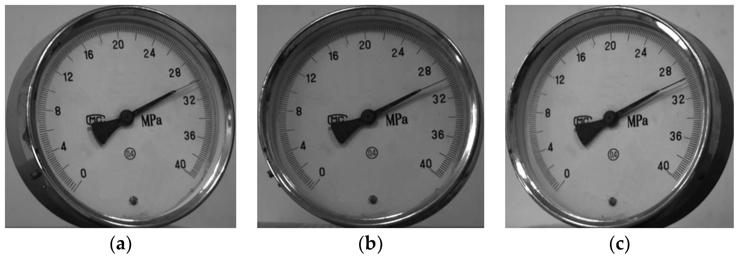
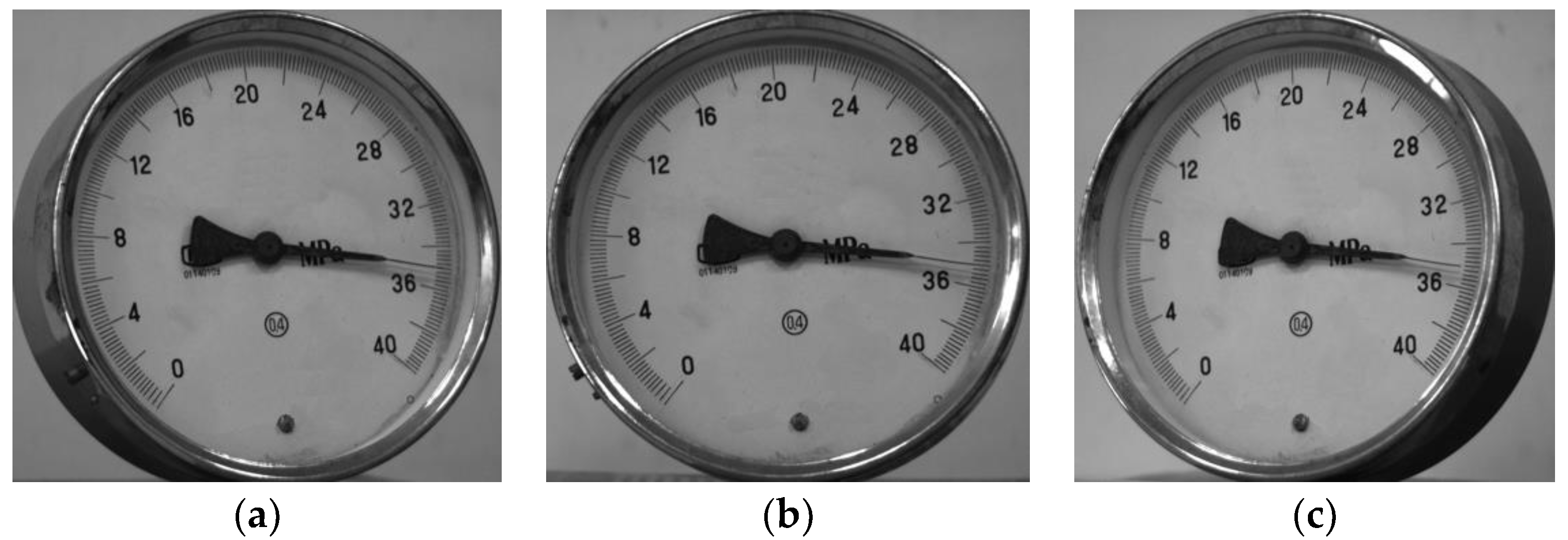
Under the same conditions, the three operators sequentially observed the same location of the pointer and recorded the readings of the pointer meter. Average value of the readings was used as the reference value for assessing the repeatability of the present method. Then, under keeping that the pointer location was the same with the operators observing, images of the pointer meter were taken from three different angles, as shown in Figure 5, and reading of the pointer meter was measured by the present method and the conventional method [25]. In Appendix B, the images of the pointer meter taken from three different angles were given for all the location of the pointer in the measurement.
First, the radius r l and r s from the rotation center to the midpoint of long scales and short scales on the pointer meter were measured, that is r l = 602.5   mm and r s = 584.6   mm respectively. And angle between the zero scale and the maximum scale was measured, that was α = 271.5 
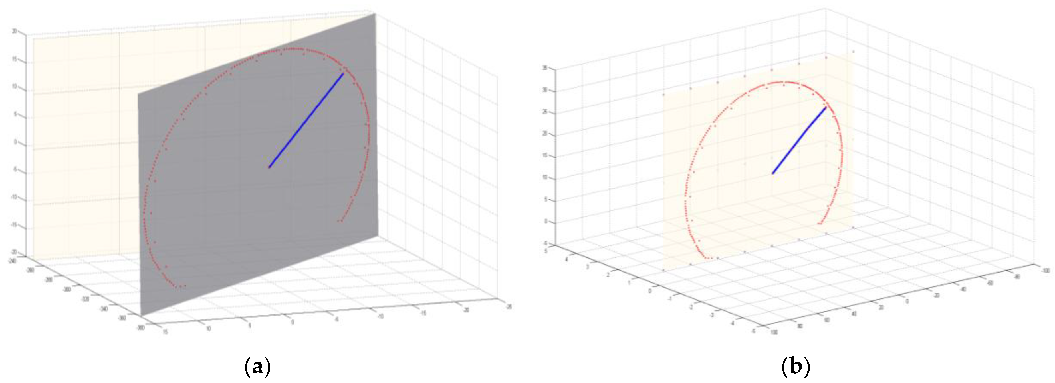
. So, the world coordinates of the midpoints of short scales were obtained based on Equation (1). Second, the pixel coordinates of all the midpoints of scales and critical points (including rotation center and ends of pointer) were detected. After calibration the intrinsic parameters, the extrinsic parameters can be calibrated by the pixel coordinates and world coordinates of midpoints of short scales, as shown in Figure 6a.
The extrinsic parameters were expressed as [ R , T ] = [ 0.7620 0.6469 7.2419 0.6467 0.7626 14.4477 0.0326 0.0070 895.6315 ] . And the world coordinates of midpoints on the short scales were transformed into the camera coordinates by the extrinsic parameters.
Second, normal vector k of the meter surface was calculated by the camera coordinates of three midpoints to obtain the rotation transformation matrix M of the meter image based on Equation (2). The meter image was rotated by the matrix M to make the meter image parallel to the surface of the meter, as shown in Figure 7. Therefore, the coordinates of the critical point on the pointer meter can be corrected in this way, identifying the reading of the pointer meter by Equation (4). The coordinates of the endpoint of the pointer and rotation center in each pose were reported during the measurement in Table 2 and Table 3. After rotating the meter image, changes of the coordinates of the endpoints and rotation center were shown in Table 2 and Table 3.
Then, the readings of the pointer meter were compared with the reference value to calculate absolute errors, as shown in Table 4 and Table 5. Here, f 0 was the reference value; f 1 ( 1 ) , f 1 ( 2 ) , f 1 ( 3 ) respectively represented the results of readings measured by conventional methods in the meter image taken from three angles; f 2 ( 1 ) , f 2 ( 2 ) , f 2 ( 3 ) respectively represented the results of readings measured by proposed methods in the meter image taken from the three angles which kept the same angle as conventional measurement.
The pointer meter used in the experiment was a 0 to 40 MPa pressure gauge with a precision of δ = Δ max 40 × 100 % = 0.4 % , and the pointer meter’s maximum allowable absolute error was Δ max = 0.16   MPa . The range accuracy of the meter reached 2 digits after the decimal point. In order to make the accuracy of the meter recognition algorithm reach the accuracy of the meter range, this paper kept the effective digit to the next digit of the precision. The pixel coordinates of mid-point scales were achieved using the sub-pixel detection method to improve the measurement resolution. In the experiment, the image of the pointer meter was 1292 × 964 pixels captured by a camera. We estimated the arc length l = 8.6 pixel by calculating the distance between center points of two adjacent scales, and the radius of the pointer meter region r = 363.77 pixel can also be calculated. Then, the angle δ = 180 × l π × r = 1.36 was converted from the arc length. And the angle δ v occupied by each pixel was 0.15°. Therefore, the camera’s hardware resolution was 0.15° under this experimental condition which includes strength of illumination and the distance d = 1.5 m between camera and measured meter plane.
As shown in Table 6 and Table 7, the absolute errors Δ f 2 ( 1 ) , Δ f 2 ( 2 ) , Δ f 2 ( 3 ) of the measurement by proposed method were mostly between 1 kPa and 9 kPa. The maximum absolute error 9 kPa still did not exceed the absolute errors Δ f 1 ( 1 ) , Δ f 1 ( 2 ) , Δ f 1 ( 3 ) of measurement by the conventional method. In addition, through the proposed method, the readings of the measured pointer meter in the images taken from three angles had almost no change compared with the reference values. It can be seen from the experimental results that the identification accuracy of the pointer meter calibration system was within the allowable range. Compared with the conventional measurement method, the maximum relative error was Δ f r = 0 . 022 % , which met the measurement requirements.

3.2. Measure Two Pointer Meters

As with measuring one pointer meter, the three operators sequentially observed the same location of the pointer of the meter on the left in the image and recorded the readings under the same conditions. Average value of the readings of the meter on the left in the image was used as the reference value g 0 ( 1 ) . And the three operators sequentially observed again the same location of the pointer of the meter on the right in the image and recorded the readings. Average value of the readings of the meter on the right in the image was used as the reference value g 0 ( 2 ) . The reference values g 0 ( 1 ) and g 0 ( 2 ) were used for assessing the repeatability of the present method.
In order to verify that multiple pointer meters can be measured based on the proposed method, two pointer meters which had the same size and the same range were measured. The actual radius on the pointer meter from the rotation center to the midpoint of long scales and short scales was measured, that was 469 mm and 455 mm respectively. The angle between the zero scale line and the maximum scale line was measured, that was α = 271.8 . Then, the world coordinates of the one of pointer meters’ short scales midpoints in were obtained based on Equation (1).
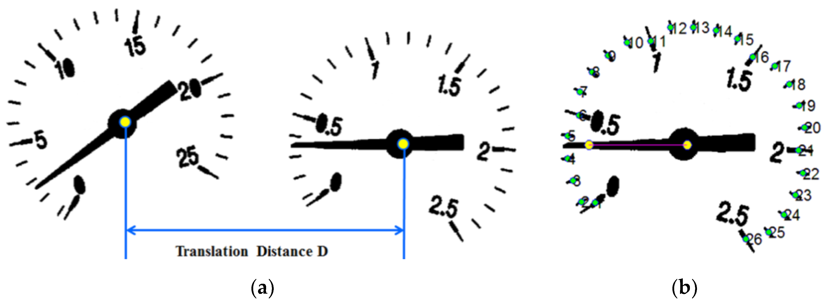
First, the pixel coordinates of all the midpoints of scales and critical points (including rotation center and ends of pointer) of the two pointer meters were detected. The translation distance D between the two pointer meters can be calculated using the distance between rotation centers of the two pointer meters, as shown in Figure 8a. After calibration the intrinsic parameters, the extrinsic parameters can be calibrated by the pixel coordinates and world coordinates of midpoints of short scales of the meter on the left in the image, as shown in Figure 6b. The extrinsic parameters were expressed as [ R , T ] = [ 0.2261 0.9732 0.0416 0.0039 0.0418 0.9991 0.9741 0.2261 0.0056 ] . And the world coordinates of midpoints on the short scales of the meter on the left in the image were transformed into the camera coordinates by the extrinsic parameters.
Second, normal vector k of the meter surface was calculated by the camera coordinates of three midpoints to obtain the rotation transformation matrix M of the meter image based on Equation (2). The meter image was rotated by the matrix M to make the meter image parallel to the surface of the meter. Therefore, the pixel coordinates of the critical point (including the rotation center and the endpoint of the pointer) of the meter on the left in the image can be corrected in this way, identifying the readings of the meter on the left in the image by Equation (4). Through the translation distance D, the reading of the pointer meter on the right in the image can also be detected, as shown in Figure 8b.
During the experiment, the positions of the two pointer meters were changed from zero scale line to maximum scale line, and there were 8 times of measurement in each group. Under keeping that the pointer location same with the operators observing, and reading of the pointer meter is measured by the present method and the conventional method respectively. The readings of the pointer meter were compared with the reference value to calculate absolute errors, as shown in Table 8. Here, the g 0 ( 1 ) and g 0 ( 2 ) were the reference value of the meter on the left and the meter on the right in the image; g 1 ( 1 ) , g 1 ( 2 ) respectively represented the results of readings of two pointer meters measured by conventional methods; g 2 ( 1 ) , g 2 ( 2 ) respectively represented the results of readings of the two pointer meters measured by proposed methods.
As shown in Table 9, the absolute errors Δ g 2 ( 1 ) , Δ g 2 ( 2 ) of the measurement by proposed method were mostly between 1 kPa and 16 kPa. The maximum error of 16 kPa still did not exceed the absolute errors Δ g 1 ( 1 ) , Δ g 1 ( 2 ) of measurement by the traditional method. Comparing with the reference value, the measured values had little change. It can be seen from the experimental results that the identification accuracy of the pointer meter calibration system is within the allowable range. Compared with the conventional measurement method, the maximum relative error is 0.064%, which meets the measurement requirements.
From the results of the experiment, there are still errors in the presented method of recognizing the readings of pointer meter. The main reason is uneven distribution of the scale lines in the pointer meter. The meter scales on the pointer meter are used as the calibration objects to obtain the extrinsic parameters of the meter plane. The error of the extrinsic parameters calibration is caused by the incomplete equal distance between the mid-points of two adjacent scales. In addition, the changes in light intensity and the distance between the camera and the meter plane would vary the quality of the image, which will also results in deviations in the extraction of pixel coordinates of t critical points in the image.

4. Conclusions

A computer vision method for automatically identifying the readings of multiple pointer meters is proposed in this paper. The extrinsic parameters of the meter plane are calibrated by the pixel coordinates and world coordinates of the mid-points of the measured meter scale instead of the traditional calibration pattern. The meter image is made parallel to the surface of the meter by inverse perspective mapping. The mapping is finished by rotation transformation of the meter image, and the rotation transformation matrix is obtained, eliminating the perspective effect of the meter image. The transformed image is measured by the visual detection method to obtain the readings of the pointer meter, correcting the coordinates of the rotation center and the end point of the pointer. From the results of the measurement, the readings of the pointer meter are hardly affected by the non-coplanarity of the imaging and pointer meters.

Author Contributions

Conceptualization, Q.T. and H.B.; methodology, Q.T.; software, H.B. and S.L.; validation, S.L. and J.M.; formal analysis, Q.T.; investigation, J.M.; data curation, H.B.; writing—original draft preparation, H.B. and Q.T.; writing—review and editing, H.B. and Q.T.; visualization, S.L.; supervision, J.M.

Funding

This research received no external funding.

Conflicts of Interest

The authors declare no conflict of interest.

Appendix A

The imaging model of the camera included the world coordinate system (OiWXiWYiWZiW), the camera coordinate system (OCXCYCZC), the image coordinate system (Oxy), and the pixel coordinate system (Opuv), as shown in Figure A1.
Figure A1. The imaging model of the camera.
Applsci 09 03729 g0a1
Mapping from world coordinate system to pixel coordinate system can be represented in Table A1, where R is the rotation matrix; T is the translation vector; k 1 ( H ) , k 2 ( H ) , p 1 ( H ) , p 2 ( H ) are the coefficients of the radial and tangential distortions; A = [ α γ u 0 0 β v 0 0 0 1 ] is the camera intrinsic parameters; and ZW = 0 in the model. The intrinsic parameters could be obtained by optimizing the object function, which is established by minimizing the distance between the calculated pixel coordinates and the actual pixel of the corner points on the calibration board. This function is solved by the Levenberg Marquardt algorithm.
Table A1. Coordinate transformation camera model.
TransformationFormulas
From world coordinate system to camera coordinate system [ X C Y C Z C ] = R [ X W Y W 1 ] + T     (1)
From camera coordinate system to image coordinate system [ x u y u ] = 1 Z c [ X c Y c ]     (2)
Introducing the distortion model, where, r2 = x2d + y2d, [ x u y u ] = ( 1 + k 1 ( H ) r 2 + k 2 ( H ) r 4 ) [ x d y d ] + [ 2 p 1 ( H ) x d y d + p 2 ( H ) ( r 2 + 2 x d 2 ) p 1 ( H ) ( r 2 + 2 y d 2 ) + 2 p 2 ( H ) x d y d ] (3)
From image coordinate system to pixel coordinate system [ u v 1 ] = [ α γ C x 0 β C y 0 0 1 ] [ x d y d 1 ]     (4)

Appendix B

Figure A2. The meter image taken by camera from three angles when the reading of the pointer meter is 6.2; (a) the camera at position 1; (b) the camera at position 2; (c) the camera at position 3.
Applsci 09 03729 g0a2
Figure A3. The meter image taken by camera from three angles when the reading of the pointer meter is 10.7; (a) the camera at position 1; (b) the camera at position 2; (c) the camera at position 3.
Applsci 09 03729 g0a3
Figure A4. The meter image taken by camera from three angles when the reading of the pointer meter is 12.9; (a) the camera at position 1; (b) the camera at position 2; (c) the camera at position 3.
Applsci 09 03729 g0a4
Figure A5. The meter image taken by camera from three angles when the reading of the pointer meter is 18.6; (a) the camera at position 1; (b) the camera at position 2; (c) the camera at position 3.
Applsci 09 03729 g0a5
Figure A6. The meter image taken by camera from three angles when the reading of the pointer meter is 23.9; (a) the camera at position 1; (b) the camera at position 2; (c) the camera at position 3.
Applsci 09 03729 g0a6
Figure A7. The meter image taken by camera from three angles when the reading of the pointer meter is 26.9; (a) the camera at position 1; (b) the camera at position 2; (c) the camera at position 3.
Applsci 09 03729 g0a7
Figure A8. The meter image taken by camera from three angles when the reading of the pointer meter is 30.2; (a) the camera at position 1; (b) the camera at position 2; (c) the camera at position 3.
Applsci 09 03729 g0a8
Figure A9. The meter image taken by camera from three angles when the reading of the pointer meter is 35.1; (a) the camera at position 1; (b) the camera at position 2; (c) the camera at position 3.
Applsci 09 03729 g0a9

Appendix C

Table A2. Description of Symbols in the paper.
SymbolDefinitionThe Number of Equation/Section
( X W i , Y W i , Z W i ) T the world coordinates of midpoint of scaleEquation (1)
r s the radius of the pointer meterEquation (1)
γ the center angle between neighbors two scalesEquation (1)
( u , v ) T the sub-pixel coordinates of midpoint of scaleSection 2.1
[ R , T ] the extrinsic parametersSection 2.1
( X C i , Y C i , Z C i ) T the camera coordinates of midpoint of scaleSection 2.1
k = [ k x , k y , k z ] the normal vector of the meter surfaceSection 2.1
θ the rotation angleSection 2.1
M the rotation transformation matrixEquation (2)
( X i , Y i , Z i ) T the camera coordinates of points in the meter imageEquation (3)
( x i , y i , z i ) T the camera coordinates of the midpoints in the transformed meter imageEquation (3)
p 1 ( x 1 , y 1 ) the coordinate of midpoint of zero-scale lineEquation (4)
p M ( x M , y M ) the coordinate of midpoint of maximum-scale lineEquation (4)
c ( x c , y c ) the coordinate of rotation centerEquation (4)
e ( x e , y e ) the coordinate of endpoint of the pointerEquation (4)
α the angle between zero scale line and the maximum scale lineEquation (4)
β the angle between the detected pointer and zero scale lineEquation (4)

References

  1. Matić, T.; Aleksi, I.; Hocenski, Ž.; Kraus, D. Real-time biscuit tile image segmentation method based on edge detection. ISA Trans. 2018, 76, 246–254. [Google Scholar] [CrossRef]
  2. Sun, Q.; Liang, F.; Wang, F.; Cong, H.; Li, Q.; Yan, J. investigation on the geometrical characteristics of secondary arc by image edge detection. IEEE Trans. Plasma Sci. 2018, 46, 2016–2025. [Google Scholar] [CrossRef]
  3. Gaurav, K.; Ghanekar, U. Image steganography based on Canny edge detection, dilation operator and hybrid coding. J. Inf. Secur. Appl. 2018, 41, 41–54. [Google Scholar] [CrossRef]
  4. Abed, S.E.; Ali, M.H.; Al-Shayeji, M. An adaptive edge detection operator for noisy images based on a total variation approach restoration. Comput. Syst. Sci. Eng. 2017, 32, 199–211. [Google Scholar]
  5. Sablatnig, R.; Kropatsch, W.G. Automatic reading of analog display instruments. Pattern Recognit. 1994, 1, 794–797. [Google Scholar]
  6. Alegria, E.C.; Serra, A.C. Automatic calibration of analog and digital measuring instruments using computer vision. IEEE Trans. Instrum. Meas. 2000, 49, 94–99. [Google Scholar] [CrossRef]
  7. Zhao, S.; Li, B.; Yuan, J.; Cui, G. Research on remote meter automatic reading based on computer vision. In Proceedings of the IEEE/PES Transmission and Distribution Conference & Exhibition: Asia and Pacific Dalian, Dalian, China, 18 August 2005; pp. 1–4. [Google Scholar]
  8. Feng, H.P.; Zhao, J. Application research of computer vision in the auto-calibration of dial gauges. In Proceedings of the 2008 International Conference on Computer Science and Software Engineering, Wuhan, China, 12–14 December 2008; pp. 845–848. [Google Scholar]
  9. Zhang, Z.; Li, Y.; Yuan, W. Research on pointer location of multi-pointer meter. In Proceedings of the IEEE International Conference on Automation and Logistics, Shenyang, China, 5–7 August 2009; pp. 911–914. [Google Scholar]
  10. Behaine, C.A.R.; Scharcanski, J. Remote visual monitoring of analogue meter displays using deformable models. IET Sci. Meas. Technol. 2014, 8, 228–235. [Google Scholar] [CrossRef]
  11. Ma, Y.; Jiang, Q. A robust and high-precision automatic reading algorithm of pointer meters based on machine vision. Meas. Sci. Technol. 2018, 30, 015401. [Google Scholar] [CrossRef]
  12. Hemming, B.; Lehto, H. Calibration of dial indicators using machine vision. Meas. Sci. Technol. 2002, 13, 45–49. [Google Scholar] [CrossRef]
  13. Hemming, B.; Fagerlund, A.; Lassila, A. High-accuracy automatic machine vision based calibration of micrometers. Meas. Sci. Technol. 2007, 18, 1655–1660. [Google Scholar] [Green Version]
  14. De Lima, D.A.; Pereira, G.A.S.; de Vasconcelos, F.H. A Computer vision system to read meter displays. In Proceedings of the 16th IMEKO TC4 Symposium Exploring New Frontiers of Instrumentation and Methods for Electrical and Electronic Measurements, Florence, Italy, 22–24 September 2008; pp. 1–5. [Google Scholar]
  15. Vázquez-Fernández, E.; Dacal-Nieto, A.; González-Jorge, H.; Martín, F.; Formella, A.; Alvarez-Valado, V. A machine vision system for the calibration of digital thermometers. Meas. Sci. Technol. 2009, 20, 065106. [Google Scholar] [CrossRef]
  16. Belan, P.A.; Araujo, S.A.; Librantz, A.F.H. Segmentation-free approaches of computer vision for automatic calibration of digital and analog instruments. Measurement 2013, 46, 177–184. [Google Scholar] [CrossRef]
  17. Yang, B.; Lin, G.; Zhang, W. Auto-recognition method for point-type meter based on binocular vision. JCP 2014, 9, 787–793. [Google Scholar]
  18. Cui, Y.; Luo, W.; Fan, Q.; Peng, Q.; Cai, Y.; Yao, Y.; Xu, C. Design and implementation of pointer-type multi meters intelligent recognition device based on arm platform. J. Phys. Conf. Ser. 2018, 960, 012036. [Google Scholar] [CrossRef]
  19. Zhang, Z. Flexible camera calibration by viewing a plane from unknown orientations. In Proceedings of the IEEE International Conference on Computer Vision, Kerkyra, Greece, 20–27 September 1999; pp. 666–673. [Google Scholar]
  20. Zhou, F.; Zhao, J.; Ye, T.; Chen, L. Fast star centroid extraction algorithm with sub-pixel accuracy based on FPGA. J. Real Time Image Proc. 2016, 12, 613–622. [Google Scholar] [CrossRef]
  21. Yoneyama, S.; Kikuta, H.; Kitagawa, A.; Kitamura, K. Lens distortion correction for digital image correlation by measuring rigid body displacement. Opt. Eng. 2006, 45, 023602. [Google Scholar] [CrossRef]
  22. Tancharoen, D.; Jitapunkul, S.; Chompun, S. Spatial segmentation based on modified morphological tools. In Proceedings of the Information Technology: Coding and Computing International Conference, Las Vegas, NV, USA, 2–4 April 2001; 478–482; pp. 478–482. [Google Scholar]
  23. Fitzgibbon, A.; Pilu, M.; Fisher, R.B. Direct least square fitting of ellipses. IEEE Trans. Pattern Anal. Mach. Intell. 1999, 21, 476–480. [Google Scholar] [CrossRef] [Green Version]
  24. Hough, P.V. Method and Means for Recognizing Complex Patterns. U.S. Patent No. 3069654, 18 December 1962. [Google Scholar]
  25. Aydogmus, O.; Talu, M.F. A vision-based measurement installation for programmable logic controllers. Measurement 2012, 45, 1098–1104. [Google Scholar] [CrossRef]
Figure 1. The distance between the each pointer meter and the camera is the same; (a) the pointer meter plane is facing the camera at an angle; (b) the pointer meter plane is facing the camera.
Applsci 09 03729 g001
Figure 2. The different steps of measurement the readings of the pointer meter.
Applsci 09 03729 g002
Figure 3. Result of the detected the end point e ( x e , y e ) of pointer, the rotation center c ( x c , y c ) and all the midpoints of scales in the pointer meter.
Applsci 09 03729 g003
Figure 4. (a) Measured pointer meter with radius of 620 mm; (b) measured pointer meters with a radius of 406 mm.
Applsci 09 03729 g004
Figure 5. Measured pointer meter captured from three different angles; (a) the camera at position 1; (b) the camera at position 2; (c) the camera at position 3.
Applsci 09 03729 g005
Figure 6. (a) Result of all the midpoints of short scales in the pointer meter with radius of 620 mm; (b) result of all the midpoints of short scales of the meter on the left in the image with radius of 406 mm.
Applsci 09 03729 g006
Figure 7. (a) Illustration of pointer meter plane before Reverse Projection; (b) illustration of pointer meter plane after Reverse Projection.
Applsci 09 03729 g007
Figure 8. (a) Translation distance between two pointer meters; (b) result of critical points of the meter on the right in the image.
Applsci 09 03729 g008
Table 1. Main experimental devices.
No.NameTypePerformance
1CCD cameraJAI CCD cameraResolution: 1376 × 1024
2LensM0814-MPFocal length: 25 mm
3Model planeNANO CBC 75MM-2.0Precision of grid: 1 μm
4BacklightCCS LFL-200Color: red
5Pointer meter1Pressure gaugeRange: 0–40 MPa; Radius: 650 mm
6Pointer meter2Oxygen pressure gaugeRange: 0–25 MPa; Radius: 400 mm
Range: 0–2.5 MPa; Radius: 400 mm
Table 2. Comparison for the pixel coordinates of pointer endpoint.
No.Reference Values f 0 (MPa)Coordinates of Pointer Endpoint e 1 ( x e 1 , y e 1 ) Coordinates of Pointer Endpoint after Reverse Projection e ( x e , y e )
16.2(373.7191, 534.5052)(249.1572, 526.5000)
210.7(432.0370, 310.4386)(298.5000, 301.3333)
312.9(510.9333, 203.0400)(382.0533, 191.0400)
418.6(753.3243, 65.5000)(653.6667, 52.0270)
523.9(1010.6000, 115.6711)(929.1842, 104.5000)
626.9(1095.8000, 176.6250)(1020.5000, 170.4412)
730.2(1211.5000, 373.8158)(1151.5000, 359.5834)
835.1(1206.5000, 645.8571)(1164.5000, 627.8919)
Table 3. Comparison for the pixel coordinates of rotation center.
No.Reference Values f 0 (MPa) Coordinates of Rotation Center c 1 ( x c 1 , y c 1 ) Coordinates of Rotation Center after Reverse Projection c ( x c , y c )
16.2(757.5000, 522.1006)(757.2410, 522.1089)
210.7(758.1498, 525.2314)(758.3021, 525.2321)
312.9(757.9612, 524.9675)(757.9635, 524.5019)
418.6(757.2554, 522.2103)(757.0241, 522.5742)
523.9(758.5000, 525.3600)(757.9266, 525.0143)
626.9(758.5000, 524.8661)(758.2169, 525.2106)
730.2(757.1893, 523. 6752)(756.6355, 524. 8814)
835.1(757.5000, 524.5000)(757.8577, 524.5.1983)
Table 4. Comparison of the results of readings measured by conventional methods in the meter image taken from three angles.
No.Reference Values
f 0 (MPa)
Position 1
f 1 ( 1 ) (MPa)
Position 2
f 1 ( 2 ) (MPa)
Position 3
f 1 ( 3 ) (MPa)
16.26.0596.3426.301
210.710.54210.79610.859
312.912.75312.80613.043
418.618.46918.50718.748
523.924.03923.77123.752
626.927.02127.05726.753
730.230.35830.30630.059
835.134.96635.00235.254
Table 5. Comparison of the results of readings measured by proposed methods in the meter image taken from three angles.
No.Reference Values
f 0 (MPa)
Position 1
f 2 ( 1 ) (MPa)
Position 2
f 2 ( 2 ) (MPa)
Position 3
f 2 ( 3 ) (MPa)
16.26.1986.1996.206
210.710.69910.70110.703
312.912.89712.90212.898
418.618.60118.59618.605
523.923.89723.89123.902
626.926.89926.90126.901
730.230.20230.20130.198
835.135.10135.09935.098
Table 6. Measurement absolute errors by the conventional method.
No.Absolute Error of Position 1
Δ f 1 ( 1 ) = | f 1 ( 1 ) f 0 | (kPa)
Absolute Error of Position 2
Δ f 1 ( 2 ) = | f 1 ( 2 ) f 0 | (kPa)
Absolute Error of Position 3
Δ f 1 ( 3 ) = | f 1 ( 3 ) f 0 | (kPa)
1141142101
215896159
314794143
413193148
5139129148
6121157147
7158106141
814098154
Table 7. Measurement absolute errors by the proposed method.
No.Absolute Error of Position 1
Δ f 2 ( 1 ) = | f 2 ( 1 ) f 0 | (kPa)
Absolute Error of Position 2
Δ f 2 ( 2 ) = | f 2 ( 2 ) f 0 | (kPa)
Absolute Error of Position 3
Δ f 2 ( 3 ) = | f 2 ( 3 ) f 0 | (kPa)
1216
2113
3322
4145
5392
6111
7212
8112
Table 8. Measurement readings of two pointer meters by two methods.
No.Reference Values 1
/Reference Values 2
g 0 ( 1 ) / g 0 ( 2 ) (MPa)
Traditional Measurement Results 1
/Traditional Measurement Results 2
g 1 ( 1 ) / g 1 ( 2 ) (MPa)
Measurement Results 1
/Measurement Results 2
g 2 ( 1 ) / g 2 ( 2 ) (MPa)
11.3/0.31.101/0.3121.238/0.325
25.6/0.86.098/0.7125.610/0.768
38.1/0.98.791/0.8348.126/0.920
412.8/1.213.013/1.14912.765/1.240
516.7/1.516.847/1.46716.654/1.476
619.1/1.619.863/1.61119.111/1.638
722.7/2.022.910/1.93522.670/1.981
824.8/2.224.996/2.24624.815/2.248
Table 9. Measurement absolute errors of two pointer meters for two methods.
No.Absolute Error Δ f 1 ( 1 ) /Absolute Error Δ f 1 ( 2 ) of Conventional Measurement
Δ g 1 ( 1 ) = | g 1 ( 1 ) g 0 ( 1 ) | / Δ g 1 ( 2 ) = | g 1 ( 1 ) g 0 ( 2 ) | (kPa)
Absolute Error Δ f 2 ( 1 ) /Absolute Error Δ f 2 ( 2 ) of Measurement
Δ g 2 ( 1 ) = | g 2 ( 1 ) g 0 ( 1 ) | / Δ g 2 ( 2 ) = | g 2 ( 1 ) g 0 ( 2 ) | (kPa)
1199/1212/5
2489/8810/2
3691/666/1
4213/515/1
5147/3316/4
6763/1111/2
7210/652/9
8166/4610/2

