Article

UAV-Based Air Pollutant Source Localization Using Combined Metaheuristic and Probabilistic Methods †

by
Noe Yungaicela-Naula
1,
Luis E. Garza-Castañon
1,*,
Youmin Zhang
2 and
Luis I. Minchala-Avila
3
1
School of Engineering and Science, Tecnologico de Monterrey, Eugenio Garza Sada 2501, Monterrey 64849, Mexico
2
Department of Mechanical, Industrial and Aerospace Engineering, Concordia University, 1455 de Maisonneuve Blvd., Montreal, QC H3G 1M8, Canada
3
Department of Electronic and Telecommunication Engineering, Universidad de Cuenca, Av. 12 de Abril y Agustín Cueva, Cuenca 0101168, Ecuador
*
Author to whom correspondence should be addressed.
This paper is an extended version published in the 2018 International Conference on Unmanned Aircraft Systems (ICUAS), Dallas, TX, USA, 12–15 June 2018.
Appl. Sci. 2019, 9(18), 3712; https://doi.org/10.3390/app9183712
Submission received: 3 August 2019 / Revised: 20 August 2019 / Accepted: 29 August 2019 / Published: 6 September 2019
(This article belongs to the Special Issue Autonomous Micro Aerial Vehicles: Methods and Applications)

Abstract

:
Air pollution is one of the greatest risks for the health of people. In recent years, platforms based on Unmanned Aerial Vehicles (UAVs) for the monitoring of pollution in the air have been studied to deal with this problem, due to several advantages, such as low-costs, security, multitask and ease of deployment. However, due to the limitations in the flying time of the UAVs, these platforms could perform monitoring tasks poorly if the mission is not executed with an adequate strategy and algorithm. Their application can be improved if the UAVs have the ability to perform autonomous monitoring of the areas with a high concentration of the pollutant, or even to locate the pollutant source. This work proposes an algorithm to locate an air pollutant’s source by using a UAV. The algorithm has two components: (i) a metaheuristic technique is used to trace the increasing gradient of the pollutant concentration, and (ii) a probabilistic component complements the method by concentrating the search in the most promising areas in the targeted environment. The metaheuristic technique has been selected from a simulation-based comparative analysis between some classical techniques. The probabilistic component uses the Bayesian methodology to build and update a probability map of the pollutant source location, with each new sensor information available, while the UAV navigates in the environment. The proposed solution was tested experimentally with a real quadrotor navigating in a virtual polluted environment. The results show the effectiveness and robustness of the algorithm.

1. Introduction

Air pollution is one of the major factors affecting the health of people, leading to one in nine deaths worldwide [1]. Short-term and long-term health risks, attributed to exposure to air pollution, are very critical, for example, breathing problems, cardiovascular diseases and lung cancer [2,3,4,5].
Platforms for monitoring air pollution have played an important role in dealing with the pollution problem, where the Unmanned Aerial Vehicles (UAVs) appear to be one of the most disruptive tools for air pollutant monitoring applications [6,7,8,9,10,11], showing great advantages with respect to common methods like terrain stations or satellite imaging. These advantages include high spatial resolution, low cost, security, flexibility, multitasking and ease of deployment [12].
The UAV-based platforms are particularly useful due to their ability to monitor specific areas that could be inaccessible or hazardous for humans, such as congested industrial buildings where the pollutant release cannot be measured at ground levels.
Since the air pollutant monitoring using UAVs could be ineffective with an arbitrary exploration of the spaces in the polluted environment, an algorithm, which guides the navigation of the vehicle using online and historical measurements, could be a very useful tool. The location of the pollutant source could be estimated, if the monitoring is concentrated in the most critical areas [13,14,15,16]. We require an algorithm that, in the first place, detects the plume of the pollutant and then concentrates the exploration in the most promising areas, where the UAV has estimated the source could be, using online and historical measurements.
Release of pollutants into the atmosphere has several consequences for potentially many people living in the proximity of its source. Air pollution does not affect only urban areas but also rural. In urban areas, traditional methods of air pollution monitoring (fixed monitoring stations) are being replaced with mobile crowdsensing sensors that are small enough to be carried around by users, or installed in different vehicles [17]. However, this technique is not feasible for rural environments, since the traffic of people and vehicles is scarce. This makes the use of the UAV to locate the air pollutant source important, given its advantage of effectiveness and being able to reach poorly accessible areas [18].
Correct application of the protective measures requires the quick location of the source. However, the localization of the air pollutant concentration using a UAV is challenging, since the environment is very complex. Most of the time, the search region is very large and the effectiveness in locating the source depends not only on the motion of the UAV but also on the unknown and time varying pollutant distribution.
The problem of the UAV-based pollutant source identification depends on two steps [19]:
  • The air pollutant plume localization and
  • The tracing of the pollutant plume towards the source.
The pollutant plume localization implies that the UAV navigates in the targeted environment without useful information about the contaminant levels. A suitable approach could be to perform a deterministic planned navigation in the environment until finding the air pollutant plume. However, it becomes unfeasible in environments with an area much longer that the propagation of the plume, and the limited autonomy of the UAV.
Once the plume is located, the UAV will be able to trace it towards the positions with the highest concentration of the pollutant. Some UAV-based solutions for pollutant plume tracing have been studied that are based mainly on gradient algorithms [13,20]. These algorithms require at least two spatially separated measurements, which are often obtained by using multiple sensors on-board the vehicle or by using multiple measurements separated in time and space with a single sensor.
The gradient-based techniques for plume tracing could be ineffective in a turbulent environment given the too coarse sampling performed by the UAV, relative to the spatial and temporal rates of change in the environment. In addition, some proposed strategies are based on the behavior used by insects or bacteria for foraging or pheromone tracing [21,22], hence the naming of these algorithms as bio-inspired [23,24]. However for biological entities (e.g., moths), the strategy of plume tracing may not be based on olfactory sensor alone, but could be aided by vision, sight, auditory, and/or tactile cues.
This work proposes a metaheuristic algorithm for pollutant source localization using a UAV that combines the gradient-based strategy and a probabilistic method. The gradient-based component is used to trace the plume of the pollutant, while the probabilistic component helps to find the pollutant plume, concentrating the efforts on searching areas with a higher probability of finding the source location. The gradient-based component is a metaheuristic method that has been selected from a simulation-based comparative analysis between some classical techniques. The probabilistic component is based on the work presented in Reference [25], which uses the Bayesian method to build and update a probability map of the pollutant source location, with each new sensor information available while the UAV navigates in the environment.
To test the proposed algorithm, the polluted environment was simulated using a model of particle distribution including turbulence for wind effects. The experimental tests were performed using a real quadrotor which added constraints related to movements and pollutant sensor measurements. The results showed that the UAV was able to find the pollutant plume and trace it towards the source location, even with high variation of the environment and movement constraints of the UAV.
The remaining content of this work is organized as follows. Section 2 describes the pollutant distribution model that is used in the comparative analysis of the metaheuristic algorithms to trace pollutant concentrations and to test the proposed solution of pollutant source localization. Section 3 presents the approach proposed to solve the pollutant source localization. Section 4 presents the comparative analysis of classical metaheuristics to trace the plume of pollutant. Section 5 presents the design of the algorithm to localize the pollutant source, using the metaheuristics selected in the comparative analysis and including the probabilistic strategy. Section 6 presents the results of the experimental test. Finally, the conclusions are drawn in Section 7.

2. Pollutant Distribution Model

The pollutant distribution used in this research is based on the model of the particles diffusion presented in References [26,27], which is based on two assumptions:
  • Conservation of numbers of particles; and
  • The relation between the flux and the density.
Let ψ ( X , t ) denote the particle density of the pollutant at time t and position X = ( x , y , z ) ϵ R 3 . The first condition is given by the following equation:
ψ t + · Γ = s
where Γ ( X , t ) is the pollutant flux and s ( X , t ) is the source function.
The second condition is represented by the components of the flux Γ : diffusion and advection. Diffusion is due to turbulence mixing of particles well modeled under the Fick’s Law:
Γ D = D ψ x
where D : = ( D x , D y , D z ) is the diffusion coefficient.
The advection component is the result of wind components, given by a linear equation:
Γ A = ψ u
where u ( t ) = ( u x ( t ) , u y ( t ) , u z ( t ) ) is the wind velocity vector.
Altogether, the complete model of pollutant is given as:
ψ t + · ( ψ u ) = · ( D ψ ) + s
where D is the diagonal matrix D : = d i a g ( D x , D y , D z ) .
Boundary conditions consider ( x , y , z ) as open dimensions and z = 0 represents the ground, where depositions of pollutant take place, described with the boundary condition:
u s e t ψ D z ψ t = W d e p ψ
where u s e t is the settling velocity for particles, due to gravity and W d e p is the deposition coefficient that models the total flux of particles penetrating in the ground.
Noise components, of two natures, were included in the environment. First, the stochastic behavior of real environment particle concentration is modeled by adding noise as a Gaussian distribution component N ( X , t ) for each point X at time t. The second noise component is given as puffs of pollutant formed by combinations of discrete releasings [28] from multiple sources, close to the targeted environment.

3. Solution Approach

The proposed solution for the UAV-based source localization assumes the following conditions:
  • The targeted environment is limited to a rectangular area in the horizontal space;
  • There is only one source releasing the pollutant;
  • The UAV starts the mission in an arbitrary position on the targeted environment, without information of the plume of pollutant;
  • The UAV has one sensor for the pollutant measurements;
  • It is possible to estimate the vector of the winds in the horizontal plane;
  • The variations of the winds do not affect considerably the control of positioning (navigation) of the UAV;
  • The flying time of the vehicle and the capacity of memory and processing onboard of the vehicle are limited.
Critical features to be considered in the design of the algorithm for the source localization are:
  • The algorithm generates waypoints to guide the UAV towards the pollutant source location;
  • Minimal distances among the waypoints generated by the algorithm are required, hereafter called waypoints resolution. This property will help the UAV to use some strategy of path planning and trajectory planning, to navigate among the waypoints, when the environment has obstacles. Also, as the conventional GPS devices present low resolution, the UAV outdoor navigation could be difficult if the waypoints generated by the algorithm are very close between them; and
  • The precise localization of the source could turn unfeasible in many times, or even the mission can fail in reaching the pollutant plume. Despite this fact, given the captured pollutant and wind information, the system must be able to provide the most probable areas of location of the source.
Measurements of air pollutants are imprecise and depend on sensor quality. The strategy here presented uses these measurements in two approaches—the raw measurement of the sensor, which is the measurement of the pollutant captured by the sensor, and the binary information of the sensor, that is, the raw sensor data are processed to get detection or non-detection information. The two approaches are processed in parallel, making the algorithm more robust.
To get binary information, which will be used by the probabilistic component, the air pollution measurement is processed to define whether it is a detection or non-detection of the pollutant. In our simulated environment, we set a fixed threshold—a value of the pollutant measurement higher than the threshold is a detection, and a value under the threshold is a non-detection. Also, in a real environment, to determine if a measurement is a detection or is not, the measurement scale of the sensor must be considered.
The proposed approach combines two strategies; first, the metaheuristic technique helps to trace the plume concentration towards the source, using the recent and instantaneous raw information of the sensor. The second component is the probabilistic one, which allows our strategy to find the pollutant plume and helps the metaheuristic technique to concentrate the search in areas where the source is probably located. This component uses the binary historical information of the sensor and the wind effects to create and update a probabilistic map of the source localization in the targeted environment.

4. Plume Tracing Algorithm

Since the pollutant distribution could be considered as a variant function in space and time, where the source represents the maximum of the function, many optimization algorithms can be adopted to locate the maximum of the function. This research proposes the use of the metaheuristic approach.
Metaheuristic methods perform an interaction between local improvement procedures and higher-level strategies to create a process capable of escaping from local optimum, while carrying out a robust search of the solution space [29].
The classical metaheuristic techniques can be classified in population-based and trajectory-based approaches. Population-based approaches, such as the genetic algorithms, ant colony, particle swarm optimization, among others, use multiple agents to deal with the optimization problem. On the other hand, trajectory-based strategies, such as simulated annealing and Tabu search, use a single agent which evolves during the algorithm execution and traces out the path to the solution.
As the present work aims to solve pollutant plume localization by using a single UAV, trajectory-based approaches are studied. Through a comparative study of some metaheuristics, the most effective and efficient method will be defined, in order to solve the pollutant plume tracing using a UAV under different conditions of the environment. Since the environment is variant and the agent is energy-dependent and constrained to velocity in the movements, special consideration to the metaheuristic algorithms design are required to reduce the reality gap. These considerations are:
  • the UAV starts to navigate inside the pollutant plume;
  • unlike a general operation of a metaheuristic, its implementation to trace the plume of pollutant using a UAV is limited to explore new positions near to the current position of the vehicle, given its constrains;
  • the UAV cannot reach instantaneously the positions calculated by the algorithm, although it can capture useful information while navigates towards those positions;
  • continuous rotations of the UAV are undesirable, since it consumes energy, needed to explore alternative spaces; and
  • the number of the iterations for the search is limited by the UAV battery.

4.1. Metaheuristic Algorithms

The metaheuristics algorithms compared are Simulated Annealing (SA) [30], Tabu Search (TS) [29] and an Improved Simulated Annealing strategy (ISA). Besides these methods, the greedy search strategy (GS) is also implemented, which allows to define the lower bound of the performance for the algorithms studied.
The metaheuristics use the pollutant measurements and the vehicle direction to compute a new direction of movement, such that the UAV remains inside the plume and at the same time navigates towards the source location.
All the studied metaheuristic algorithms follow the same general structure and use similar parameters. An explanation of the SA structure is given and then, it is used to define the equations for the other techniques.
The SA algorithm designed follows the increasing concentration of the pollutant, based on the instantaneous information measured by the sensor in each position. Figure 1 shows the methodology.
According to Figure 1, when reading the contaminant concentration ψ k and recovering the sample ψ k 1 , taken at positions p k and p k 1 respectively, the gradient is calculated as follows:
Δ ψ = ψ k ψ k 1
If Δ ψ is greater than ϵ , defined according the sensor characteristic (avoiding the noise), the direction of motion of the UAV is towards a higher contamination concentration. Otherwise, the UAV moves in the wrong direction. However, since the system is stochastic, there is a probability that the current direction will remain as the correct one. This probability is assigned as:
Λ ( T ) = e ( Δ ψ ϵ ) / T
where T, called the current system temperature (initially assigned as T 0 ), decreases at each iteration as:
T = T Δ T
where Δ T , is selected to maintain T greater than zero during the whole searching routine.
If λ (defined over the uniform probability distribution U ( 0 , 1 ) ) does not exceed the evaluation of Λ ( T ) given by Equation (7), the UAV stays in the current direction. Figure 2 shows the behavior of the proposed solution, where the squares ( λ ) below the curve of Λ means that the SA algorithm has accepted the direction of decreasing concentration of the pollutant. These directions are evaded when the execution time of the algorithm increments.
Besides, to compensate the stochastic behavior of the plume of pollutant, this approach allows the UAV to avoid continuous heading.
Based on the structure shown in Figure 1, all the other strategies are described. The GS approach does not allow movements of the UAV towards the negative gradient of the pollutant, instead it selects a new random direction of movement. The TS approach disables the vehicle returning to the last direction and disable also following the direction towards the lowest level of pollutant concentration found. Finally, the ISA approach adds, in the calculus of the UAV direction, a component of the velocity towards the positions of the higher concentration of pollutants found during the UAV navigation. The following equations show the algorithm’s designs.
Greedy Search:
p k + 1 = p k + θ k ν if   Δ ψ ϵ p k + κ ν ζ if   Δ ψ < ϵ
Simulated Annealing:
p k + 1 = p k + θ k ν if   ( Δ ψ ϵ λ < Λ ) p k + κ ν ζ if   ( Δ ψ < ϵ )
Tabu Search:
p k + 1 = p k + θ k ν if   Δ ψ ϵ p k + κ ν ζ if   Δ ψ < ϵ
Improved Simulated Annealing:
p k + 1 = p k + θ k ν if   ( Δ ψ ϵ λ < Λ ) p k + κ ν ζ if   ( Δ ψ < ϵ )
where the parameters of the equations for the algorithms are:
p k , p k + 1 = current and calculated positions of the vehicle;
θ k = current vehicle velocity vector;
κ = new arbitrary velocity vector;
ν = waypoints resolution, which can be any real number, and its value will depend of the resolution of the GPS used;
ζ < 1 = waypoints resolution of alternative movements of the UAV;
θ k , κ = current and arbitrary velocities to avoid the directions of the Tabu list; and
θ k , κ = current and arbitrary velocities to include the velocity component towards the position of higher concentration of the contaminant.
A comparative analysis of the algorithms was carried out in a three-dimensional simulation of pollutant distribution. Although the algorithms look similar, applied to a highly variant environment, their solutions show big differences even if they share the same parameters ζ , ν and T.

4.2. Model of the UAV

To test the metaheuristic algorithms, it is used a model of a UAV represented as a single point in the polluted environment, but considering critical features of a real vehicle:
  • the UAV has a limited battery charge; and
  • the vehicle is restricted to move with a constant velocity v. This velocity is not affected by the wind, but the UAV spends more energy to maintain v as constant.
The model of the battery consumption, which includes the energy used by unit of time for all elements on-board the UAV, that is, motors, microprocessor and sensors, is given as follows:
E m = e m ( Δ d / v ) ( 1 + η w )
E p = e p ( Δ d / v )
b ( t ) = b ( t 1 ) ( E m + E p )
where b ( t ) is the battery state of charge at time t, E m is the energy consumption of the motors, which depends on the vehicle velocity v, in the route Δ d , and varies according to the wind effects η w , E p is the energy consumption of the platform, including the sensors and the microprocessor on-board the UAV, considered constant over time, and e m and e p are the coefficient of consumption of each component, with e m e p . The scalar η w is defined as:
η w = s u m { ( v w ) }
where v and w are the unitary vectors of the UAV velocity and the wind, respectively.

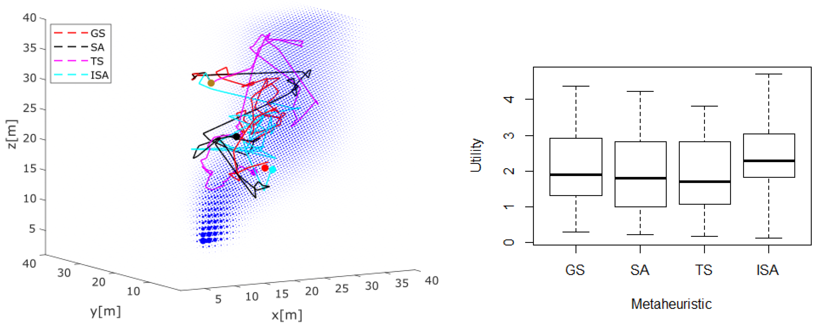
4.3. Performance Evaluation

The performance of the algorithms is evaluated with three indicators:
  • The energy consumption, which determines the efficiency of the algorithm to trace the pollutant plume, following the shortest and smoothest path;
  • The average level of the pollutant measurements during the search, which defines the quality of the algorithm for following always the direction towards the increasing pollutant concentration; and
  • The distance to the real location of the source at the end of the simulation, which indeed is the goal of the algorithms.
The following equation defines the utility to evaluate the methods:
U M = U E C + U P L + U D S
where U M is the utility of the method M; U E C , U P L and U D S are the utilities of the energy consumption, the average pollutant level and the distance to the source, respectively, given as follows:
U E C = η e c B ¯
U P L = η p l P a
U D S = η d s d s
where η e c , η p l and η d s ( η e c > η d s > η p l ) are the weight of utility for each component, B ¯ is the remaining battery of the UAV at the end of the mission, d s is the final distance of the UAV to the source and P a is the average of the pollutant captured during the mission.

4.4. Results of the Comparative Analysis

To evaluate the performance of the above algorithms, 100 simulation experiments were carried out under two conditions of the environment. First, an environment with low and constant wind was tested as shown in the example in Figure 3. Under these conditions, the algorithms reached the source most of the times. An environment with highly-variant wind effects was also tested, as shown in the example in Figure 4. In this configuration, the GS maintained its average utility, the TS increased its utility in about 12%, the SA increased its average utility in about 15% and the ISA average utility was reduced in about 20%.
According to the box-plot of the algorithm’s performance analysis, shown in Figure 3 and Figure 4, the ISA approach maintains a superior performance in the highly variant environments.
When introducing the component of velocity towards the positions with high levels of the pollutant concentration, the basic simulated annealing methodology improved significantly. This fact will be exploited in the next section for designing the final algorithm to localize the source of the pollutant.

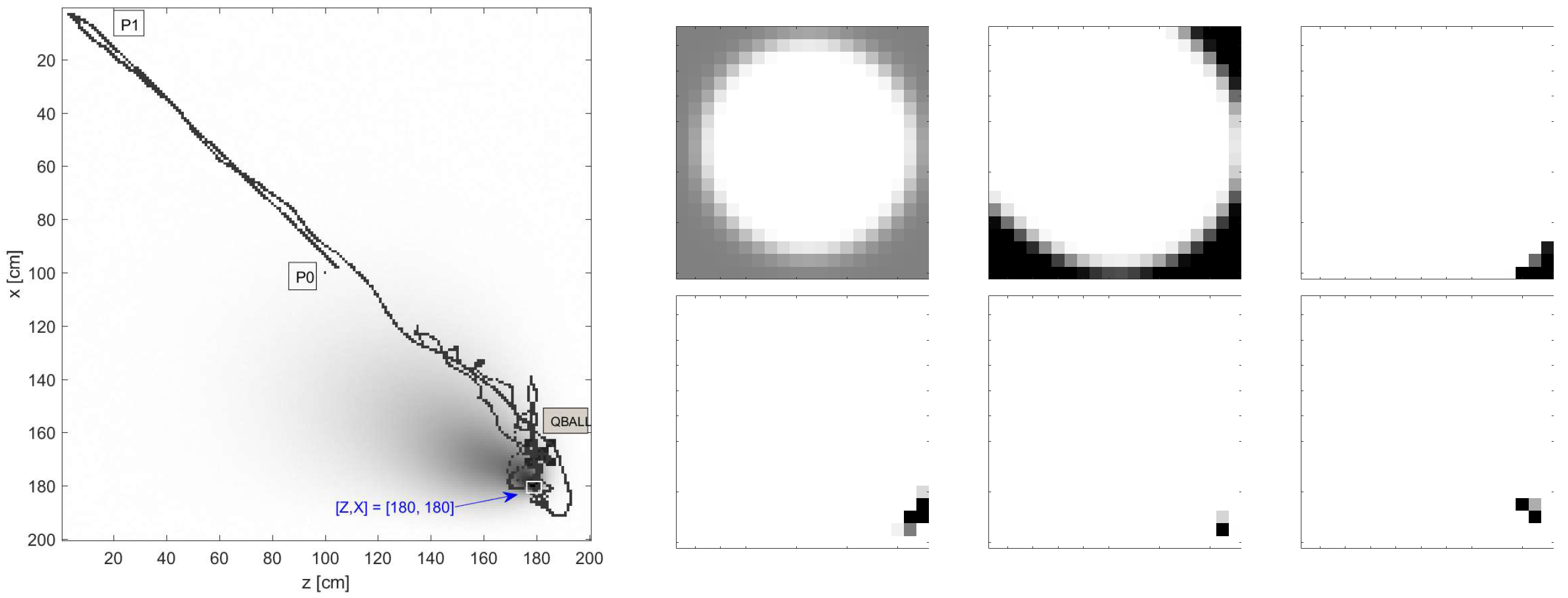
5. Pollutant Source Localization

The gradient-based metaheuristic demands that the UAV starts the navigation from inside the pollutant plume or at least close to it. Otherwise, the UAV navigates in arbitrary directions. In addition, when the UAV losses the direction with ascending gradient, a new direction is required in the tracing process. These issues can be solved by integrating with the metaheuristic algorithm, a heuristic of the source position, herein named h, calculated from a likelihood map of the location of the source (Section 5.1). This component herein is called probabilistic.
While the UAV uses the gradient-based technique (ISA) to find increasing concentration of the pollutant, the heuristic h is introduced to adjust the directions calculated by the metaheuristic algorithm to guide the search to the most promising regions of the pollutant concentrations.
To get the final design of the algorithm, joining the metaheuristic and the probabilistic approaches, the problem of the localization of the pollutant source was reduced to two dimensions. This reduction does not limit the potential of the development. Indeed, some insects like moths, limit their search to the horizontal planes [22]. Besides, the air pollution propagation effect in the vertical direction is much weaker than the horizontal direction [31], and the effects of the UAV presence in pollutant measurements [6,7,8] will be weaker if the UAV only performs two dimensional trajectories. With this simplification, the solution will require less processor capacity, that is, lower energy consumption, allowing for the search to be extended to larger areas.

5.1. Likelihood Map for Source Localization

Following the work presented in Reference [25], a Likelihood Map for the Location of the Source (LMLS) was created. This methodology assumes that the UAV can measure or estimate the pollutant concentration and the wind velocity at its current position.
The LMLS construction is based on the Bayesian methodology. In this algorithm, the first step is to create the LMLS representation, dividing in cells the targeted environment. Let us denote the X and Z axis, according to the environment shown in Figure 5. Splitting the total area of the environment in rectangular cells, with longitudes L x and L z , in the X and Z directions respectively, the m × n cellular subdivisions can be obtained. The resulting cells are defined by the vector C = [ C 1 , . . . , C M ] , where M = m × n , and the element C i represents the position ( x i , z i ) of the center of the cell i.
The goal of this step in the algorithm is to estimate a vector α i that represents the probability of the source location at cell C i ϵ C. In this work, a unique source is assumed to exist, that is, P ( α i ) = 1 .
Let A i be the event of a source being located in cell C i when the UAV, which is on cell C j , detects (event D j ( t q ) ) or not (event D ¯ j ( t q ) ) the pollutant at time t q . Note that the sensor information is binary, which is defined by using a threshold, and with this information define a vector of events, e.g., B ( t q 1 ) = { D j 1 ( t q 1 ) , D ¯ j 2 ( t q 2 ) , . . . , D j q ( t 0 ) } of detection and non-detection events from t 0 to t q 1 . Let { α ( t q 1 ) = P ( A i | B ( t q 1 ) ) } i = 1 M represent the LMLS based on detection and non-detection events B ( t q 1 ) between time t 0 and t q 1 . The aim is to update the probabilities in A using the events in B. Figure 6 summarizes how to update α i recursively, including the historical events and the Bayesian methodology.
In Figure 6, to update α i , the detection D and non-detection D ¯ events are included as follows:
P ( A i | B ( t q 1 ) , D j ( t q ) ) = M α i ( t q 1 ) β i j ( t 0 , t q )
P ( A i | B ( t q 1 ) , D ¯ j ( t q ) ) = α i ( t q 1 ) γ i j ( t 0 , t q ) M Σ i = 1 M γ i j ( t 0 , t q )
where
β i j ( t 0 , t q ) = 1 q Σ l = 0 q l S i j ( t l , t q )
γ i j ( t 0 , t q ) = Π l = 0 q 1 [ 1 μ S i j ( t l , t q ) ]
S i j ( t l , t q ) = e ( x j x i v x ( t l , t q ) ) 2 2 ( t q t l ) σ x 2 e ( z j z i v z ( t l , t q ) ) 2 2 ( t q t l ) σ z 2 2 π ( t q t l ) σ x σ z L x L z
and
V ( t l , t q ) = Σ i = l q 1 U ( P u a v ( t i ) ) d t
where U ( P u a v ( t i ) ) herein represents the wind velocity measured by the UAV at the time t i and μ is the probability of detecting pollutant in cell C j given that there is a detectable pollutant in that cell. Further explanations are presented in Reference [25], including the deductions of each equation and the optimization of the numerical processing.

5.2. Integrated Algorithm

Figure 7 shows the complete proposed algorithm, which integrates the heuristic, calculated on the base of the LMLS, to the metaheuristic algorithm. Processes in red are performed at each time t q and those filled with blue run at time t k , with t q < < t k .
In the algorithm, the first step is to get the initial heuristic ( h 0 ) of the location of the source in the environment. This is solved by using the LMLS calculated with an initial deterministic navigation of the UAV. The heuristic h ( t k ) of the source location is the position with the highest probability in the LMLS at time t k . The next steps guide the algorithm to use h obtained from LMLS, which is continuously updated according to new binary sensor information and the Bayesian methodology previously presented.
The metaheuristic process loop calculates the positions to move the UAV among the waypoints p k . To verify increasing concentration of pollutant, between the positions p k 1 and p k , the historical information captured in ψ k = { ψ ( t ) : p ( t ) ϵ ( p k 1 , p k ) } is used.
The path planning algorithm will help in the navigation of the UAV to reach each waypoint p k calculated in the metaheuristic loop. This algorithm will grant the finding of the shortest path among the waypoints but avoiding any possible obstacles in dynamic unknown terrains. In addition, the path planning algorithm will depend on partial information of the environment and the obstacle detection sensors in at least one direction, however this approach goes beyond the scope of this work, where the experiments were limited to obstacle-free environment, and the path planning calculates direct trajectories among the positions p k .
To estimate the source location, at each time t q , the historical information of concentration measurements is used. The centroid of the three positions with the highest concentration of pollutant represents the source location. If insignificant concentrations are found in the whole searching process or the procedure stops when the initial deterministic navigation has not finished, the source position is defined using the LMLS, as the cell with the higher probability.
The algorithm conditions to stop include—low battery of the UAV, very high concentration of pollutant found, maximum number of waypoints set by the user and emergency stopping. Regardless of the stopping condition and time, the proposed method will always return the most probable source location.

5.3. Inclusion of the Heuristic

According to Figure 7, the heuristic h ( t k ) influences the calculation of the next position p k + 1 , when the UAV losses the direction of the increasing pollutant concentration and λ Λ . For this condition, the current direction of the vehicle θ k is influenced by the direction to the heuristic position h ( t k ) as follows:
p k + 1 = p k + θ h ( t k ) 1 [ ψ k ] γ + β
where:
p k , p k + 1 = current and calculated positions of the vehicle;
γ = a real number that means the waypoints resolution, defined according to the UAV capacity and the environment dimension. High values of γ remains at large distances among the calculated waypoints p k . Conditions of a large targeted environment and low GPS resolution of the UAV will require high γ values;
β = a real random vector that means the deviation parameter, which allows small deviations, from the calculated waypoint p k , to compensate the stochastic behavior of the system. Low values of β are recommended;
θ h ( t k ) = a real vector that means the direction of the current position of the UAV to the most probable region of the source location, obtained from the LMLS; and
[ ψ k ] = a real number that represents the average of historical pollutant information captured from p k 1 to p k . This parameter helps to establish smaller steps of movements of the UAV in regions with high concentrations of the pollutant.
To complete the algorithm, if the UAV found a direction of increasing pollutant concentration or λ < Λ , the vehicle decides to follow this direction, and the position is calculated as follows:
p k + 1 = p k + θ k 1 [ ψ k ] γ + β
where θ k is the vector of the current direction of the UAV, and as in the previous case, the average of the measurements in [ ψ k ] avoids abandoning the areas with high concentrations of pollutant.

6. Experiments and Results

Instead of using only a pure simulation testbed, the proposed strategy was tested with a real UAV navigating in a two-dimensional simulated polluted environment. The physical UAV in the simulated environment added constraints related to autonomy, velocity and inaccurate movements of the UAV, the last one producing irregular measurements of the pollutant. In a later stage of this research, we intend to test the algorithms with UAVs flying in real polluted scenarios.
In order to measure the performance of the algorithm, the distance from the real source location to the source location position estimated by the algorithm is considered.

6.1. Experiment Design

Figure 8 presents the overall indoor experimental test environment. This system consists of a quadrotor Qball (Quanser) with a QuaRC-powered Gumstix embedded computer onboard, for the real-time control of the vehicle [32,33]. Because the lack of GPS signals indoors, a network of 24 Opti-Track cameras is adopted for providing position and orientation information to the UAV’s embedded computer and a ground station for command allocation and real-time data display.
The area available for experimentation is a 2 m × 2 m space, at a constant altitude 0.7 m. The global positioning is based on the following coordinates: X = [ 0 , 2 ] m and Z = [ 0 , 2 ] m.
The positioning of the quadrotor is controlled through the Gumstix computer on-board of the quadrotor, using data of the IMU and the Opti-track Visual system and a Kalman filter to correct the position and orientation of the UAV. The quadrotor is constrained to the maximum linear velocities of v x = 0.15 m/s and v z = 0.15 m/s. For heading the velocity is limited to ( 15 p i / 180 ) rad/s. A simulated polluted environment with high advection was used, according to the dispersion model of pollutants previously explained, including dispersion, wind effects and stochastic noises.
The cyber-sensors onboard the UAV captures the pollutant and wind vector in the physical position of the UAV. In the real application, the wind vector must be estimated, that is, the magnitude and the direction. The dynamic of a real environment have been included in the model used in the experiments, as explained in Section 2.
The fixed initial position of the quadrotor for any mission is at ( Z , X ) = ( 100 , 100 ) cm. Given the limited testing area, the numbers of waypoints were restricted to a maximum of 30 for each experiment. The vehicle starts performing a deterministic navigation to get the initial heuristic position and then the metaheuristic algorithm guides the vehicle while the LMLS is updated and used by the UAV to follow the most promising position of the source location.
The parameters selected for the LMLS of the experiments were: L x = 10 cm, L z = 10 cm, σ x 2 = 10 c m 2 s , σ z 2 = 10 c m 2 s and the probability μ = 0.95 .

6.2. Experiments

Three experiments were performed to analyze the effectiveness and robustness of the proposed algorithm. Figure 9 and Figure 10 show the results of the experiments 1 and 2, respectively. In both experiments, the UAV starts with a deterministic navigation from the point P 0 to P 1 and uses the information of the binary sensor and winds effects to construct and update the LMLS, which was initiated as uniform. In these trajectories, the binary sensor did not detect the pollutant concentrations, but the information is useful to generate the initial heuristic position of the source h 0 .
From the position P 1 , the UAV is guided by the proposed strategy combining the metaheuristic component, to trace the increasing direction of the pollutant concentration, and the probabilistic component which helps the UAV to remain in the areas with high probability to find the pollutant source.
In the experiment 1, the pollutant is released in the position ( Z , X ) = ( 180 , 180 ) cm and the algorithm calculates the source position at ( Z , X ) = ( 179.1 , 180.1 ) cm. In the experiment 2, the pollutant is released in the position ( Z , X ) = ( 20 , 180 ) cm and the algorithm determines the source position at ( Z , X ) = ( 20.29 , 180.7 ) cm.
Figure 11 shows experiment 3. In this experiment, the winds effects were increased, mimicking more complex environment. The pollutant was released in the position ( Z , X ) = ( 170 , 50 ) cm and the algorithm calculated the source position at ( Z , X ) = ( 168.2 , 45.62 ) cm.
As shown, the algorithm has high effectiveness. In addition, the parameters of the algorithm have not been changed for the different experiments, that is, the algorithm is robust.
The real UAV showed high variation in the path while the vehicle was driven among the waypoints. Despite this fact, the vehicle was able to approach very close to the source.
The source location was estimated on each time, using the information of the visited positions and the heuristic calculated from the LMLS. This is useful for applications in environments where the source position is not reachable by the UAV but could be estimated by the algorithm.
The waypoints resolution was set to 30 cm, given the environment and vehicle dimensions. This restriction complicates the searching since when the metaheuristic algorithm finds the direction of the positive gradient of pollutant, it follows this direction to calculate the new waypoint with the defined resolution and the vehicle has high probabilities of leaving the plume of pollutant. On the other hand, this minimum resolution is useful since a path planning algorithm can be used to operate the UAV in an environment with static or dynamic obstacles.
As the algorithm was based on two independent approaches, the minimum waypoints resolution was outperformed successfully. The heuristic position aided maintaining the exploration in the most promising areas while the metaheuristic facilitated the exploration the increasing gradient of pollutants in these areas.
The algorithm implementation requires the tuning of some parameters. The calculus of the LMLS includes the parameters: L x , L z , σ x , σ z and μ . To select L x and L z , a trade-off between an accurate heuristic and low computational cost should be considered. The parameters σ x and σ z allow the tuning of the convergence velocity of the likelihood probability distribution in the map. The parameter μ can be estimated by evaluating the sensor reliability in the pollutant measurement.
In addition, as explained before, the information of the sensor for the LMLS updating is binary. This information is obtained by passing the raw measurement of the sensor through a defined threshold. The threshold must be sufficiently high to evade the noise levels but without getting an insensitive binary sensor. Also, the wind vector is required to be estimated in each position but, as the method is probabilistic, a mean approximation of these effects over the environment is enough.
On the part of the metaheuristic algorithm, the parameters T 0 , Δ T and ϵ must be adequately set. The temperature parameters T 0 and Δ T are selected such that temperature T must be maintained greater than zero and also its quick decrement must be avoided. The parameter ϵ helps us to analyze whether the vehicle has found increasing pollutant gradients avoiding the noise levels. The analysis of the pollutant targeted and the sensor used would be indispensable for the gradient increasing definition.

7. Conclusions

This work presents an algorithm for pollutant source localization using a UAV, which takes advantages of the greedy-based metaheuristic to trace the pollutant plume and the Bayesian methodology to create a probabilistic map of the source location. A comparative analysis of some metaheuristic methods allowed us to define the most effective approach for tracing the pollutant plume. To complement this strategy, the probabilistic component provided a heuristic position which helped us to reduce the searching area each time to the most probable position of the source location.
Instead of using only a pure simulated experimental testbed, the algorithm was tested using a real UAV navigating in a virtual polluted environment with high turbulence. This hybrid environment adds the real constraints of the navigation of the UAV and the sensing of the pollutant. The results showed the effectiveness and robustness of the proposed algorithm. The design of the proposed strategy is general and can be adapted to localize any air pollutant source. The next step in this research is the testing of the algorithm with a physical UAV flying in a real polluted environment.

Author Contributions

Conceptualization and methodology, N.Y.-N. and L.E.G.-C.; software and validation, N.Y.-N.; formal analysis, N.Y.-N. and L.I.M.-A.; investigation, N.Y.-N. and L.E.G.-C.; resources, Y.Z.; writing—original draft preparation, N.Y.-N.; writing—review and editing, L.I.M.-A. and Y.Z.; supervision, L.E.G.-C. and Y.Z.; funding acquisition, L.E.G.-C. and Y.Z.

Funding

This research received no external funding.

Acknowledgments

The first author would like to thank to CONACYT for the grant financial aid to develop the project and to Concordia University for allowing the use of the lab facilities for performing the experimental tests.

Conflicts of Interest

The authors declare no conflict of interest.

References

  1. World Health Organization. Ambient Air Pollution: A Global Assessment of Exposure and Burden of Disease; Technical report; WHO: Geneva, Switzerland, 2016; Available online: http://www.who.int/phe/publications/air-pollution-global-assessment/en/ (accessed on 30 August 2019).
  2. Stieb, D.M.; Chen, L.; Hystad, P.; Beckerman, B.S.; Jerrett, M.; Tjepkema, M.; Crouse, D.L.; Omariba, D.W.; Peters, P.A.; van Donkelaar, A.; et al. A national study of the association between traffic-related air pollution and adverse pregnancy outcomes in Canada, 1999–2008. Environ. Res. 2016, 148, 513–526. [Google Scholar] [CrossRef] [PubMed]
  3. Carugno, M.; Consonni, D.; Randi, G.; Catelan, D.; Grisotto, L.; Bertazzi, P.A.; Biggeri, A.; Baccini, M. Air pollution exposure, cause-specific deaths and hospitalizations in a highly polluted Italian region. Environ. Res. 2016, 147, 415–424. [Google Scholar] [CrossRef] [PubMed] [Green Version]
  4. Sepúlveda, F. Air Pollution And Sick Leaves: The Child Health Link. Hitotsubashi J. Econ. 2014, 2014, 109–120. [Google Scholar]
  5. Van der Zee, S.C.; Fischer, P.H.; Hoek, G. Air pollution in perspective: Health risks of air pollution expressed in equivalent numbers of passively smoked cigarettes. Environ. Res. 2016, 148, 475–483. [Google Scholar] [CrossRef] [PubMed] [Green Version]
  6. Villa, T.F.; Salimi, F.; Morton, K.; Morawska, L.; Gonzalez, F. Development and Validation of a UAV Based System for Air Pollution Measurements. Sensors 2016, 16, 2202. [Google Scholar] [CrossRef]
  7. Zhou, X.; Aurell, J.; Mitchell, W.; Tabor, D.; Gullett, B. A small, lightweight multipollutant sensor system for ground-mobile and aerial emission sampling from open area sources. Atmos. Environ. 2017, 154, 31–41. [Google Scholar] [CrossRef] [PubMed] [Green Version]
  8. Roldán, J.J.; Joossen, G.; Sanz, D.; del Cerro, J.; Barrientos, A. Mini-UAV based sensory system for measuring environmental variables in greenhouses. Sensors 2015, 15, 3334–3350. [Google Scholar] [CrossRef]
  9. Kersnovski, T.; Gonzalez, F.; Morton, K. A UAV system for autonomous target detection and gas sensing. In Proceedings of the 2017 IEEE Aerospace Conference, Big Sky, MT, USA, 4–11 March 2017; pp. 1–12. [Google Scholar] [CrossRef]
  10. Malaver, A.; Motta, N.; Corke, P.; Gonzalez, F. Development and integration of a solar powered unmanned aerial vehicle and a wireless sensor network to monitor greenhouse gases. Sensors 2015, 15, 4072–4096. [Google Scholar] [CrossRef]
  11. Peng, C.C.; Hsu, C.Y. Integration of an unmanned vehicle and its application to real-time gas detection and monitoring. In Proceedings of the 2015 IEEE International Conference on Consumer Electronics, Taipei, Taiwan, 6–8 June 2015; pp. 320–321. [Google Scholar] [CrossRef]
  12. Villa, T.F.; Gonzalez, F.; Miljievic, B.; Ristovski, Z.D.; Morawska, L. An Overview of Small Unmanned Aerial Vehicles for Air Quality Measurements: Present Applications and Future Prospectives. Sensors 2016, 16, 1072. [Google Scholar] [CrossRef]
  13. Alvear, O.; Zema, N.R.; Natalizio, E.; Calafate, C.T. Using UAV-Based Systems to Monitor Air Pollution in Areas with Poor Accessibility. J. Adv. Transp. 2017, 2017, 14. [Google Scholar] [CrossRef]
  14. Kristiansen, R.; Oland, E.; Narayanachar, D. Operational concepts in UAV formation monitoring of industrial emissions. In Proceedings of the 2012 IEEE 3rd International Conference on Cognitive Infocommunications (CogInfoCom), Kosice, Slovakia, 2–5 December 2012; pp. 339–344. [Google Scholar] [CrossRef]
  15. Han, J.; Xu, Y.; Di, L.; Chen, Y. Low-cost multi-UAV technologies for contour mapping of nuclear radiation field. J. Intell. Robot. Syst. 2013, 2013, 1–10. [Google Scholar] [CrossRef]
  16. Shen, Z.; He, Z.; Li, S.; Wang, Q.; Shao, Z. A multi-quadcopter cooperative cyber-physical system for timely air pollution localization. ACM Trans. Embed. Comput. Syst. (TECS) 2017, 16, 70. [Google Scholar] [CrossRef]
  17. Hu, S.C.; Wang, Y.C.; Huang, C.Y.; Tseng, Y.C. Measuring air quality in city areas by vehicular wireless sensor networks. J. Syst. Softw. 2011, 84, 2005–2012. [Google Scholar] [CrossRef]
  18. Alvear, O.; Calafate, C.T.; Zema, N.R.; Natalizio, E.; Hernández-Orallo, E.; Cano, J.C.; Manzoni, P. A Discretized Approach to Air Pollution Monitoring Using UAV-based Sensing. Mob. Netw. Appl. 2018, 23, 1693–1702. [Google Scholar] [CrossRef] [Green Version]
  19. Yungaicela-Naula, N.M.; Zhang, Y.; Garza-Castañon, L.E.; Minchala, L.I. UAV-based Air Pollutant Source Localization Using Gradient and Probabilistic Methods. In Proceedings of the 2018 International Conference on Unmanned Aircraft Systems (ICUAS), Dallas, TX, USA, 12–15 June 2018; pp. 702–707. [Google Scholar]
  20. Cabrita, G.; de Sousa, P.A.M.; Marques, L. Odor Guided Exploration and Plume Tracking-Particle Plume Explorer. 2011, pp. 183–188. Available online: https://pdfs.semanticscholar.org/bf01/5fc709514c0dc3658c3d3b804feb20c44b62.pdf (accessed on 30 August 2019).
  21. Passino, K.M. Biomimicry of bacterial foraging for distributed optimization and control. IEEE Control Syst. 2002, 22, 52–67. [Google Scholar]
  22. Marques, L.; Nunes, U.; de Almeida, A.T. Olfaction-based mobile robot navigation. Thin Solid Film. 2002, 418, 51–58. [Google Scholar] [CrossRef] [Green Version]
  23. Nurzaman, S.G.; Matsumoto, Y.; Nakamura, Y.; Koizumi, S.; Ishiguro, H. Biologically inspired adaptive mobile robot search with and without gradient sensing. In Proceedings of the 2009 IEEE/RSJ International Conference on Intelligent Robots and Systems, St. Louis, MO, USA, 10–15 October 2009; pp. 142–147. [Google Scholar] [CrossRef]
  24. Neumann, P.P.; Hernandez Bennetts, V.; Lilienthal, A.J.; Bartholmai, M.; Schiller, J.H. Gas source localization with a micro-drone using bio-inspired and particle filter-based algorithms. Adv. Robot. 2013, 27, 725–738. [Google Scholar] [CrossRef]
  25. Pang, S.; Farrell, J.A. Chemical plume source localization. IEEE Trans. Syst. Man Cybern. Part B (Cybernetics) 2006, 36, 1068–1080. [Google Scholar] [CrossRef]
  26. Van Milligen, B.P.; Bons, P.D.; Carreras, B.A.; Sánchez, R. On the applicability of Fick’s law to diffusion in inhomogeneous systems. Eur. J. Phys. 2005, 26, 913. [Google Scholar] [CrossRef]
  27. Hosseinin, B. Dispersion of Pollutants in the Atmosphere: A Numerical Study. Master’s Thesis, Simon Fraser University, Burnaby, BC, Canada, 2013. [Google Scholar]
  28. Šmídl, V.; Hofman, R. Tracking of atmospheric release of pollution using unmanned aerial vehicles. Atmos. Environ. 2013, 67, 425–436. [Google Scholar] [CrossRef]
  29. Gendreau, M.; Potvin, J.Y. Handbook of Metaheuristics; Springer: Berlin, Germany, 2010; Volume 2. [Google Scholar]
  30. Aarts, E.; Korst, J.; Michiels, W. Simulated annealing. In Search Methodologies; Springer: Berlin, Germany, 2014; pp. 265–285. [Google Scholar]
  31. Daly, A.; Zannetti, P. Air Pollution Modeling—An Overview. Available online: http://envirocomp.org/books/chapters/2aap.pdf (accessed on 12 April 2018).
  32. Liu, Z.; Yuan, C.; Yu, X.; Zhang, Y. Retrofit fault-tolerant tracking control design of an unmanned quadrotor helicopter considering actuator dynamics. Int. J. Robust Nonlinear Control 2017. [Google Scholar] [CrossRef]
  33. Wang, B.; Zhang, Y. An Adaptive Fault-Tolerant Sliding Mode Control Allocation Scheme for Multirotor Helicopter Subject to Simultaneous Actuator Faults. IEEE Trans. Ind. Electr. 2017, 65, 4227–4236. [Google Scholar] [CrossRef]
Figure 1. Simulated annealing algorithm.
Applsci 09 03712 g001
Figure 2. Parametrization of the Simulated Annealing (SA) methodology.
Applsci 09 03712 g002
Figure 3. Example of simulation using different metaheuristics for plume tracing in environments with constant winds.
Applsci 09 03712 g003
Figure 4. Example of simulation using different metaheuristics for plume tracing in environments with highly-variant wind effects.
Applsci 09 03712 g004
Figure 5. Cells representation of the splitted targeted area.
Applsci 09 03712 g005
Figure 6. Updating methodology of the LMLS.
Applsci 09 03712 g006
Figure 7. Pollutant source localization algorithm.
Applsci 09 03712 g007
Figure 8. Indoor experimental test environment.
Applsci 09 03712 g008
Figure 9. Experiment 1. Mission for the pollutant source localization. At the left is the source localization mission using the Qball. At the right are the LMLS updated at the times [105.4, 112.6, 122.3, 122.9, 126.1, 139.3] seconds (left to right and top to bottom).
Applsci 09 03712 g009
Figure 10. Experiment 2. Mission for the pollutant source localization with different source position. At the left is the source localization mission using the Qball. At the right are the Likelihood Map for the Location of the Source (LMLS) updated at the times [104.9, 111.1, 121.7, 126.7, 126.4, 142.3] seconds (left to right and top to bottom).
Applsci 09 03712 g010
Figure 11. Experiment 3. Mission for the pollutant source localization with high wind effects. At the left are the LMLS updated at the times [123.44, 127.04, 136.64, 137.44, 146.04, 158.44] seconds (left to right and top to bottom).
Applsci 09 03712 g011

