Article

An End-to-End Deep Learning Image Compression Framework Based on Semantic Analysis

School of Electronic Engineering, Beijing University of Posts and Telecommunications, Beijing 100876, China
*
Author to whom correspondence should be addressed.
Appl. Sci. 2019, 9(17), 3580; https://doi.org/10.3390/app9173580
Submission received: 26 July 2019 / Revised: 22 August 2019 / Accepted: 23 August 2019 / Published: 1 September 2019

Abstract

:
Lossy image compression can reduce the bandwidth required for image transmission in a network and the storage space of a device, which is of great value in improving network efficiency. With the rapid development of deep learning theory, neural networks have achieved great success in image processing. In this paper, inspired by the diverse extent of attention in human eyes to each region of the image, we propose an image compression framework based on semantic analysis, which creatively combines the application of deep learning in the field of image classification and image compression. We first use a convolutional neural network (CNN) to semantically analyze the image, obtain the semantic importance map, and propose a compression bit allocation algorithm to allow the recurrent neural network (RNN)-based compression network to hierarchically compress the image according to the semantic importance map. Experimental results validate that the proposed compression framework has better visual quality compared with other methods at the same compression ratio.

1. Introduction

The rapid development of the Internet of Things (IoT) has greatly facilitated people’s lives, and it has also led to an explosive increase in the amount of data transmitted by networks. The types of network services have developed from the original text and voice signals to image and video signals, which brings convenience for the transmission of information and also continuously improves the requirements for data transmission and storage. Therefore, in order to reduce the volume of images during transmission and storage to improve network transmission efficiency, obtaining a better recovery quality through a smaller compression size has long been the focus of research in the image field.
Image compression technology can be generally divided into lossy compression and lossless compression. Lossless compression compresses images by removing statistical redundancy in the image [1]. The process is reversible and is usually used in scenes where image sharpness is high, such as medical images, such as performed in [2], scarce data images and so on. The lossy compression algorithm performs redundant processing on image information according to the principle that the human eye is insensitive to certain visual features. Compared with lossless compression technology, lossy compression is at the expense of removing invisible information from the human eye, in exchange for the promotion of the compression ratio. Common lossy compression algorithms can be divided into traditional methods based on mathematical statistics and neural network methods based on deep learning. Most of the traditional methods are considered from the statistical characteristics of the data and compress images by various mathematical algorithms; typically, these include predictive coding, as used in [3]; sub-band coding, as in [4]; JPEG, as in [5], and so on. Deep learning-based methods mostly use artificial neural networks to design image codecs. Benefitting from the strong learning ability of the neural network, these methods can study the characteristics of images through backpropagation and realize the compression of image information without too much prior knowledge.
Although many methods of deep learning currently perform well in image compression, there are still several issues to be addressed. In general, the human eye has a different degree of attention to each area of the image. For example, in a portrait picture, the clarity and texture details of the characters in the foreground are more eye-catching than the background. With the current IoT multimedia data compression requirements, most images have an apparent distinction between the foreground and background. However, the existing compression method performs the same processing for each pixel of the picture, so in an image with low background importance, it does not make the best allocation for each compressed bit. Therefore, in this scenario, it is necessary to propose the corresponding compression technique for the optimal compression bit allocation problem with clear foreground–background discrimination images. At present, most of the pictures on the Internet will generate noise during the transmission process, which will have a negative impact on the compression and recovery of the images. Some excellent denoising methods have been proposed in [6], [7] and [8]. In the experiments in this paper, we used the Kodak dataset without noise to better verify the performance of the compression algorithm.
The proposed image compression framework in this paper is shown in Figure 1, including the semantic analysis network and image compression network. We use the semantic analysis network to extract the essential semantic regions of the input image and calculate the compression level corresponding to each area and then use the image compression network to compress and decompress the image hierarchically.
The specific contributions are divided into the following three points:
(1) An end-to-end deep learning image compression framework based on semantic analysis is proposed, containing a semantic analysis network based on a convolutional neural network (CNN) and an image compression network based on a recurrent neural network (RNN).
(2) We design a compression bit allocation algorithm to calculate the compression iterations of each image block, skillfully using the results of semantic analysis to compress the image hierarchically.
(3) The performance and feasibility of the proposed compression framework are verified by comparison with other image compression algorithms in a multi-structure structural similarity (MS-SSIM) index and proposed semantic–important structural similarity (SI-SSIM) index.

2. Related Works

Recently, benefitting from the generation of large-scale data sets, the development of robust models, and a large number of available computing resources, deep learning theory has made excellent progress in the field of image semantic analysis and image compression. The weakly supervised semantic classification network is booming with the rise of deep learning, allowing computers to understand pictures better. As the originator of the CNN network, LeNet [9] is composed of a convolution layer, pooling layer, full connection layer, and sigmoid as the activation function. For the first time, the convolution layer is used instead of a manual hand-craft feature, which allows the computer to understand the picture in its own way. The Imagenet Large-Scale Visual Recognition (ILSVRC) competition has stimulated the rapid development of semantic analysis networks. In 2012, AlexNet—proposed by Hinton and Alex Krizhevsky in [10]—exploited Rectified Linear Units (ReLu) as an activation function replacing sigmoid to solve gradient diffusion and adopted dropout to avoid overfitting, aiming to focus on the wider meaning of semantic feature representation. In the same year, Google Inception Net (GoogleNet) in [11] was proposed as the winner of ILSVRC. GoogleNet used a 22-layer deep network to avoid gradient disappearance, subtly adding two loss functions at different depths network to ensure the return of the gradient. In addition, a 1×1 convolution kernel was adopted to reduce the thickness of the feature map. Residual Network (ResNet), proposed by Kaiming He et al. in [12], achieved a colossal breakthrough: the bottleneck residual block and jump connection deepened the depth of the network without gradient disappearance and network degradation. The 152-layer-deep network made a great leap forward in improving the deeper semantic understanding of the image.
Deep learning has also made excellent progress in the field of image compression. A super-resolution convolutional neural network (SRCNN) network for image compression was proposed in [13] by Chao Dong et.al., first applying deep learning methods in solving pixel-level image problems. It uses a three-layer convolution structure to sample a low-resolution image by doubling the cubic difference and reconstructs the image in the pixel domain through the network. Researchers at Google proposed recurrent neural networks based on convolution and deconvolution long short-term memory (LSTM) in [14]. Four compression models were designed without retraining when the compression ratio changed, which were a full connection or convolution/deconvolution residual encoder with and without LSTM, finally using the SSIM index as the evaluation standard. Further, they published a progressive method in 2016 [15], a full-resolution image compression method based on a neural network, which achieved a 4.3–8.8% higher area under the rate-distortion curve (AUC) compared with the existing compression methods, making it the first neural network image compression framework beyond JPEG. In 2017, Mu Li et al. at Hong Kong Polytechnic University proposed an image compression method based on image content weighting in [16]. This method adds the concept of an importance map to the traditional self-encoder structure. The edge feature map extracted by the three-layer convolution neural network from the features map was output by the encoder as the importance map of the original image. However, this method focuses on the edge of objects instead of the whole region, and a certain compression ratio is maintained for each training of the network. In 2017, a CNN-based image compression framework was proposed [17] which included two CNN networks, compact convolutional neural network (ComCNN) and reconstruction convolutional neural network (RecCNN), which are used to encode and decode the original image, respectively. An innovative algorithm collaborates two CNN networks, which solves the non-differentiated calculation in the quantization rounding function to achieve a backward propagation gradient in the standard image algorithm. In 2018, an image compression scheme incorporating semantics was proposed in [18]; the authors combined image compression and classification to reconstruct the images and generate corresponding semantic representations at the same time. In 2019, Ma Siwei et al. summarized and analyzed image and video compression techniques based on deep learning [19]. In terms of image compression, the authors introduced image compression methods based on the random neural network, convolutional neural network, recurrent neural network, and generative adversarial network methods from the perspective of principle and performance.

3. Network Structure

3.1. Semantic Analysis Network

To enable the differentiated compression of the image, it is necessary to perform semantic analysis on the input image to identify an area of interest to the human eye and then allocate it more compressed bits. Although the existing techniques are able to accurately outline the boundary of the objects in the picture, this segmentation of the hard boundary of the object is not important for semantic compression, and it is critical to locate the approximate range of the object. In this paper, we use deep learning methods for image classification to achieve the annotation of semantic areas. The class activation mapping (CAM) method is proposed by Zhou in [20] to describe the possibility that each pixel belongs to a specific category. Based on the CAM method, the probability that each pixel belongs to a specific class can be converted into the semantic importance of the pixel. The higher the possibility, the higher the importance of the pixel for the picture content, and the more compression bits need to be allocated.
The semantic analysis network structure used in this paper is shown in Figure 2, using a classification-based training network architecture similar to Visual Geometry Group 16 (VGG16). The first five convolutional layers are used to extract the characteristics of the input image, and a global average pooling (GAP) layer is placed after the last convolution layer instead of the fully connected layer (FC) to convert the feature map into a feature vector. Compared to FC, GAP reduces a large number of network parameters, preventing over-fitting, and most importantly, GAP can save spatial information of images, which is significant to generate the semantic map. Finally, the weighted linear sum of the feature vector and its corresponding weight are input to the softmax layer to obtain the class activation map.
Given an input image I and a set C of categories to be identified, we can extract feature maps f u by utilizing the CNN network, which obtains the same number as categories in set C . f u is the feature map of I for the convolutional unit u after the last convolutional layer C o n v 5 , and each f u has the ability to extract features of a certain category in I . Each f u will be averaged in GAP, and multiplied by the weight α u c —the weight of convolution unit u corresponding to the class c —to obtain the possibility P c of f u belonging to c .
P c = u α u c G ( f u )
where G ( f u ) is the GAP operation of f u . We use Pc as the input to softmax layer; then, the final classification result R c can be calculated by Formula (2).
R c = exp ( P c ) c exp ( P c ) = exp ( u α u c G ( f u ) ) c exp ( u α u c G ( f u ) )
The class c with the highest probability is chosen as the classification result of the image I , and the cross-entropy of the result and the label corresponding to I are used as the loss function to train the network. Finally, we can obtain the trained weight α u c .
To visualize the effect of the network on image I , for the specific class c , we use the linear weighted sum H c of α u c and f u to represent the probability that each pixel in the image belongs to class c .
H c = u α u c f u
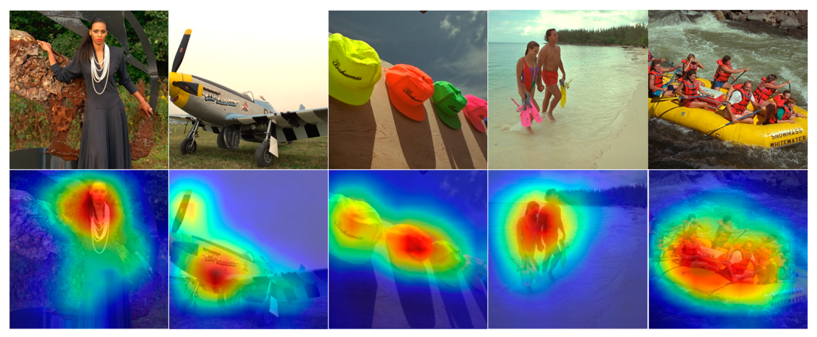
By up-sampling H c to the size of picture I and superimposing it with I , we can get the thermal maps shown in Figure 3 as the result of semantic analysis. The degree of highlighting indicates the level of semantic importance.

3.2. Image Compression Network

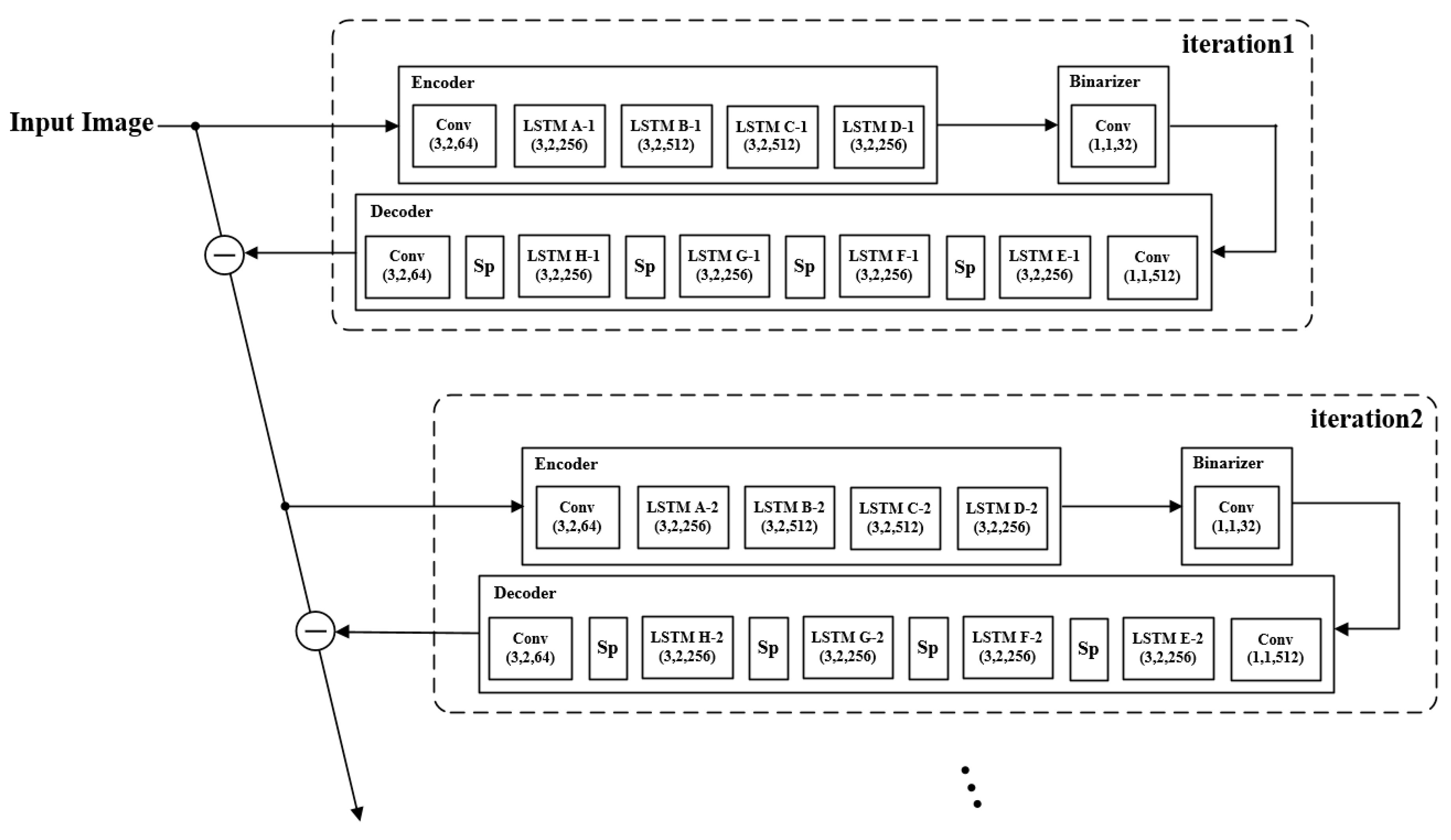
The image compression part of this paper adopts the network structure in [15]: a recurrent neural network including an encoder, binarizer, and decoder, which can be end-to-end trained. The system can perform multiple iterations, and in each iteration, the encoder E encodes the input image to a representation code; then, the binarizer B transforms the representation code into a binary code. Finally, the decoder D predicts the output image by the binary code. The residual of the output and input for each iteration will be used as the input for the next iteration. Each iteration is described as follows:
b k = B ( E k ( r k 1 ) ) , x ^ k = D k ( b k ) , r k = x x ^ k
where E k and D k , respectively, represent the encoder and decoder for the k th iteration. B denotes the binarizer, b k is the binary code in the k th iteration, x k is the predicted output of the k th iteration, and r k is the residual of the production and input for the k th iteration. The compression network consists of multiple iteration units, which are shown in Figure 4.
Each iteration unit contains convolutional units, LSTM units and a sub-pixel structure, which are used to extract image features, memorize the residuals in the iterative process, and restore the size of the image, respectively. The entire compression network uses eight recurrent neural networks composed of LSTM units (from A to H), which use the predicted output of the previous LSTM unit as inputs in a single iteration and transmit the hidden layer state parameter to the corresponding LSTM unit in the next iteration. The structure of the LSTM unit is shown in Figure 5, where c k 1 and h k 1 are the memory state and hidden layer state of the LSTM unit in the previous iteration, and x k is the input vector of the k th iteration, which is equal to the output of the upper layer network in this iteration. Each unit contains two convolutional neural networks; c o n v _ i n works on the input vector x k , and c o n v _ h i works on the hidden layer state h k 1 of the LSTM unit in the previous iteration.
For a given input vector x k , c k 1 , and h k 1 , the calculation methods of c k and h k in this iteration are as follows:
[ f , i , C ˜ , o ] T = [ σ , σ , tanh , σ ] T ( c o n v _ i n ( x k ) + c o n v _ h i ( h k 1 ) )
c k = f c k 1 + i C ˜
h k = o tanh ( c k )
where denotes element-wise multiplication.
The binarizer first uses a convolutional neural network plus a tanh activation function to map the representation code obtained by the encoder to the interval of (–1, 1), and then uses the sign function to binarize the code in the range into a set {–1, 1}. An H × W × 3 input vector can be compressed into an ( H / 16 ) × ( W / 16 ) × 32 binary code, meaning that we can obtain the bits per pixel (bpp) in each iteration as 1/8, and the compression ratio in the k th iteration is k/192.
In addition to the CNN and LSTM units, the sub-pixel structure proposed in [21] is used in the decoder to up-sample the feature vector and revert to the scale of the input image. During training, a L 1 loss is calculated on the residuals generated at each iteration:
L 1 = k = 1 K | r k | = k = 1 K | x D k ( B ( E k ( r k 1 ) ) ) |

3.3. Compressed Image with Semantic Map
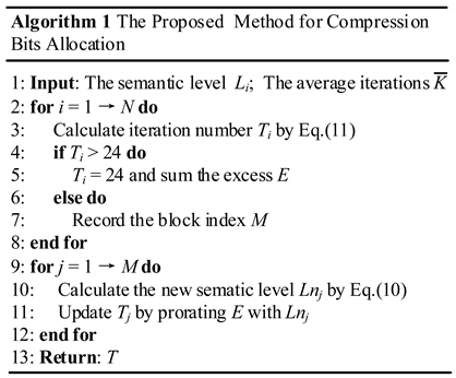
In order to perform discriminative compression for images, image blocked processing adopts 8 × 8 blocks, referring to JPEG, so that the corresponding compression ratio of each image block can be calculated according to its semantic importance, due to the problem that larger blocks will slow down the computation speed and smaller blocks will affect the information entropy between pixels. The method described in Section 3.2 is used so that the number of iterations in the image compression network controls the compression ratio of images. In this section, we propose a compression bit allocation algorithm according to the semantic importance of image blocks to calculate the number of iterations of each block given the average compression level of images.
Given the input image size H × W , the entire picture is divided into N blocks with a size of 8 × 8 , with N = H × W / 8 × 8 . Let K ¯ be the average compression level of the image, and the compression level of block i be K i ; to ensure the consistency of the compression ratio, the sum of the compression levels of all image blocks should be defined as
i = 1 N K i = K ¯ × N
We convert the semantic importance map to a grayscale graph to better represent the semantic importance of each pixel. The higher the gray value of pixel ( x , y ) , the greater the probability that i belongs to a specific grammatical category of interest to the human eye; that is, the higher the semantic importance. Let the semantic importance value V i of the block i be the sum of the gray values g ( x , y ) corresponding to each pixel ( x , y ) which belongs to the block; then, we can get the semantic level L i .
L i = V i i = 1 N V i = ( x , y ) i g ( x , y ) i = 1 N ( x , y ) i g ( x , y )
Considering the sum of the compression level of the blocks to be K ¯ × N , the calculated level of block i can be expressed as T i .
T i = L i × K ¯ × N
where · is the int function used to ensure the average compression level does not exceed K ¯ .
However, in our experiment, we found that the calculation method proposed above will result in an excessive number of iterations of the image block with higher semantic importance when the whole picture has a high average number of iterations. According to the image compression network described above, although the increase in the number of iterations can improve the quality of the restored image, a great deal of calculation time and space are required. Therefore, the allocation method is not reasonable when the average number of iterations is high, which needs further improvement.
We performed 0–30 iterative compressions on the 24 images in the Kodak dataset and calculated the corresponding MS-SSIM [22] values to verify the impact of the number of iterations on the quality of the recovered images. From the experimental results, although the recovered quality gradually improved with the increasing iterations, we observed that the degree of the improvement gradually decreased and tended to be approximate after 24 times. Therefore, we choose 24 to be the threshold for the iterations of the compression network to balance the computational overhead with the quality of the compressed image. For image blocks with more than 24 iterations, the excess number is assigned to the remaining image blocks that do not exceed this, based on the degree of semantic importance. In light of all derivations above, the complete description of the proposed algorithm is given in Algorithm 1. First, we calculated the iterations T i of each image block according to Equation (11), in which more than 24 iterations are processed as 24, and the excess part is added to the summation E . Then, we calculated the semantic level L n j of the image block not exceeding 24 times using the method in Equation (10), and finally updated T i by prorating E to these image blocks with L n j .
Applsci 09 03580 i001

4. Experiments

4.1. Traning Set

(1) Semantic analysis network
The purpose of the semantic analysis network is to identify objects that are of interest to the human eye. There are no specific requirements for the type of object. For example, it is only necessary to distinguish whether this is a dog, and it does not need to be precise whether it is a German Shepherd or a Siberian sleigh dog. Therefore, to ensure the quality of training and reduce the time of convergence, we use the Caltech-256 data set [23] to train our network—a data set specifically for image object recognition—including 256 image categories and a total of 30,608 images. We initialize the weights of the semantic analysis network using the method in [24] and using the Adam algorithm used in [25]. The learning rate is decayed from 0.01 to 0.0002 for 100 epochs.
(2) Image compression network
To reduce the training time of the compression network, we use the Cifar-100 data set [26] for training, which contains 20 significant classes, 100 subclasses, and each subclass contains 600 32 × 32 images. We initialize the weights of the image compression network using the method in [24] and the Adam algorithm used in [25]. The learning rate is decayed from 0.01 to 0.0005 for 100 epochs.

4.2. Visual Quality Evaluation

To verify the performance of the proposed compression model, we used the Kodak dataset [27] as a test to compare the results with the JPEG, BPG, and George’s methods. To fairly compare the original uncompressed images with the compressed images, it is necessary to select an evaluation indicator with a specific reference value. The fundamental purpose of the compression model proposed in this paper is to improve the subjective visual quality of human eyes. Therefore, the image will be verified using the MS-SSIM indicator, which is excellent at evaluating visual quality, applying MS-SSIM to each of the RGB channels independently to average the results. MS-SSIM gives a score of 0–1 for the contrasted picture; the closer the value to 1, the higher the similarity between the restored image and the original image.
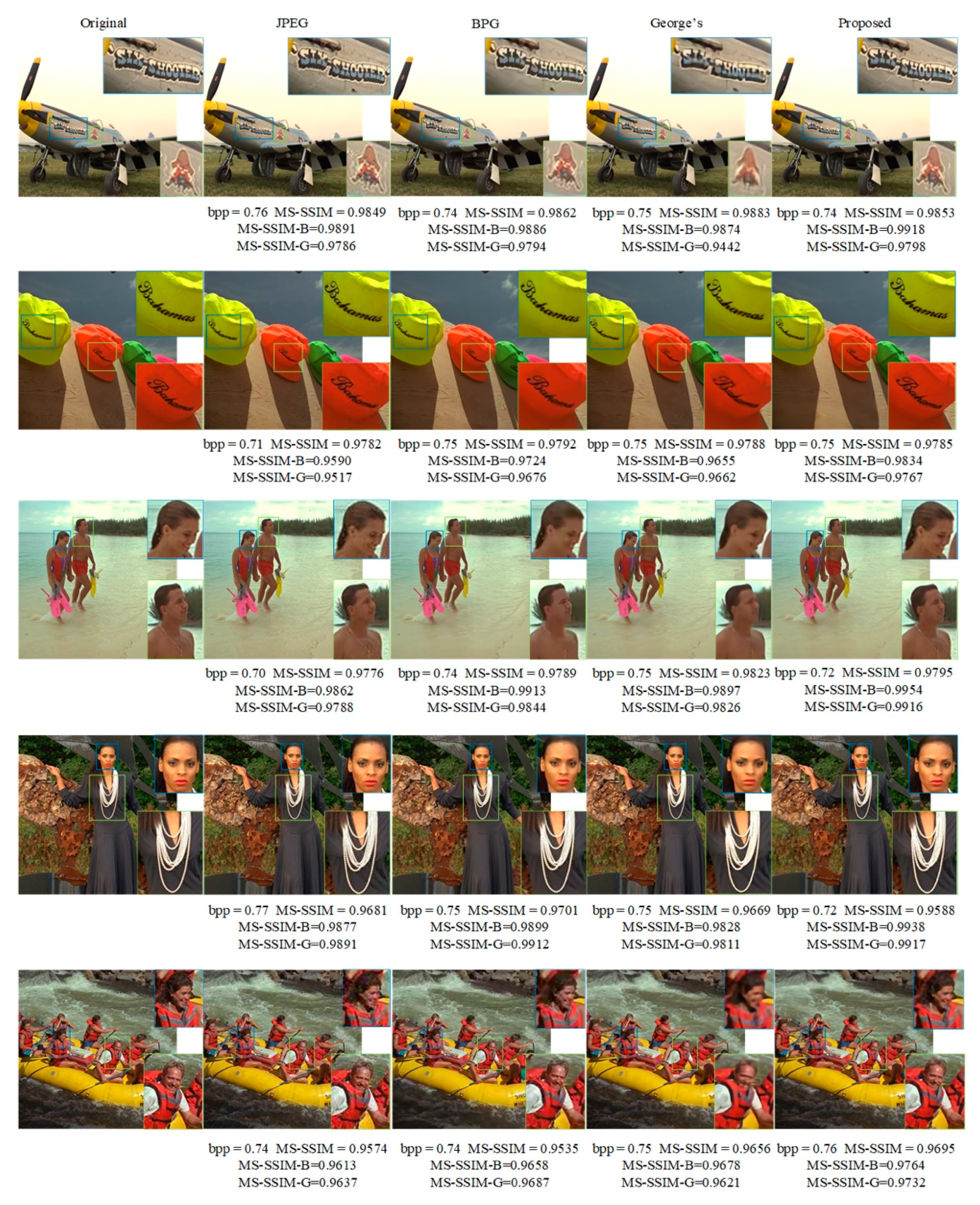
Figure 6 shows the original images and the results produced by the following compression methods. To ensure the compression ratio of each technique is as equal as possible, we maintain the bpp of the three compression methods at around 0.75; for an input RGB three-channel image, the compression ratio is close to 3 × (8/0.75) = 32 times. In the MS-SSIM indicator of the whole picture, the column of George’s method performed best, the method proposed in this paper performed less well, and the JPEG performed worst. At the same time, besides the structural similarity comparison of the whole picture, we also carried out subjective visual and objective numerical comparisons of the essential semantic areas in each image. As shown in Figure 6, the blue and green boxes are used to mark the characters and graphics on the plane, the text on the hat, the face, and the accessories on the body. All the grades of comparison in the MS-SSIM indicators show that our method gets the highest score. Moreover, in terms of visual quality, compared with the JPEG, with a visible blocking effect and artifacts through the contrast after magnification, and George’s method, with a noticeable blur in the details, our approach not only performs well in terms of sharpness and texture details but also avoids the blocking effect and artifacts that are common to JPEG methods.
The compression bit is unevenly distributed in the entire picture in our method; the higher the semantic importance, the more compressed bits are allocated in the region. In other words, compared with the average distribution compression methods, the visual recovery quality of our approach is higher than the average value in the essential semantic part and lower in the semantic inconsequential region. Therefore, the core of the compression method proposed in this paper improves the quality of essential areas by sacrificing the quality of restoration of insignificant regions to obtain better subjective visual quality. Generally speaking, the scale of the essential semantic region is usually smaller than the unimportant part of an image, which is the reason why the method in this paper is slightly inferior to George’s method in the MS-SSIM index of the whole picture.
Moreover, we compared the recovery quality of the three methods at different compression ratios. The results are shown in Figure 7a. In the case of a large compression ratio, both George’s and the improved method in this paper can obtain better performance indicators than JPEGA. However, because the method in this paper sacrifices the clarity of the background region to obtain the clarity of the essential semantic area, the MS-SSIM is slightly lower than for George’s method. Besides, we propose an SSIM evaluation index SI-SSIM based on semantic importance to distinctly reveal the improvement of the proposed method. Based on SSIM calculation, the structural similarity in semantic degree is obtained by assigning each pixel a weight corresponding to its semantic importance. The calculation of SSIM is shown in Formula (12):
S S I M ( x , y ) = ( 2 μ x μ y + c 1 ) ( 2 σ x y + c 2 ) ( μ x 2 + μ y 2 + c 1 ) ( σ x 2 + σ y 2 + c 2 )
where μ x is the average value of x , μ y is the average value of y , σ x 2 is the variance of x , σ y 2 is the variance of y , σ x y is the covariance of x and y , and c 1 and c 2 are two variables used to maintain stability. SSIM analyzes the similarity of each pixel in the two compared images, and we average the sum to get the result. In our proposed SI-SSIM, we use L i in Formula (10) as the weight of each pixel’s similarity and finally obtain the similarity based on semantic importance by averaging the weighted summation, which is shown in Formula (13). The reliability of SI-SSIM is guaranteed by verifying the Spearman rank-order correlation coefficient (SROCC), Kendall rank-order correlation coefficient (KROCC), Pearson product-moment correlation coefficient (PLCC) and root mean square error (rMSE) of SI-SSIM and SSIM.
SI-SSIM ( x , y ) = i = 1 N L i × ( ( x , y ) i S S I M ( x , y ) )
Similarly, we compared the SI-SSIM index of JPEG, BPG, George’s, and the proposed method on the Kodak dataset. The results are shown in Figure 7b, in which it can be found that the proposed methods are superior to the other two methods.

5. Conclusions

In this paper, we combine the application of deep learning in the field of image semantic analysis and image compression and propose a compression framework based on semantic analysis, consisting of a semantic analysis network and image compression network. The semantic analysis network is responsible for extracting the important semantic regions of the image using CNN and calculating the compression level according to the semantic importance of each image block. Moreover, the image compression network performs a differentiated, hierarchical compression of the image based on the calculated compression level. The experimental results demonstrate that the proposed compression method can improve the visual quality of the human eye’s attention area under the same compression overhead and has good application value in IoT image processing.

Author Contributions

C.W. was responsible for proposing the end-to-end deep learning image compression framework based on semantic analysis and designing the compression bit allocation algorithm. Y.H. performed the numerical simulations and wrote the paper. W.W. gave some suggestions on the mathematical model and formula derivation.

Funding

This work was supported by the National Key R&D Program of China (2017YFC0804400, 2017YFC0804405), the National Natural Science Foundation of China (NSFC) under Grant No. 61801033 and the Fundamental Research Funds for the Central Universities (2019RC05).

Conflicts of Interest

The authors declare no conflict of interest.

References

  1. Venugopal, D.; Mohan, S.; Raja, S. An efficient block based lossless compression of medical images. Optik 2016, 127, 754–758. [Google Scholar] [CrossRef]
  2. Ferroukhi, M.; Ouahabi, A.; Attari, M.; Habchi, Y.; Taleb-Ahmed, A. Medical Video Coding Based on 2nd-Generation Wavelets: Performance Evaluation. Electronics 2019, 8, 88. [Google Scholar] [CrossRef]
  3. Murakami, T.; Suzuki, Y. Image Decoding Device and Method Thereof Using Inter-Coded Predictive Encoding Code. U.S. Patent No. 9,414,083, 9 August 2016. [Google Scholar]
  4. Woods, J.W.; O’Neil, S.D. Sub-band coding of images. IEEE Trans. Acoust. Speech Signal Process. 1986, 34, 1278–1288. [Google Scholar] [CrossRef]
  5. Guo, L.J.; Ni, J.Q.; Shi, Y.Q. Uniform embedding for efficient JPEG steganography. IEEE Trans. Inf. Forensics Secur. 2014, 9, 814–825. [Google Scholar] [CrossRef]
  6. Sikora, T. The MPEG-4 video standard verification model. IEEE Trans. Circuits Syst. Video Technol. 1997, 7, 19–31. [Google Scholar] [CrossRef] [Green Version]
  7. Ahmed, S.S.; Messali, Z.; Ouahabi, A.; Trepout, S.; Messaoudi, C.; Marco, S. Nonparametric Denoising Methods Based on Contourlet Transform with Sharp Frequency Localization: Application to Low Exposure Time Electron Microscopy Images. Entropy 2015, 17, 3461–3478. [Google Scholar] [CrossRef] [Green Version]
  8. Ouahabi, A. A review of wavelet denoising in medical imaging. In Proceedings of the International Workshop on Systems, Signal Processing and their Applications (IEEE/WoSSPA) (2013), Algiers, Algeria, 12–15 May 2013; pp. 19–26. [Google Scholar] [CrossRef]
  9. LeCun, Y.; Bottou, L.; Bengio, Y.; Haffner, P. Gradient-based learning applied to document recognition. Proc. IEEE 1998, 86, 2278–2324. [Google Scholar] [CrossRef] [Green Version]
  10. Krizhevsky, A.; Sutskever, I.; Hinton, G.E. Imagenet classification with deep convolutional neural networks. In Proceedings of the 26th Advances in neural information processing systems, Lake Tahoe, NV, USA, 5–10 December 2013; pp. 1097–1105. [Google Scholar]
  11. Simonyan, K.; Zisserman, A. Very Deep Convolutional Networks for Large-Scale Image Recognition. arXiv 2014, arXiv:1409.1556. [Google Scholar]
  12. He, K.M.; Zhang, X.Y.; Ren, S.Q.; Sun, J. Deep residual learning for image recognition. In Proceedings of the 2016 IEEE Conference on Computer Vision and Pattern Recognition (CVPR), Las Vegas, NV, USA, 26 June–1 July 2016; pp. 770–778. [Google Scholar]
  13. Dong, C.; Loy, C.C.; He, K.; Tang, X. Learning a deep convolutional network for image super-resolution. In Proceedings of the 2014 European Conference on Computer Vision (EVVC), Zurich, Switzerland, 6–12 September 2014; pp. 184–199. [Google Scholar]
  14. Toderici, G.; O’Malley, S.M.; Hwang, S.J.; Vincent, D.; Minnen, D.; Baluja, S.; Covell, M.; Sukthankar, R. Variable Rate Image Compression with Recurrent Neural Networks. arXiv 2015, arXiv:1511.06085. [Google Scholar]
  15. Toderici, G.; Vincent, D.; Johnston, N.; Hwang, S.J.; Minnen, D.; Shor, J.; Covell, M. Full resolution image compression with recurrent neural networks. In Proceedings of the 2017 IEEE Conference on Computer Vision and Pattern Recognition, Honolulu, HI, USA, 21–26 July 2017; pp. 5435–5443. [Google Scholar]
  16. Li, M.; Zuo, W.M.; Gu, S.H.; Zhao, D.B.; Zhang, D. Learning convolutional networks for content-weighted image compression. In Proceedings of the 2018 IEEE/CVF Conference on Computer Vision and Pattern Recognition, Salt Lake City, UT, USA, 18–22 June 2018; pp. 3214–3223. [Google Scholar]
  17. Jiang, F.; Tao, W.; Liu, S.H.; Ren, J.; Guo, X.; Zhao, D.B. An end-to-end compression framework based on convolutional neural networks. IEEE Trans. Circuits Syst. Video Technol. 2018, 28, 3007–3018. [Google Scholar] [CrossRef]
  18. Luo, S.H.; Yang, Y.Z.; Song, M.L. DeepSIC: Deep Semantic Image Compression. In Proceedings of the International Conference on Neural Information Processing (ICONIP) (2018), Siem Reap, Cambodia, 13–16 December 2018. [Google Scholar]
  19. Ma, S.W.; Zhang, X.; Jia, C.; Zhao, Z.; Wang, S.; Wanga, S. Image and Video Compression with Neural Networks: A Review. IEEE Trans. Circuits Syst. Video Technol. 2019. [Google Scholar] [CrossRef]
  20. Zhou, B.L.; Khosla, A.; Lapedriza, A.; Oliva, A.; Torralba, A. Learning deep features for discriminative localization. In Proceedings of the 2016 IEEE Conference on Computer Vision and Pattern Recognition, Las Vegas, NV, USA, 26 June–1 July 2016; pp. 2921–2929. [Google Scholar]
  21. Radford, A.; Metz, L.; Chintala, S. Unsupervised Representation Learning with Deep Convolutional Generative Adversarial Networks. Available online: http://arxiv.org/pdf/1511.06434.pdf (accessed on 7 January 2016).
  22. Wang, Z.; Simoncelli, E.P.; Bovik, A.C. Multiscale structural similarity for image quality assessment. In Proceedings of the Thrity-Seventh Asilomar Conference on Signals, Systems & Computers, Pacific Grove, CA, USA, 9–12 November 2003; pp. 1398–1402. [Google Scholar]
  23. Griffin, G.; Holub, A.; Perona, P. Caltech-256 Object Category Dataset. Available online: https://authors.library.caltech.edu/7694/ (accessed on 8 May 2017).
  24. He, K.; Zhang, X.; Ren, S.; Sun, J. Delving deep into rectifiers: Surpassing human-level performance on imagenet classification. In Proceedings of the 2015 IEEE International Conference on Computer Vision (ICCV), Santiago, Chile, 7–13 December 2015; pp. 1026–1034. [Google Scholar]
  25. Kingma, D.; Ba, J. Adam: A Method for Stochastic Optimization. arXiv 2014, arXiv:1412.6980. [Google Scholar]
  26. Krizhevsky, A. Learning Multiple Layers of Features From Tiny Images; Technical Report; University of Toronto: Toronto, ON, Canada, 2009; Available online: http://www.cs.toronto.edu/~kriz/learning-features-2009-TR.pdf (accessed on 8 April 2009).
  27. Franzen, R. Kodak Lossless True Color Image Suite. Available online: http://r0k.us/graphics/kodak/ (accessed on 27 January 2013).
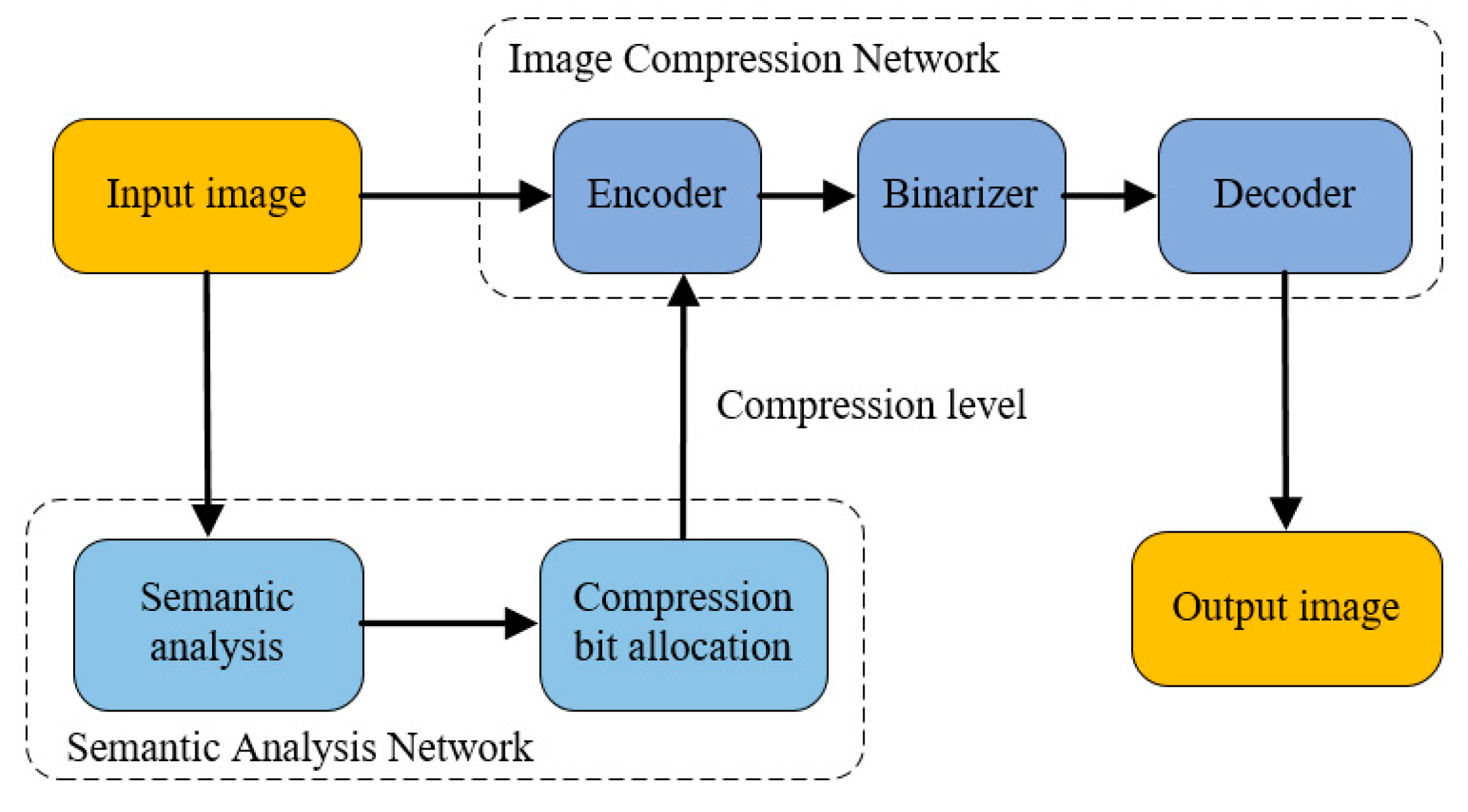
Figure 1. Compression framework.
Applsci 09 03580 g001
Figure 2. Semantic analysis network structure.
Applsci 09 03580 g002
Figure 3. Semantic importance map in Kodak.
Applsci 09 03580 g003
Figure 4. Compression network structure; “Conv (3,2,64)” is a convolution layer with 64 convolutional kernels, the kernel size is 3 × 3, the stride is 2 × 2. “LSTM A-1” is the long short-term memory (LSTM) unit A (from A to H) in iteration 1, and “Sp” is the sub-pixel structure.
Applsci 09 03580 g004
Figure 5. LSTM unit structure.
Applsci 09 03580 g005
Figure 6. Image produced by different compression methods at similar compression ratios. From the left to the right: original, JPEG, BPG, George’s, and ours. ‘B’ in multi-structure structural similarity (MS-SSIM)-B refers to the blue block, ‘G’ in MS-SSIM-G refers to the green block.
Applsci 09 03580 g006
Figure 7. Rate distortion curve on the Kodak dataset. SI-SSIM: proposed semantic–important structural similarity. (a) MS-SSIM index; (b) SI-SSIM index.
Applsci 09 03580 g007