A Bi-LSTM Based Ensemble Algorithm for Prediction of Protein Secondary Structure

Abstract
:1. Introduction
2. Materials and Performance Measure
2.1. Datasets
2.2. Performance Measure
3. Features and Methods
3.1. Features Selection
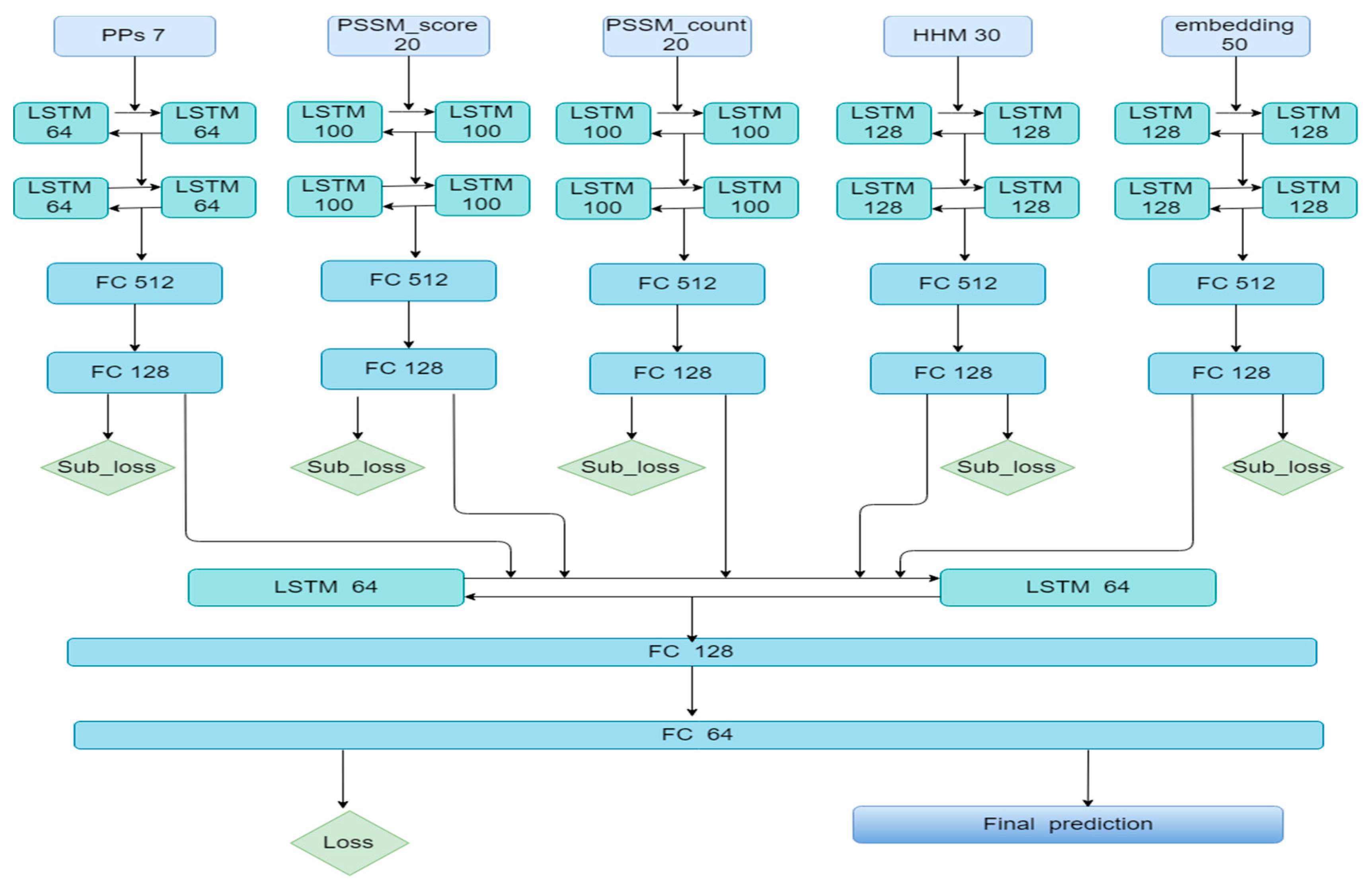
3.2. The Ensemble Algorithm Based on Bi-LSTM
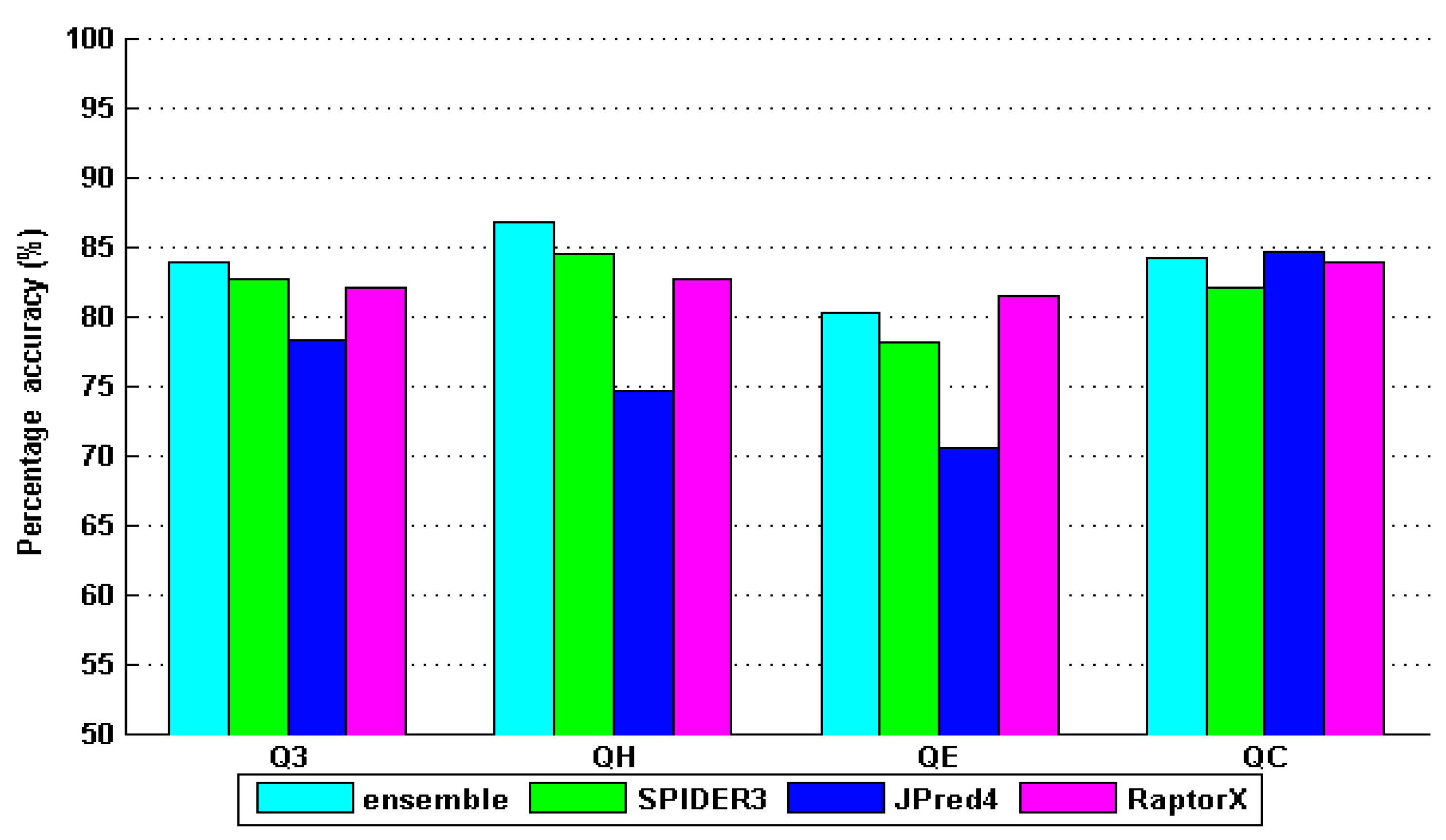
4. Results and Discussion
5. Conclusions
Author Contributions
Funding
Acknowledgments
Conflicts of Interest
Abbreviations
| LSTM | Long Short-Term Memory |
| PSSM | Position specific scoring matrix |
| Q3 | Overall accuracy |
| SOV | Segment overlap measure |
| MCC | Matthews correlation coefficient |
| PSI-BLAST | Position-Specific Iterative BLAST |
References
- Ward, J.J.; Mcguffin, L.J.; Buxton, B.F.; Jones, D.T. Secondary structure prediction with support vector machines. Bioinformatics 2003, 19, 1650–1655. [Google Scholar] [CrossRef]
- Xie, S.X.; Li, Z.; Hu, H.H. Protein secondary structure prediction based on the fuzzy support vector machine with the hyperplane optimization. Gene 2018, 642, 74–83. [Google Scholar] [CrossRef] [PubMed]
- Bondugula, R.; Xu, D. MUPRED: A tool for bridging the gap between template based methods and sequence profile based methods for protein secondary structure prediction. Proteins Struct. Funct. Bioinf. 2010, 66, 664–670. [Google Scholar] [CrossRef] [PubMed]
- Altschul, S.F.; Madden, T.L.; Schäffer, A.A.; Zhang, J.; Zhang, Z.; Miller, W.; Lipman, D.J. Gapped BLAST and PSI-BLAST: A new generation of protein database search programs. Nucleic Acids Res. 1997, 25, 3389–3402. [Google Scholar] [CrossRef] [PubMed]
- Geourjon, C.; Deléage, G. SOPM: A self-optimized method for protein secondary structure prediction. Protein Eng. Des. Sel. 1994, 7, 157–164. [Google Scholar] [CrossRef]
- Rost, B. Review: Protein secondary structure prediction continues to rise. J. Struct. Biol. 2001, 134, 204–218. [Google Scholar] [CrossRef] [PubMed]
- Yaseen, A.; Li, Y. Context-based features enhance protein secondary structure prediction accuracy. J. Chem. Inf. Model. 2014, 54, 992–1002. [Google Scholar] [CrossRef] [PubMed]
- Wang, S.; Peng, J.; Ma, J.; Xu, J. Protein secondary structure prediction using deep convolutional neural fields. Sci. Rep. 2016, 6, 18962. [Google Scholar] [CrossRef] [PubMed]
- Cortes, C.; Vapnik, V. Support-vector networks. Mach. Learn. 1995, 20, 273–297. [Google Scholar] [CrossRef]
- Karplus, K. SAM-T08, HMM-based protein structure prediction. Nucleic Acids Res. 2009, 37, 492–497. [Google Scholar] [CrossRef]
- Heffernan, R.; Paliwal, K.; Lyon, J.; Dehzangi, A.; Sharma, A.; Wang, J.; Sattar, A.; Yang, Y.; Zhou, Y. Improving prediction of secondary structure, local backbone angles, and solvent accessible surface area of proteins by iterative deep learning. Sci. Rep. 2015, 5, 11476. [Google Scholar] [CrossRef] [PubMed]
- Hochreiter, S.; Schmidhuber, J. Long short-term memory. Neural Comput. 1997, 9, 1735–1780. [Google Scholar] [CrossRef] [PubMed]
- Hinton, G.; Deng, L.; Yu, D.; George, E.; Mohamed, D.A.; Jaitly, N.; Senior, A.; Vanhoucke, V.; Nguyen, P.; Sainath, T.N.; et al. Deep neural networks for acoustic modeling in speech recognition: The shared views of four research groups. IEEE Signal Process. Mag. 2012, 29, 82–97. [Google Scholar] [CrossRef]
- Gal, Y.; Ghahramani, Z. A theoretically grounded application of dropout in recurrent neural networks. Adv. Neural Inf. Process. Syst. 2016, 285–290. [Google Scholar]
- Hanson, J.; Yang, Y.; Paliwal, K.; Zhou, Y. Improving protein disorder prediction by deep bidirectional long short-term memory recurrent neural networks. Bioinformatics 2017, 33, 685–692. [Google Scholar] [CrossRef] [PubMed]
- Kabsch, W.; Sander, C. Dictionary of protein secondary structure: Pattern recognition of hydrogen-bonded and geometrical features. Biopolym. Orig. Res. Biomol. 1983, 22, 2577–2637. [Google Scholar] [CrossRef] [PubMed]
- Rost, B.; Sander, C. Prediction of protein secondary structure at better than 70% accuracy. J. Mol. Biol. 1993, 232, 584–599. [Google Scholar] [CrossRef] [PubMed]
- Heffernan, R.; Yang, Y.; Paliwal, K.; Zhou, Y. Capturing non-local interactions by long short term memory bidirectional recurrent neural networks for improving prediction of protein secondary structure, backbone angles, contact numbers, and solvent accessibility. Bioinformatics 2017, 33, 2842–2849. [Google Scholar] [CrossRef]
- Clementi, C.; García, A.E.; Onuchic, J.N. Interplay among tertiary contacts, secondary structure formation and side-chain packing in the protein folding mechanism: All-atom representation study of protein L. J. Mol. Biol. 2003, 326, 933–954. [Google Scholar] [CrossRef]
- Matthews, B.W. Comparison of the predicted and observed secondary structure of T4 phage lysozyme. Biochim. Biophys. Acta 1975, 405, 442–451. [Google Scholar] [CrossRef]
- Zemla, A.; Venclovas, C.; Fidelis, K.; Rost, B. A modified definition of Sov, a segment-based measure for protein secondary structure prediction assessment. Proteins Struct. Funct. Bioinf. 1999, 34, 220–223. [Google Scholar] [CrossRef]
- Fauchère, J.L.; Charton, M.; Kier, L.B.; Verloop, A.; Pliska, V. Amino acid side chain parameters for correlation studies in biology and pharmacology. Int. J. Pept. Protein Res. 2010, 32, 269–278. [Google Scholar] [CrossRef]
- Remmert, M.; Biegert, A.; Hauser, A.; Söding, J. HHblits: Lightning-fast iterative protein sequence searching by HMM-HMM alignment. Nat. Methods 2012, 9, 173–175. [Google Scholar] [CrossRef]
- Levy, O.; Goldberg, Y. Neural word embedding as implicit matrix factorization. Adv. Neural Inf. Process. Syst. 2014, 3, 2177–2185. [Google Scholar]
- Salvatore, M.; Warholm, P.; Shu, N.; Basile, W.; Elofsson, A. SubCons: A new ensemble method for improved human subcellular localization predictions. Bioinformatics 2017, 33, 2464–2470. [Google Scholar] [CrossRef] [PubMed]
- Li, Z.; Wang, J.; Zhang, S.; Zhang, Q.; Wu, W. A new hybrid coding for protein secondary structure prediction based on primary structure similarity. Gene 2017, 618, 8–13. [Google Scholar] [CrossRef] [PubMed]
- Murakami, Y.; Mizuguchi, K. Applying the Naïve Bayes classifier with kernel density estimation to the prediction of protein–protein interaction sites. Bioinformatics 2010, 26, 1841–1848. [Google Scholar] [CrossRef] [PubMed]
- Srivastava, N.; Hinton, G.; Krizhevsky, A.; Sutskever, I.; Salakhutdinov, R. Dropout: A simple way to prevent neural networks from overfitting. J. Mach. Learn. Res. 2014, 15, 1929–1958. [Google Scholar]
- Kingma, D.; Ba, J. Adam: A method for stochastic optimization. Comput. Sci. 2014, arXiv:1412.698012. [Google Scholar]
- Pascanu, R.; Mikolov, T.; Bengio, Y. On the difficulty of training recurrent neural networks. Int. Conf. Mach. Learn. 2013, 1310–1318. [Google Scholar]
- Drozdetskiy, A.; Cole, C.; Procter, J.; Barton, G.J. JPred4: A protein secondary structure prediction server. Nucleic Acids Res. 2015, 43, 389–394. [Google Scholar] [CrossRef] [PubMed]
- Wang, S.; Li, W.; Liu, S.; Xu, J. RaptorX-Property: A web server for protein structure property prediction. Nucleic Acids Res. 2016, 44, 430–435. [Google Scholar] [CrossRef] [PubMed]
- Hanson, J.; Paliwal, K.; Litfin, T.; Yang, Y.; Zhou, Y. Improving prediction of protein secondary structure, backbone angles, solvent accessibility, and contact numbers by using predicted contact maps and an ensemble of recurrent and residual convolutional neural networks. Bioinformatics 2018, 35, 2403–2410. [Google Scholar] [CrossRef] [PubMed]
- Bahdanau, D.; Cho, K.; Bengio, Y. Neural machine translation by jointly learning to align and translate. Comput. Sci. 2014, arXiv:1409.04739. [Google Scholar]


| Methods | Accuracy Measures | ||||||
|---|---|---|---|---|---|---|---|
| SOV (%) | SOVH (%) | SOVE (%) | SOVC (%) | CH | CE | CC | |
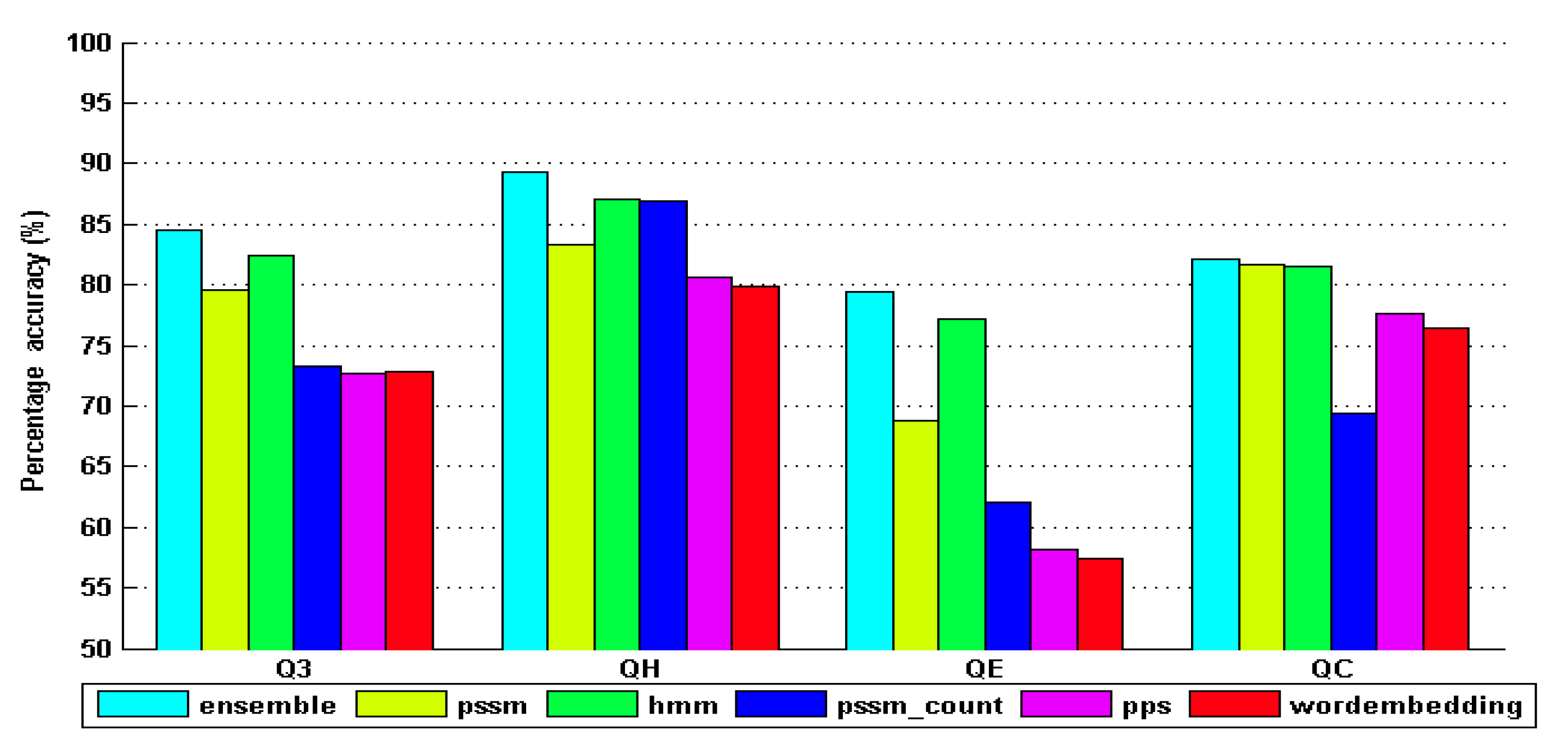
| ensemble_model | 81.917 | 86.468 | 82.289 | 77.382 | 0.838 | 0.769 | 0.697 |
| pssm_model | 74.482 | 76.246 | 70.825 | 72.112 | 0.761 | 0.693 | 0.642 |
| hmm_model | 80.138 | 83.086 | 79.831 | 75.512 | 0.796 | 0.782 | 0.682 |
| pssm_c_model | 64.831 | 71.456 | 58.314 | 61.087 | 0.656 | 0.589 | 0.537 |
| pps_model | 64.821 | 68.257 | 56.752 | 65.251 | 0.648 | 0.572 | 0.542 |
| wordem_model | 64.785 | 66.721 | 56.543 | 63.563 | 0.653 | 0.558 | 0.562 |
| Methods | Accuracy Measures | ||||||
|---|---|---|---|---|---|---|---|
| SOV (%) | SOVH (%) | SOVE (%) | SOVC (%) | CH | CE | CC | |
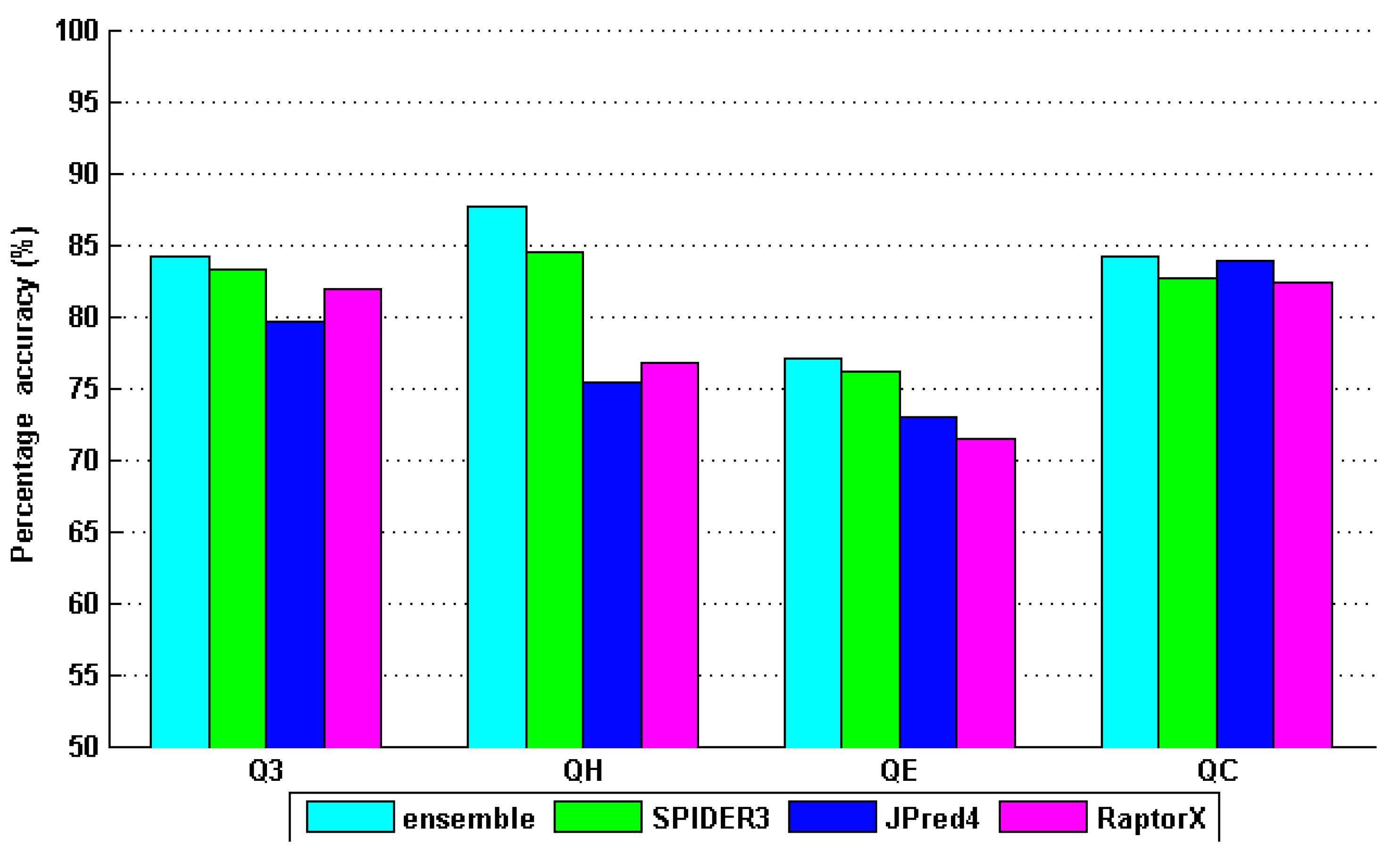
| ensemble | 81.56 | 85.69 | 84.38 | 76.57 | 0.8059 | 0.7917 | 0.6862 |
| SPIDER3 | 80.90 | 87.50 | 81.40 | 73.70 | 0.7905 | 0.7518 | 0.6524 |
| JPred4 | 70.90 | 77.90 | 74.20 | 64.10 | 0.7236 | 0.6771 | 0.5891 |
| RaptorX | 76.50 | 81.00 | 80.40 | 71.20 | 0.7833 | 0.7375 | 0.6515 |
| Methods | Accuracy Measures | ||||||
|---|---|---|---|---|---|---|---|
| SOV (%) | SOVH (%) | SOVE (%) | SOVC (%) | CH | CE | CC | |
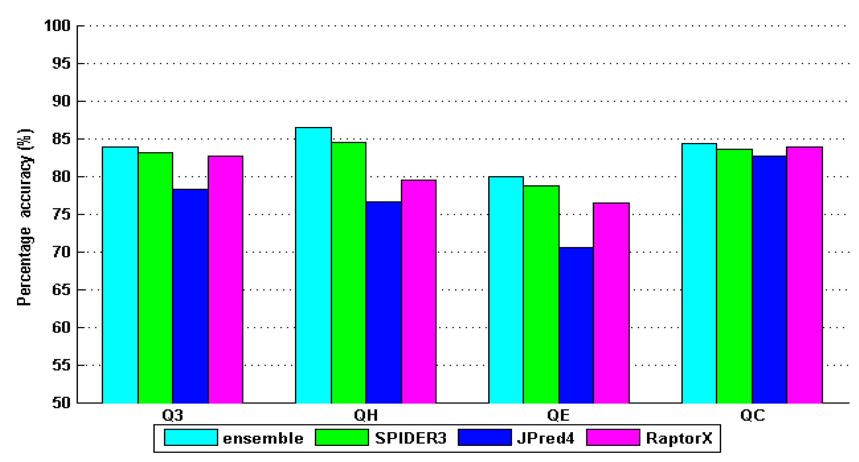
| ensemble | 80.50 | 84.70 | 83.20 | 75.80 | 0.8052 | 0.7964 | 0.6942 |
| SPIDER3 | 77.90 | 83.50 | 79.40 | 72.70 | 0.7905 | 0.7518 | 0.6524 |
| JPred4 | 70.90 | 77.90 | 74.20 | 64.10 | 0.7236 | 0.6771 | 0.6291 |
| RaptorX | 76.50 | 81.00 | 80.40 | 71.20 | 0.7833 | 0.7675 | 0.6735 |
| Methods | Accuracy Measures | ||||||
|---|---|---|---|---|---|---|---|
| SOV (%) | SOVH (%) | SOVE (%) | SOVC (%) | CH | CE | CC | |
| ensemble | 80.60 | 84.50 | 82.60 | 75.45 | 0.8058 | 0.7854 | 0.6977 |
| SPIDER3 | 78.10 | 83.20 | 79.20 | 72.50 | 0.7978 | 0.7126 | 0.6721 |
| JPred4 | 72.20 | 76.80 | 75.10 | 64.60 | 0.7324 | 0.6796 | 0.6043 |
| RaptorX | 75.40 | 80.80 | 82.30 | 71.20 | 0.7839 | 0.7598 | 0.6757 |
© 2019 by the authors. Licensee MDPI, Basel, Switzerland. This article is an open access article distributed under the terms and conditions of the Creative Commons Attribution (CC BY) license (http://creativecommons.org/licenses/by/4.0/).
Share and Cite
Hu, H.; Li, Z.; Elofsson, A.; Xie, S. A Bi-LSTM Based Ensemble Algorithm for Prediction of Protein Secondary Structure. Appl. Sci. 2019, 9, 3538. https://doi.org/10.3390/app9173538
Hu H, Li Z, Elofsson A, Xie S. A Bi-LSTM Based Ensemble Algorithm for Prediction of Protein Secondary Structure. Applied Sciences. 2019; 9(17):3538. https://doi.org/10.3390/app9173538
Chicago/Turabian StyleHu, Hailong, Zhong Li, Arne Elofsson, and Shangxin Xie. 2019. "A Bi-LSTM Based Ensemble Algorithm for Prediction of Protein Secondary Structure" Applied Sciences 9, no. 17: 3538. https://doi.org/10.3390/app9173538
APA StyleHu, H., Li, Z., Elofsson, A., & Xie, S. (2019). A Bi-LSTM Based Ensemble Algorithm for Prediction of Protein Secondary Structure. Applied Sciences, 9(17), 3538. https://doi.org/10.3390/app9173538