Article

LSTM DSS Automatism and Dataset Optimization for Diabetes Prediction †

Dyrecta Lab srl, Via Vescovo Simplicio 45, 70014 Conversano, Italy
*
Author to whom correspondence should be addressed.
This work is an extended version of our research published in 2018 at the conference “AEIT 2018 International Annual Conference” held in Bari, Italy, 3–5 October 2018.
Appl. Sci. 2019, 9(17), 3532; https://doi.org/10.3390/app9173532
Submission received: 28 June 2019 / Revised: 19 August 2019 / Accepted: 21 August 2019 / Published: 28 August 2019

Abstract

:

Featured Application

Implementation of DSS of patient management system based on LSTM for homecare assistance.

Abstract

The paper is focused on the application of Long Short-Term Memory (LSTM) neural network enabling patient health status prediction focusing the attention on diabetes. The proposed topic is an upgrade of a Multi-Layer Perceptron (MLP) algorithm that can be fully embedded into an Enterprise Resource Planning (ERP) platform. The LSTM approach is applied for multi-attribute data processing and it is integrated into an information system based on patient management. To validate the proposed model, we have adopted a typical dataset used in the literature for data mining model testing. The study is focused on the procedure to follow for a correct LSTM data analysis by using artificial records (LSTM-AR-), improving the training dataset stability and test accuracy if compared with traditional MLP and LSTM approaches. The increase of the artificial data is important for all cases where only a few data of the training dataset are available, as for more practical cases. The paper represents a practical application about the LSTM approach into the decision support systems (DSSs) suitable for homecare assistance and for de-hospitalization processes. The paper goal is mainly to provide guidelines for the application of LSTM neural network in type I and II diabetes prediction adopting automatic procedures. A percentage improvement of test set accuracy of 6.5% has been observed by applying the LSTM-AR- approach, comparing results with up-to-date MLP works. The LSTM-AR- neural network can be applied as an alternative approach for all homecare platforms where not enough training sequential dataset is available.

Graphical Abstract

1. Introduction

A research topic in telemedicine is the predictive diagnostic improved by artificial intelligence (AI). Different open source tools [1,2,3,4] such as RapidMiner Studio, Weka, Konstanz Information Miner (KNIME), Orange Canvas, Keras, TensorFlow, and Theano can be applied for this purpose, implementing generic artificial neural networks (ANN) predicting patient health status. These tools are suitable for decision support systems (DSS) based on artificial intelligence algorithms [5,6,7,8,9,10,11,12,13] predicting diagnosis [14,15,16]. Specifically in references [5,6,10,11,12,13] are discussed how data mining could support hospital and assistance processes, while references [7,8,9,14,15,16] provide different healthcare applications where artificial intelligence plays an important role in decision making processes enabled by health status prediction. Accordingly, with homecare assistance facilities for de-hospitalization processes, the use of certified smart sensors transmitting data in a cloud network could remotely control the patients at home [17]. The sensor enabling homecare assistance can be implemented into a more complex information hospital system embedding automatic alerting conditions based on different risk levels [18]. In this direction, KNIME workflows can be easily interfaced as a Graphical User Interface (GUI) to the control room information system, thus allowing the connectivity with big data systems and timing data process by cron job run managing the multilayer perceptron (MLP) ANN analyses [19]. In Figure 1a is illustrated an example information system basic architecture of the MLP ANN network linked with the control room and big data system for homecare assistance [19], and in Figure 1b schematized the related KNIME workflow by distinguishing the data process phases such as time delay for the workflow execution, python node enabling data input access, data pre-processing, data model processing, and reporting [19].
The ANN model implemented by workflows with objects are user friendly but cannot be easily implemented into Enterprise Resource Planning (ERP) software. For this purpose it is preferable to embed ANN scripts directly into the ERP framework, thus facilitating the DSS platform implementation and execution. For this purpose, it is preferable to adopt the python language, which can be easily embedded in different ERP frameworks. In previous literature the Long Short-Term Memory (LSTM) neural network has been adopted for predictive diagnostics, assuring good performance results [20,21,22]. Following this direction, the traditional ANN MLP prediction network, applied in the work [19] using a single attribute labeling, has been substituted by an LSTM neural network based on a multi-attribute analysis. The passage from the workflow implementation to the python script is necessary in order to properly design a neural network embedded into an ERP platform, potentially enabling data processing automatisms. In order to check the performance of the upgraded network has been processedt the experimental dataset of [23,24], representing a good dataset for testing LSTM neural network. The experimental dataset [24] has been adopted in the literature for different data mining testing [24,25,26,27,28,29]. Specifically in reference [25], the K-means algorithm has been applied for predicting diabetes, in reference [26] some authors applied synthetic data in order to balance a machine learning dataset model, while references [27,28,29] have analyzed different machine learning algorithms for diabetes prediction.
Concerning data mining algorithms, some researchers focused their attention on the formulation of decision tree models for Type 2 Diabetes Mellitus (T2DM) [30]. Other studies analyzed the sensitivity of Machine Learning Algorithms about self-monitored blood glucose (SMBG) readings [31], thus enhancing the importance to construct a good learning model. The Deep Learning Approach has also been adopted for the prediction of blood glucose levels [32]. Furthermore, data mining algorithms can be applied for prediction and prevention of complications associated with diabetes [33,34]. According to the World health Organization, the number of people with diabetes has risen from 108 million in 1980 to 422 million in 2014, respectively. For this reason, a good DSS could support diagnostic prediction, thus facilitating diabetes care.
This paper developed an LSTM neural network suitable for DSS platforms, upgrading the architecture of Figure 1 by adding the following specifications:
-
LSTM python script enabling software verticalization and integration in ERP platforms oriented on patient management;
-
Integration of LSTM neural network into the information system collecting patient information and patient data;
-
Creation of different data models allowing data pre-processing and new facilities oriented on patient management;
-
Creation of a prediction model based on the simultaneous analysis of multiple attributes;
-
Adoption of artificial data in order to improve the training dataset;
-
Possibility to choose the best prediction models by reading different model outputs.

2. Materials and Methods

Based on several studies, we found that a commonly used dataset for health data mining was the Pima Indians Diabetes Dataset from the University of California, Irvine (UCI) Machine Learning Database [24,25,26,27,28,29]. The datasets consist of several medical predictor (independent) variables and one target (dependent) variable, Outcome. Independent variables include the number of pregnancies the patient has had, their BMI, insulin level, age, and so on:
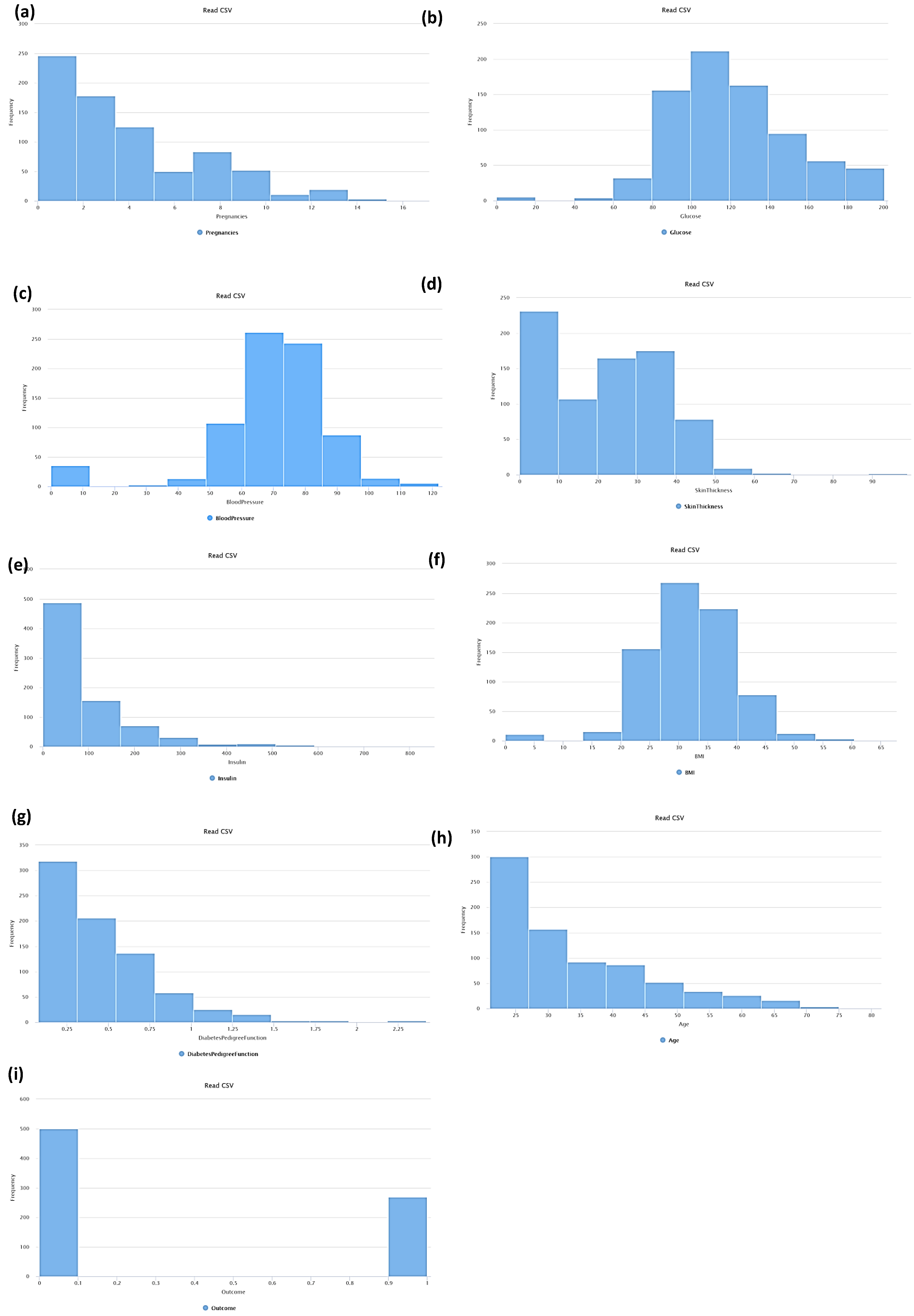
  • PregnanciesNumber (PN): Pregnant number;
  • GlucosePlasma (GP): Glucose concentration (after 2 h of oral glucose tolerance test);
  • BloodPressureDiastolic (BPD): Blood pressure (mm Hg);
  • SkinThicknessTriceps (STT): Skin fold thickness (mm);
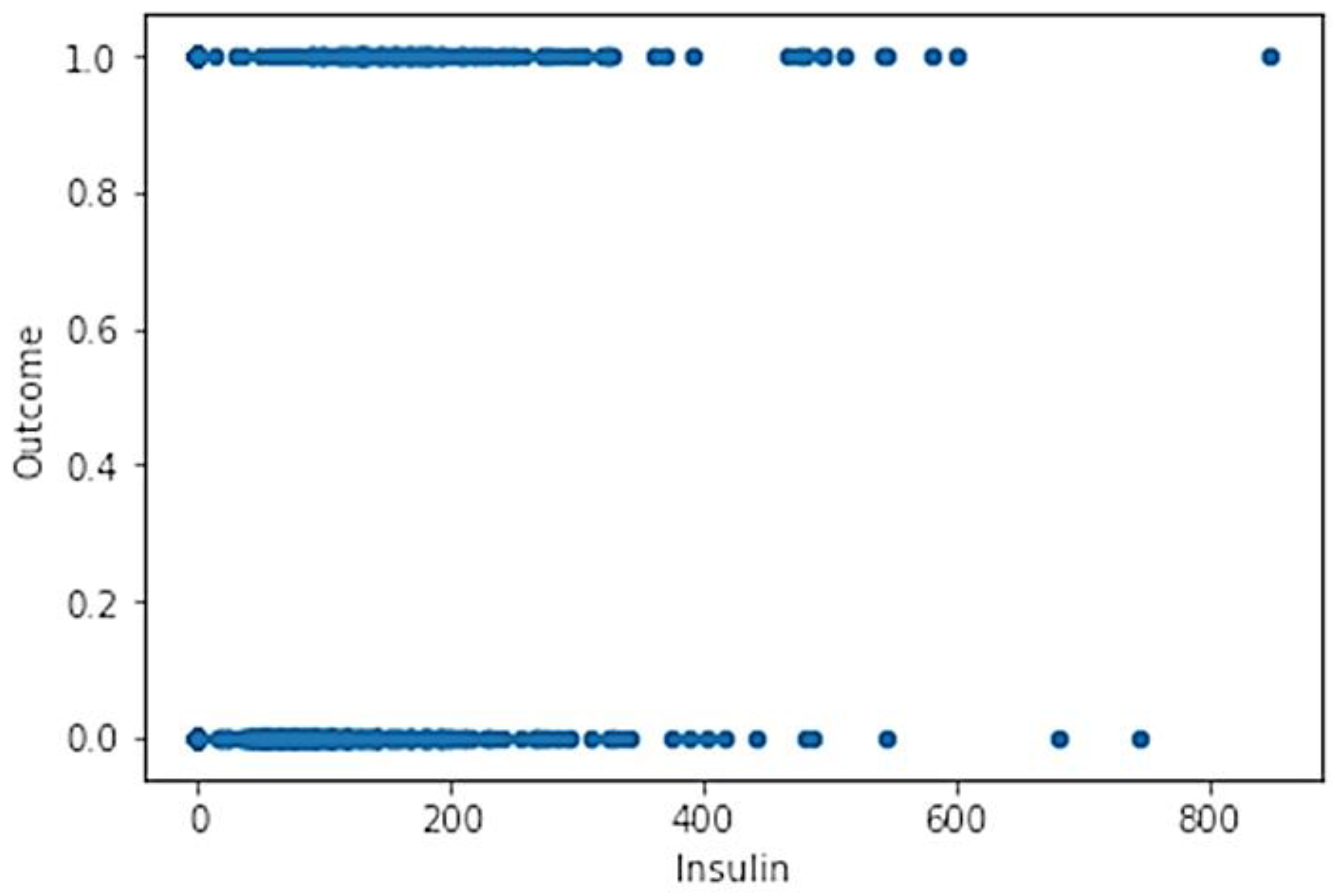
  • Insulin2-Hour (I): Serum insulin (mu U/mL);
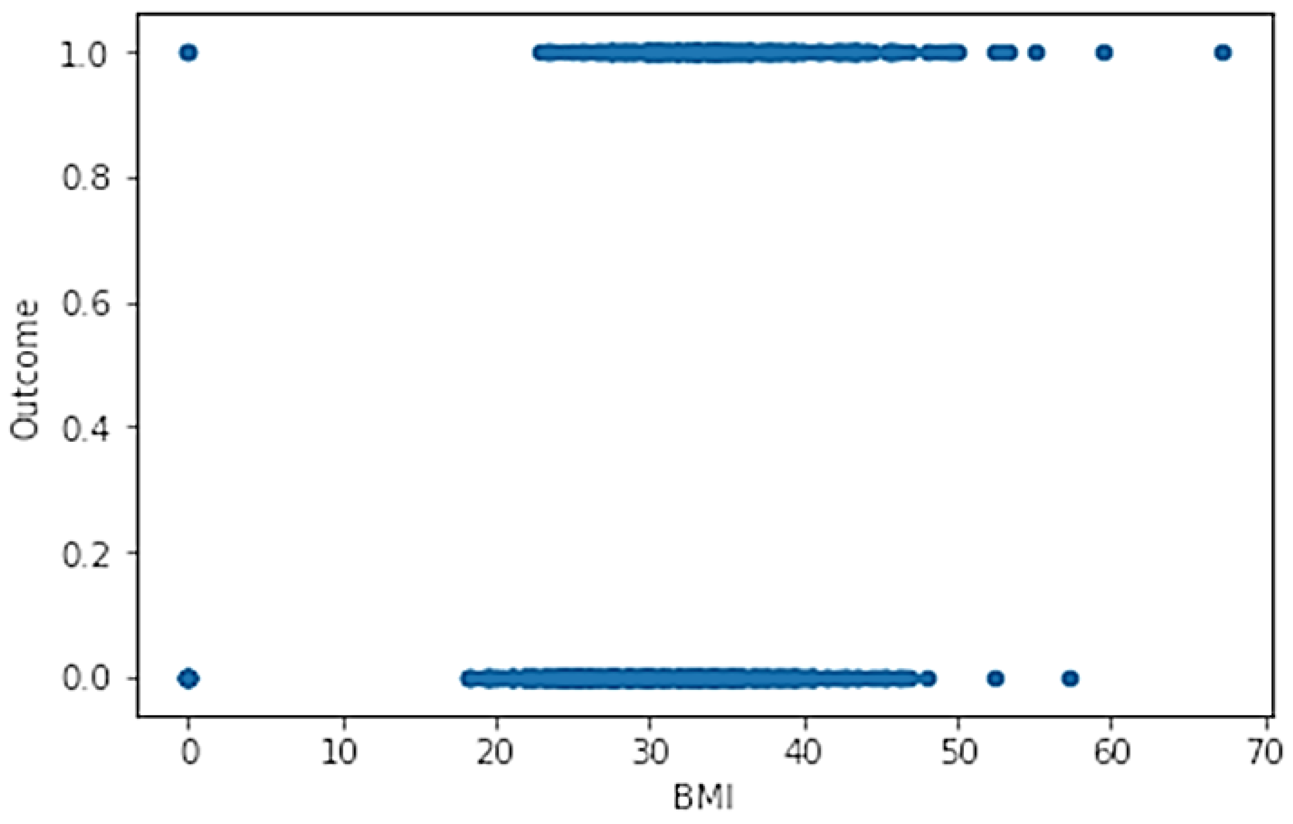
  • BMIBody (BMI): Mass index (weight in kg/(height in m)2);
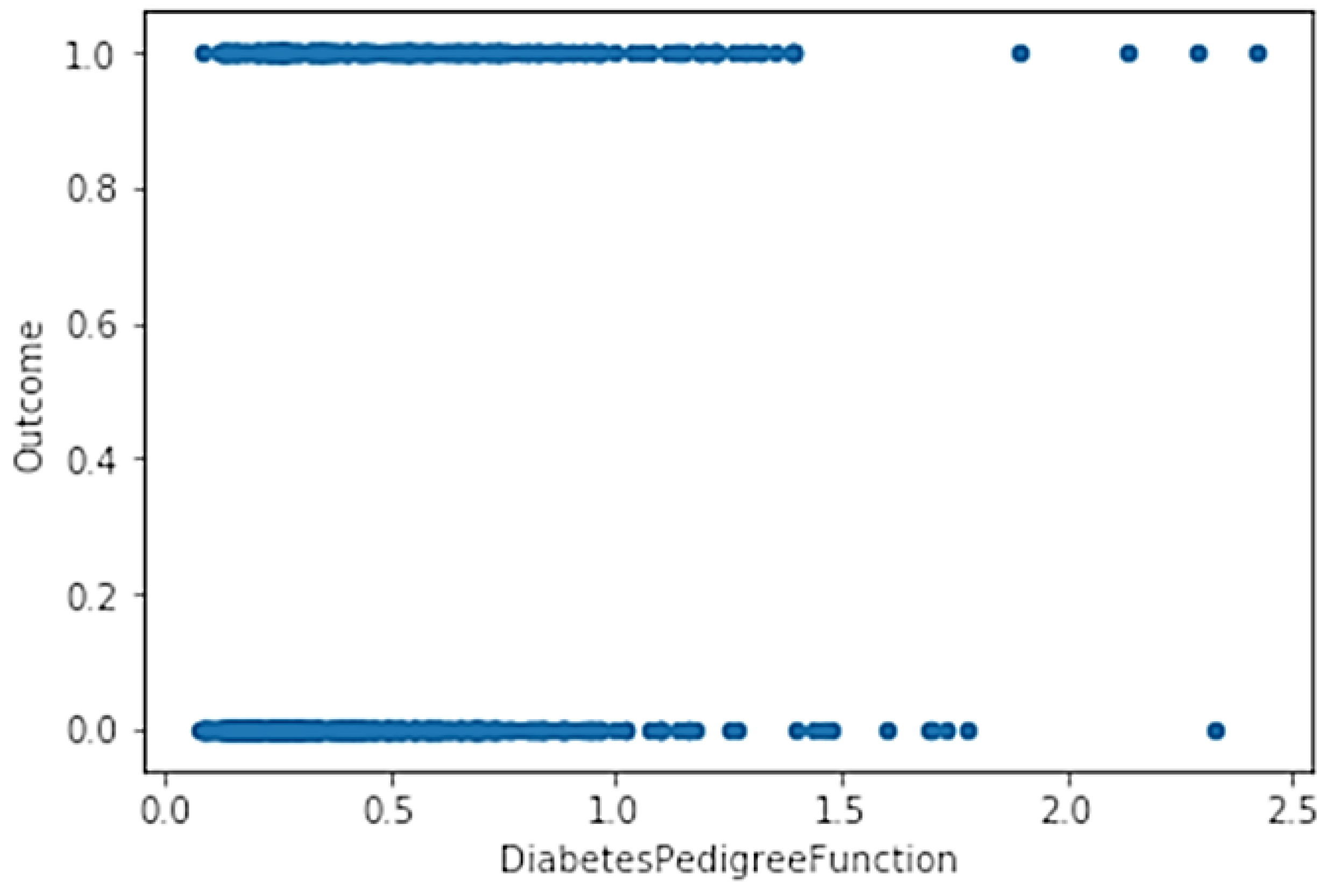
  • DiabetesPedigreeFunctionDiabetes (DPFD): Pedigree function;
  • AgeAge (AA): Years old;
  • OutcomeClass (OC): Binary variable (0 indicates the no-diabetes status of 268 samples, and 1 indicates the diabetes status of the remaining 500 cases of the training dataset).
In Figure 2 is illustrated the statistic distribution of the above listed attributes plotted by RapidMiner tool.
In general, before processing data by data mining algorithms, it is important to analyze the correlation between attributes in order to choose the less correlated variables: By processing strong correlated variables, which can be introduced into the system redundancies and calculus sensitivities, which can alter the results and increase the data process error or the prediction error. These considerations are valid also for LSTM processing. A method to estimate the correlation between variables generating a weights vector based on these correlations is Pearson’s correlation coefficient evaluation. The algorithm calculates this coefficient, which is the covariance of the two variables divided by the product of their standard deviations [35,36]:
ρ X , Y = c o v ( X , Y ) σ X σ Y
being Cov (X,Y), the covariance of the variables X and Y (σXY), and σX and σY the standard deviation of variable X and Y, respectively.
By observing the calculated correction matrix of Table 1 (data processing of the experimental dataset) it is clear that all the attributes are not strongly correlated.
A first check of correlation can also be performed by directly observing the 2D plots between a couple of variables. By focusing the attention on the OutcomeClass variable indicating diabetic status, it was evident from Figure 3, Figure 4 and Figure 5 that generally the classes 1 and 0 were not distinguished in the function of the other variables (data overlapping). This confirmed that the results found in the correlation matrix and provided information about samples dispersion.
The prediction results about the outcome variable (labeled variable) were performed by the LSTM neural network. The LSTM basic architecture [37] was composed of a cell, an input gate, an output gate, and a forget gate. Each cell recalled values over arbitrary time intervals, besides the 3 gates regulated the flow of information into and out of the cell. In Figure 6 it has ditched a scheme of the LSTM neural network cell where the input (input activation at the time step t it), output (output activation at the time step t ot), and forget (forget activation at the time step t ft) gates behaved as neuron computing in a feed-forward or multi-layer neural network: The gates calculated their activations at time step t by considering the activation of the memory cell C at time step t-1. More details about the LSTM neural network models are in the script comments of Appendix A.
The output parameters indicating the LSTM performance are the model accuracy, the model loss and the Receiver Operating Characteristic (ROC) curve indicating the Area under the ROC Curve—AUC—(performance indicator). Loss value defines how well the LSTM neural network model behaves after each iteration of optimization (ideally, one would expect the reduction of loss after each, or several, iterations). The accuracy parameter is defined as:
A c c u r a c y = N u m b e r   o f   c o r r e c t   p r e d i c t i o n s T o t a l   n u m b e r   o f   p r e d i c t i o n s = T P + T N T P + T N + F P + F N
being TP = True Positives, TN = True Negatives, FP = False Positives, and FN = False Negatives.
The loss function is a binary cross-entropy used for the problems involving yes/no (binary) decisions. For instance, in multi-label problems, where an example can belong simultaneously to multiple classes, the model tries to decide for each class whether the example belongs to that class or not. This performance indicator is estimated as:
L o s s ( y , y p ) = 1 N i = 0 N ( y log ( y p ) + ( 1 y ) log ( 1 y p ) )
where yp is the predicted value.
As calculation tools have been adopted Keras API and TensorFlow library: Keras is a high-level API suitable for building and training deep learning models (LSTM), and TensorFlow is a free and open-source software library for dataflow and differentiable programming across a range of tasks.

3. Results

In this section are shown the LSTM neural network results by enhancing some aspects of model consistency in function of the training and testing dataset percentage used for the calculation.

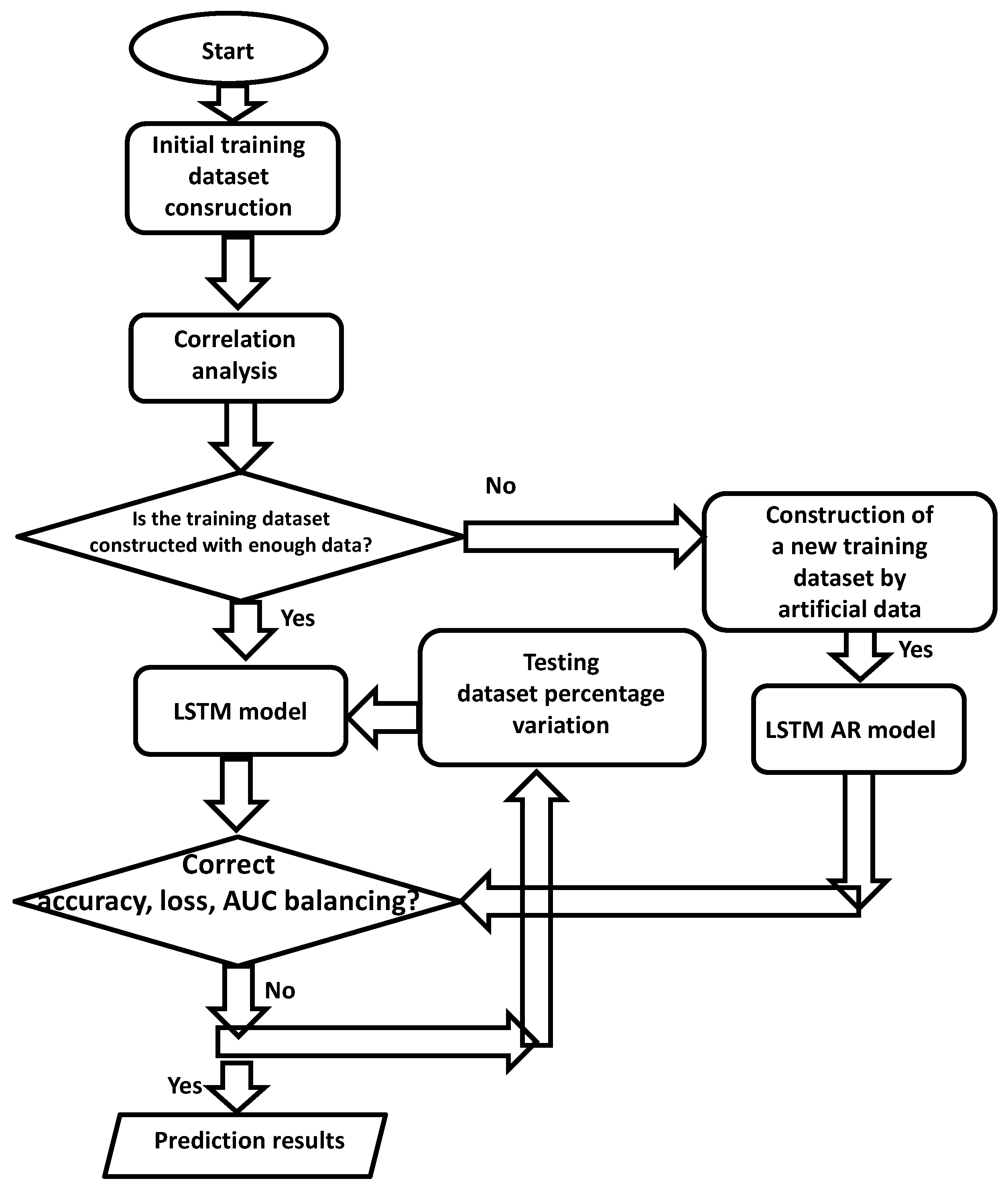
Training and Testing Dataset

The training and the testing dataset were randomly extracted from the whole dataset made by 768 records. This allows a decrease in the error calculation of the LSTM network by limiting data redundancy and consecutively data correlation and sensitivity. Table 2 illustrates a table extracted from output results indicating the diabetic outcome prediction, where the predicted OC is the output and the other listed variables are the input testing attributes.
In order to estimate, the outcome prediction has been applied to the LSTM neural network by changing the partitioning between experimental and training dataset. Different calculations have been performed by changing the testing dataset percentage. In particular, Figure 7, Figure 8, Figure 9, Figure 10 and Figure 11 illustrate the accuracy the losses and the ROC curve of the case of testing dataset percentage of 5%, 10%, 15%, 20%, and 25%, respectively.
The best convergence was observed for the model accuracy of Figure 10, thus confirming that a good balancing between test and train model was achieved (case of testing dataset of 20%). Evident overfitting was observed in the model accuracy of Figure 9 related to 15% of testing dataset (no good balancing of parameters).
From the ROC curves can be calculated the AUC values.
Summarized in Table 3 are the results of the AUC, accuracy, and loss of the adopted models, where the green color indicates a better result.
The red and the green colors refer to values above or below thresholds considered valid for LSTM outputs. Specifically, the following thresholds have been considered: 86% for AUC %, 75% for the accuracy, and 60% for loss. The thresholds could be integrated into an automatic procedure able to select the best model to apply.
In Appendix A is listed the python script used for the testing.
The LSTM approach has been improved by implementing a new approach to the training dataset construction based on artificial data creation (LSTM artificial records—AR—). In the case of 20% of the testing dataset characterized by the best compromise between accuracy and loss parameter has created a new training dataset following these criteria:
-
Choose the attributes characterized by a higher correlation if compared with other attributes (in the case of study are insulin correlated with glucose, and skin thickness correlated with BMI);
-
Split the dataset for patients having diabetes or not (first partition);
-
The first partition has been furthermore split by considering the age (second partition);
-
The second partition is then split into a third one representing pregnant women (third partition);
-
Change of the correlated attributes by a low quantity of the values couple glucose and insulin (by increasing insulin is decreased the glucose of the same entity in order to balance the parameter variation), and skin thickness and BMI of the same person belonging to the same partition.
The goal of the proposed criteria is to generate artificial records improving the training dataset stability and test accuracy. The increase in artificial data is important for all cases where only few data of the training dataset are available, as for more practical cases.
In the case of this study, a training dataset has been created of 10,000 records, where only 768 are real.
The cross validation has been performed on MLP traditional methods, and on LSTM using artificial records—AR—(LSTM-AR-). In Table 4 a benchmarking performed by the comparison of the test set accuracy parameter is provided between traditional MLP [38], LSTM traditional algorithm, and the innovative LSTM-AR-approach.
Observing the comparison, it is evident an efficiency increase of the LSTM-AR- of 9% if compared with the LSTM traditional approach, and of 6.5% if compared with the MLP method optimized for diabetes prediction model [38]. Figure 12, Figure 13 and Figure 14 illustrate the accuracy, the loss, and the ROC curve of the LSTM-AR- outputs.
In particular, the model accuracy of Figure 12 proves that a good parameter balancing is achieved in terms of convergence, and no overfitting is observed.
Table 5 reports the comparison between the traditional LSTM approach and LSTM-AR- one, where it is observed that there is an efficiency improvement performed by LSTM-AR-.

4. Discussion

The proposed results allow us to define guidelines to adopt for LSTM data processing in general for data analysis in health applications using a generic dataset. The main steps are summarized as follows:
-
Calculation of correlation matrix (analysis of correlation and weights between variables);
-
Check of 2D variable functions (check of samples dispersion);
-
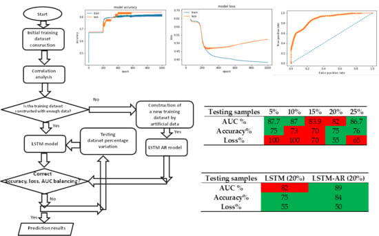
Calculation of LSTM prediction of diabetic outcomes by changing the partitioning between the testing and the training dataset;
-
Choice procedures of the best LSTM model.
In order to apply correctly the LSTM, one approach is to balance both the indicators loss and accuracy. By observing Table 3, the case of the training dataset of 20% represents a good case of this balancing but allows a relative low AUC value if compared with the other cases. For this purpose, it is important to compare the outputs of the model with the case of good AUC performance related to the cases of testing samples of 5%, 10%, and 25%. This “cross comparison” will facilitate a better understanding of which samples can be classified in false positive or false negative classes. Observing correlation matrix results of Table 1, we note that GlucosePlasma (GP) and OutcomeClass (OC) are correlated by a factor of 0.47, and PregnanciesNumber (PN) and AgeAge (AA) are correlated by a factor 0.57. For this purpose, these attributes could contribute negatively to the model convergence and for AUC values. In other dataset cases, the correlations between attributes can be stronger by adding further complexity to the LSTM output analysis. For this reason, it is important to compare the results of different models in order to find the best reading procedure involving:
-
The extraction of outliers related to wrong measurements and to neglect from the training and testing dataset;
-
The combined analysis of the therapeutic plan of the monitored patient;
-
The analysis of possible failures of the adopted sensors;
-
A dynamical update of the training model by changing anomalous data records;
-
The digital traceability of the assistance pattern in order to choose a patient more suitable to construct the training model;
-
A pre-clustering of patients (data pre-processing performed by combining different attributes such as age, pathology, therapeutic plan, etc.).
We note that in medical and clinical analysis the AUC is considered as a classifier able to discriminate the capacity of a test (see Table 6) [39]. All the AUC values found during the test are classified as “moderately accurate test”. In addition, for this reason, it is important to focus the attention on the convergence between Loss and Accuracy parameters.
The sensitivity of the LSTM neural network is then correlated with the specific used model and with the choosen dataset. The possibility to find common data patterns is then important to formulate a correct training dataset.
The goal is to perform a preliminary cross-analysis by considering all the patient information, which are collected into a database system (see Appendix B representing the adopted experimental database). The cross-analysis will contribute to creating the best LSTM training model. A good procedure to follow is:
-
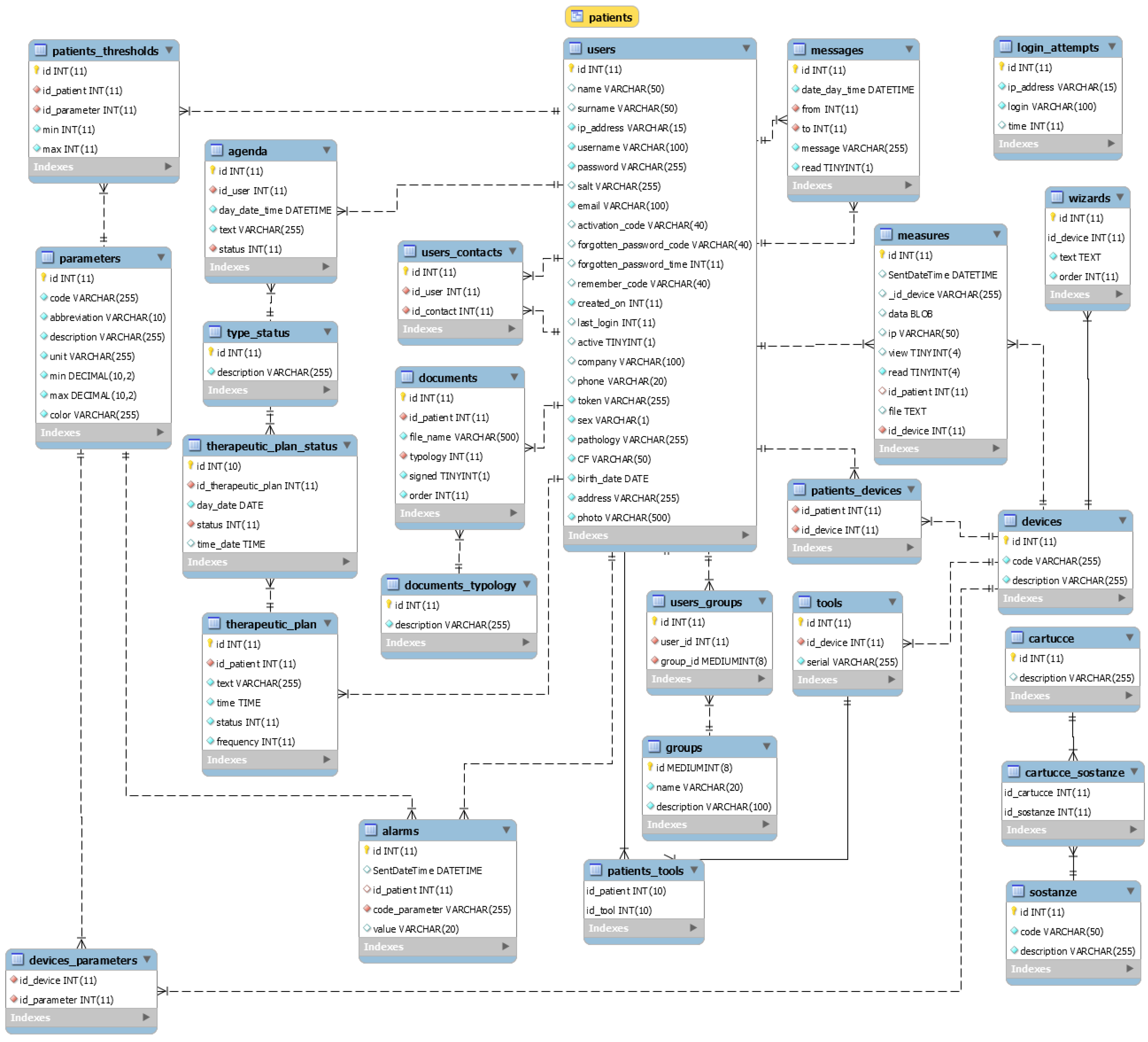
Phase 1: Collecting patient data (by means of a well-structured database system allowing different data mining processing);
-
Phase 2: Pre-clustering and filtering of patient data (construction of a stable training dataset);
-
Phase 3: Pre-analysis of correlations between attributes and analysis of data dispersions;
-
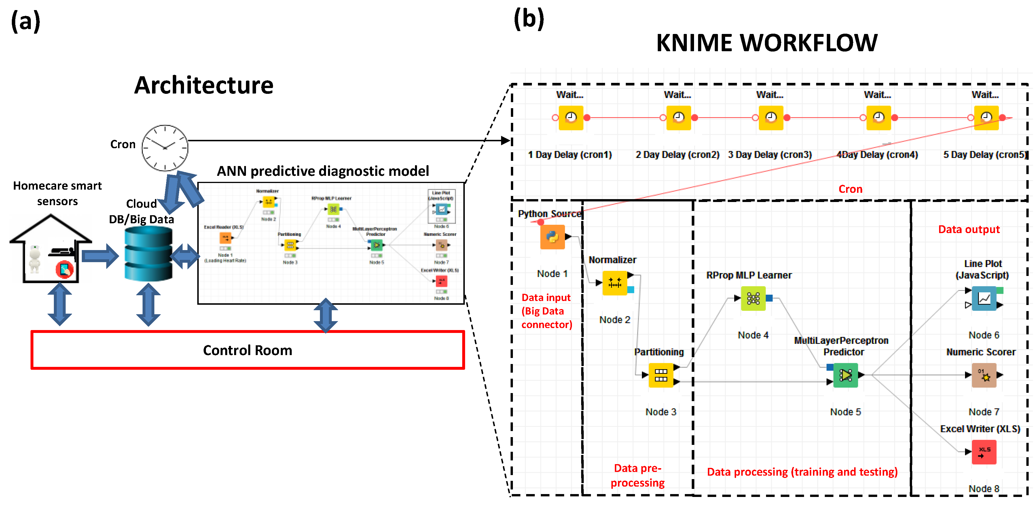
Phase 4: Execution of the LSTM neural network algorithm by processing simultaneously different attributes (multi-attribute data processing);
-
Phase 5: Comparison of results by changing the testing dataset;
-
Phase 6: Choice of the best model to adopt following the analysis of phase 5.
We observe that by repeating the calculation of the random testing datasets, same range values are obtained of the plots of Figure 8, Figure 9, Figure 10, Figure 11, Figure 12, Figure 13, Figure 14 and Figure 15, thus confirming the validity of the result discussion.
The limitations and advantages of the proposed study are summarized in the following Table 7:
Concerning dataset optimization has increased the LSTM performances by adding artificial data into the training dataset by defining the DSS automatism represented by the flow chart of Figure 15: The LSTM neural network model is applied automatically when the training dataset is constructed with enough data, otherwise a new training dataset will be formulated by artificial data (LSTM-AR- model) following the criteria discussed in Section 3. The flowchart of Figure 15 summarizes all the concepts discussed in this paper.
In order to test the LSTM-AR- algorithm on a time series dataset has been considered the sequential dataset of reference [40] (9086 time series data generated by 70 patients). This dataset is suitable for many architectures related to homecare smart assistance platforms.
By observing the results of Table 8, it is clear that LSTM and LSTM-AR- approaches are characterized by the same performances. In particular LSTM and the LSTM-AR- exhibit a percentage improvement of Accuracy and Loss of 4% if compared with MLP results.
In this case, the artificial records (454,300 artificial records) have been created by considering the sequential dataset by extracting sub- data set sequences with traditional sliding window approach. The MLP network is optimized for the new performed test (1 hidden layer enabling 30 neurons). Appendix C indicates the adopted MLP network. The adopted LSTM is the recurrent neural network—RNN—described in Appendix A (where sequential datasets will not be considered in structure reshaping).
In this last case, the selected epochs number is 200 because over 200 there was no performance improvement. Figure 16 and Figure 17 illustrate two graphs proving this cross validation method [41]. For all the other cases, the choice of the epochs number followed the same criterion.
The illustrated outputs are the average result of 25 trainings.
As observed in Table 6, the LSTM-AR- approach is characterized by the same performance of the LSTM method by confirming that it is suitable for all homecare platforms where not enough in the training sequential dataset is available.

5. Conclusions

The proposed paper shows how important the data sensitivity analysis in LSTM diabetes is, and predictions also considered patient attributes characterized by low correlations. The high sensitivity is mainly due to the creation of the training and testing dataset. The research is focused on the sensitivity analysis versus the testing dataset partitioning, by means of a stable experimental dataset tested in the literature. Following the performed analysis, a useful guideline to execute correct data processing and analysis by means of the LSTM neural network algorithm, processing different patient attributes, has been formulated. The discussion is mainly focused on the simultaneous analysis and comparison of the LSTM performance indicators such as accuracy, loss, and AUC. The study is completed by presenting the python code used for the calculation and database design of an information system providing more information suitable for the data pre-processing and for data processing. The structured database is integrated into the DSS information system oriented on homecare assistance, providing prediction results and different analysis models, and predicted health risks. The choice to use different test set sizes is dictated by the fact that many datasets are not available with a perfect sequential structure (missing values, not periodical measurements, human measurement errors, records exchanged, etc.), and are characterized by different dimensions. For these reasons, a criterion has been formulated for a generic dataset by changing the testing size where all the proposed results are the average results of 25 trainings. The work also proposes an innovative approach based on the construction of an efficient training artificial dataset based on the weak variation of correlated attributes. The approach, named LSTM-AR-, can be applied to other applications and dataset different from the diabetes prediction following the same logic improved for the proposed DSS automatism. The LSTM-AR- approach can be adopted for all the platforms characterized by a poor training dataset.

Author Contributions

Conceptualization, A.M., and V.M.; methodology, V.M. and A.M.; software, V.M., D.C., D.G.; validation, A.M.; formal Analysis, A.M.; investigation, A.G., and A.M.; resources, A.G.; data curation, A.M.; writing—original draft preparation, A.M.; supervision, A.G. and V.M.; project administration, A.G.

Funding

This research received no external funding.

Acknowledgments

The work has been developed in the frameworks of the project: “Piattaforma B.I. intelligente di management risorse e di monitoraggio costi di assistenza sanitaria ‘Healthcare Assistance Platform: Management and Resources Allocation’”. Authors gratefully thanks the researchers: V. Calati, D. Carella, A. Colonna, R. Cosmo, G. Fanelli, R. Guglielmi, A. Leogrande, A. Lombardi, A. Lorusso, N. Malfettone, F. S. Massari, G. Meuli, L. Pellicani, R. Porfido, D. Suma, F. Tarulli, and E. Valenzano.

Conflicts of Interest

The authors declare no conflict of interest.

Appendix A

In this appendix is listed the python code used for the check of the adopted LSTM algorithm.
  • # Visualize training history
  • from keras.models import Sequential
  • from keras.layers import LSTM
  • from keras.layers import Dense
  • import matplotlib.pyplot as plt
  • import numpy
  • from sklearn import preprocessing
  • from sklearn.metrics import roc_curve
  • from sklearn.metrics import roc_auc_score
  • from matplotlib import pyplot
  • # random seed (a random seed is fixed)
  • seed = 42
  • numpy.random.seed(seed)
  • ‘dataset loading(csv format)’
  • dataset = numpy.loadtxt(“C:/user /pime_indian_paper/dataset/diabetes3.csv”, delimiter = “,”)
  • ‘Dataset Normalization’
  • normalized = preprocessing.normalize(dataset, norm = ‘max’, axis = 0, copy = True)
  • ‘Partitioning example: 80% as training set and the 20% of sample of the test dataset’
  • X = normalized[:,0:8]
  • Y = normalized[:,8]
  • ‘Dataset structure: 1 column of eight row: time sequence data format’
  • ‘We modify the dataset structure so that it has a column with 8 rows instead of a row with 8 columns (structure implementing a temporal sequence). For sequential dataset it is not considered the following reshaping’
  • X = X.reshape(768, 8, 1)
  • ‘LSTM model creation’
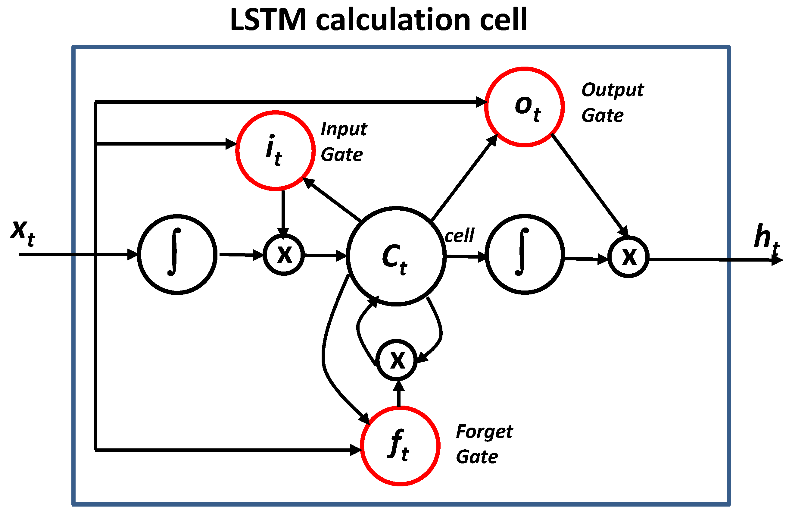
  • ‘We will use an LSTM (Long Short Term Memory) network. Recurrent networks take as input not only the example of current input they see, but also what they have previously perceived. The decision taken by a recurrent network at the time t-1 influences the decision it will reach a moment later in time t: the recurrent networks have two sources of input, the present and the recent past. We will use on each neuron the RELU activation function that flattens the response to all negative values to zero, while leaving everything unchanged for values equal to or greater than zero (normalization)’
  • model = Sequential()
  • model.add(LSTM(32, input_shape = (8,1), return_sequences = True, kernel_initializer = ‘uniform’, activation = ‘relu’))
  • model.add(LSTM(64, kernel_initializer = ‘uniform’, return_sequences = True, activation = ‘relu’ ))
  • model.add(LSTM(128, kernel_initializer = ‘uniform’, activation = ‘relu’))
  • model.add(Dense(256, activation = ‘relu’))
  • model.add(Dense(128, activation = ‘relu’))
  • model.add(Dense(64, activation = ‘relu’))
  • model.add(Dense(16, activation = ‘relu’))
  • model.add(Dense(1, activation = ‘sigmoid’))
  • ‘Loss function’
  • ‘We compile the model using as a NADAM optimizer that combines the peculiarities of the RMSProp optimizer with the momentum concept’
  • ‘We calculate the loss function through the binary crossentropy’
  • model.compile(loss = ‘binary_crossentropy’, optimizer = ‘NADAM’, metrics = [‘accuracy’])
  • model.summary()
  • # Fit the model
  • history = model.fit(X, Y, validation_split = 0.33, epochs = 300, batch_size = 64, verbose = 1)
  • ‘Graphical Reporting’
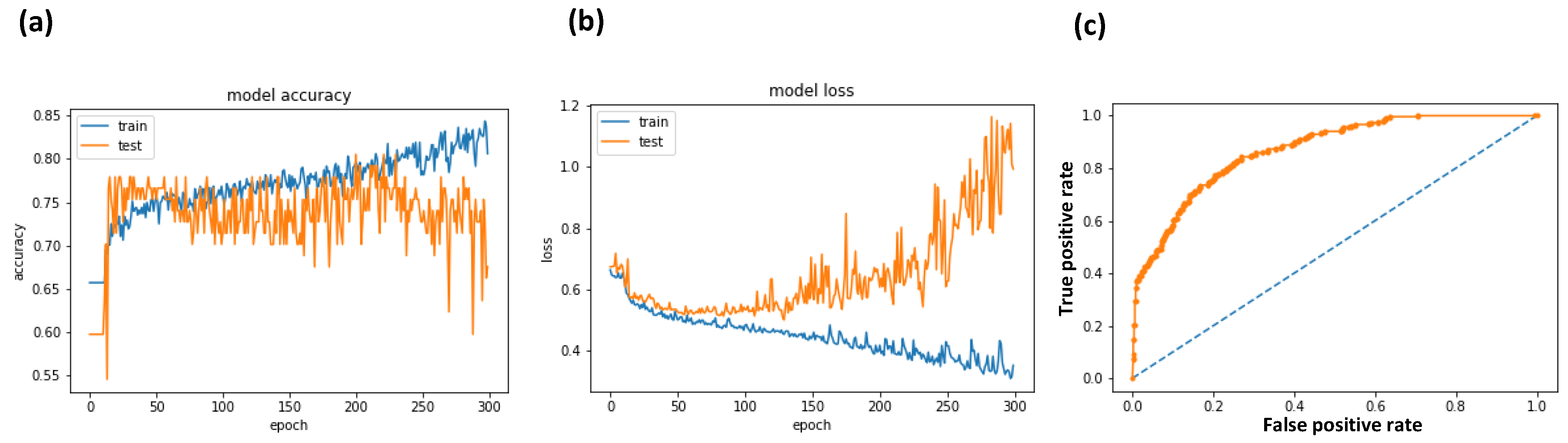
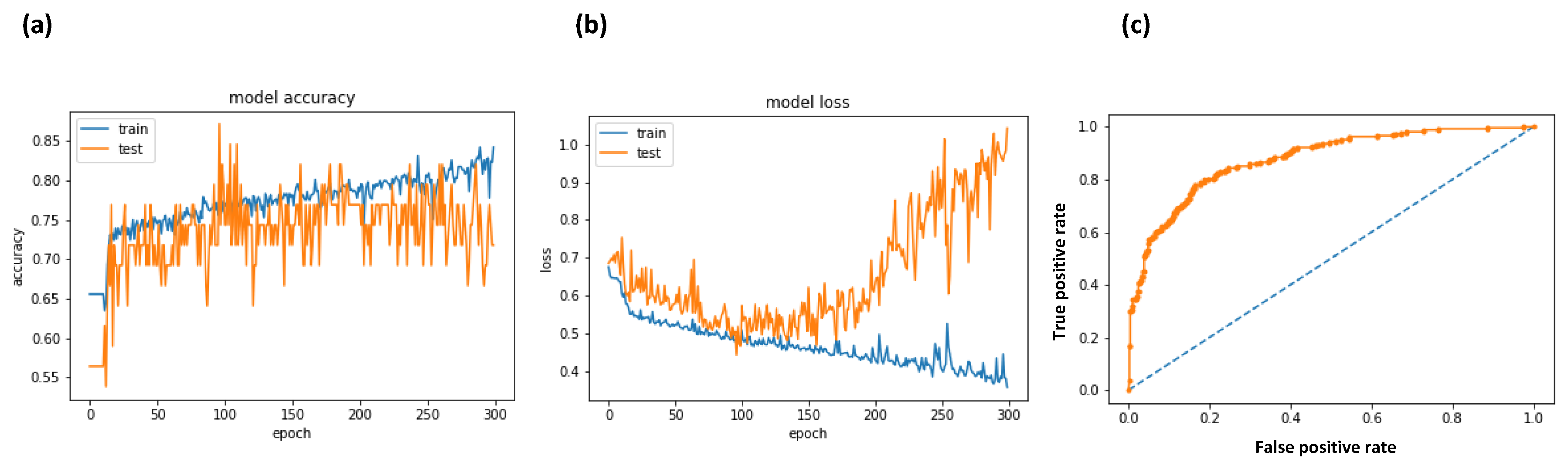
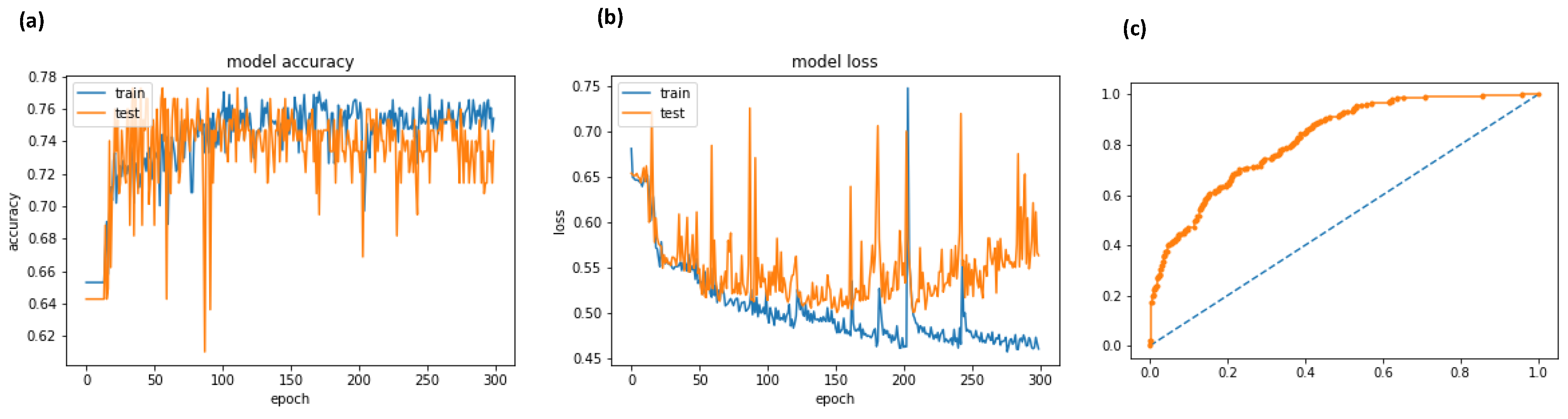
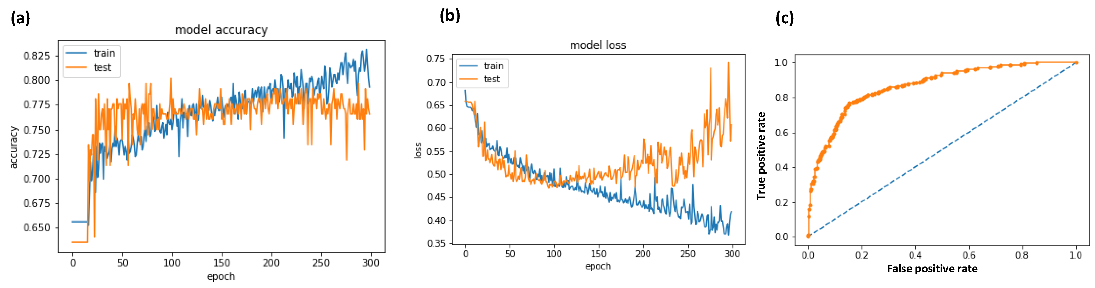
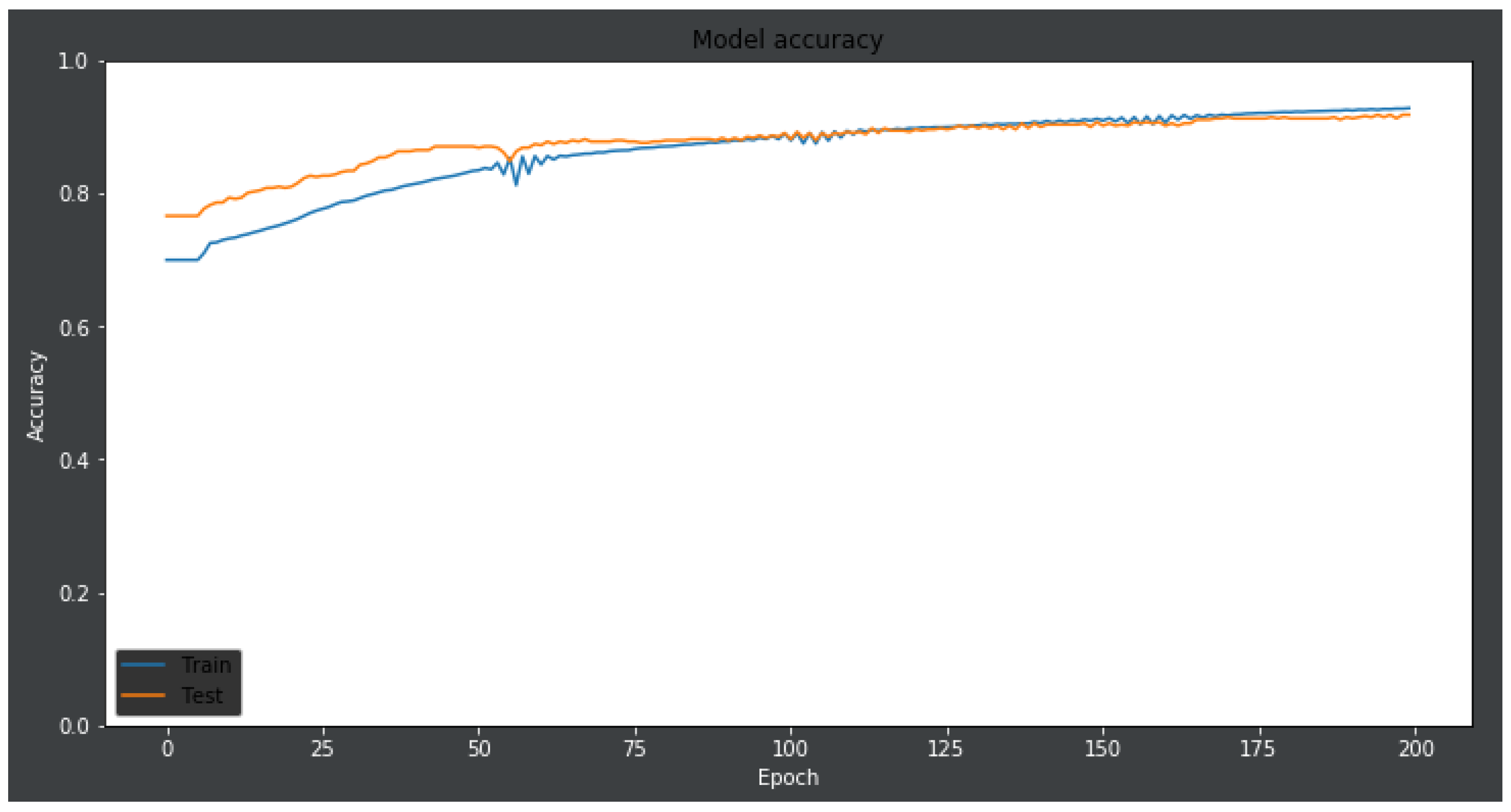
  • plt.plot(history.history[‘acc’])
  • plt.plot(history.history[‘val_acc’])
  • plt.title(‘model accuracy’)
  • plt.ylabel(‘accuracy’)
  • plt.xlabel(‘epoch’)
  • plt.legend([‘train’, ‘test’], loc = ‘upper left’)
  • plt.savefig(‘accuracy.png’)
  • plt.show()
  • ‘Outputs plotting’
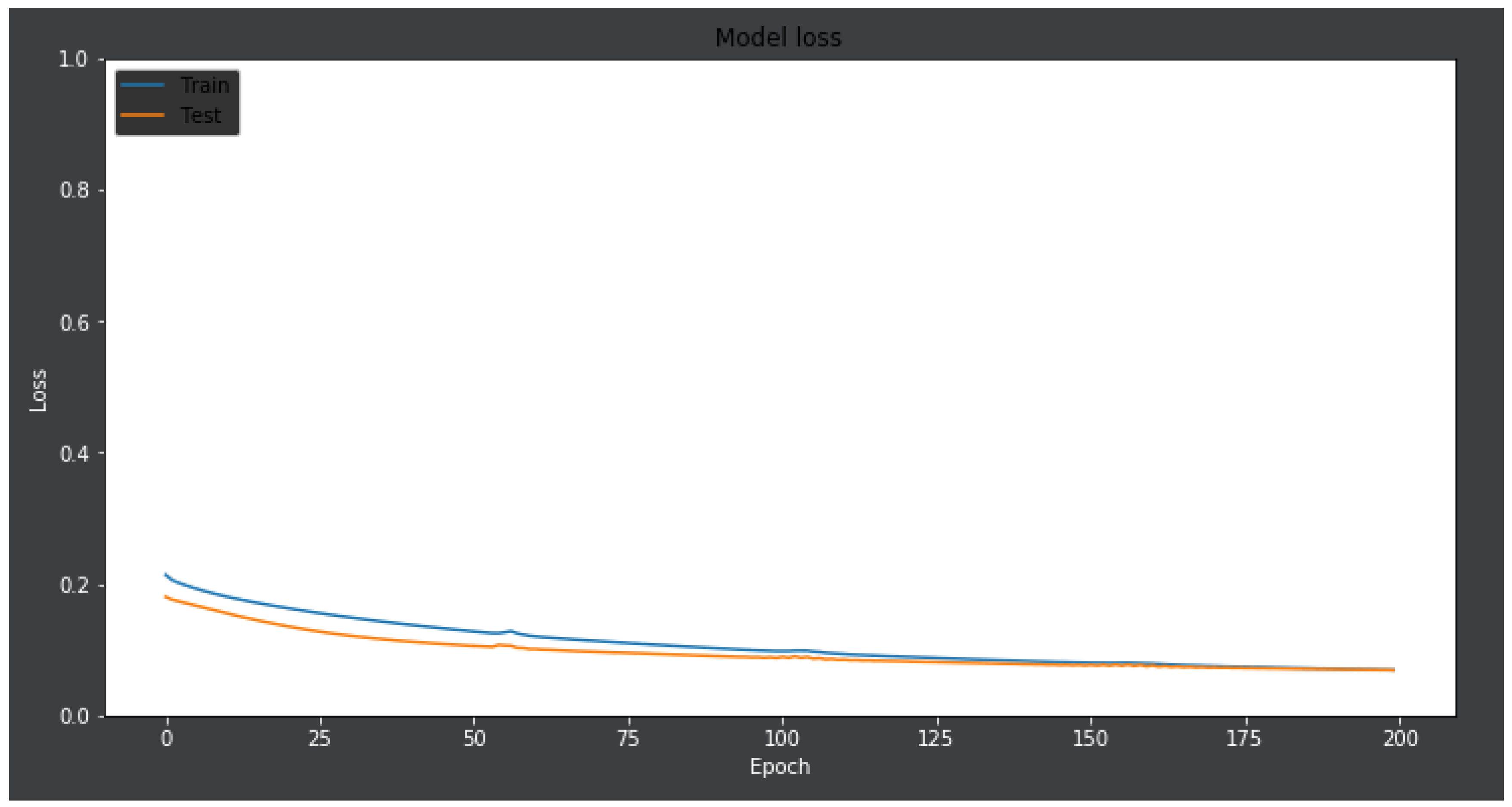
  • plt.plot(history.history[‘loss’])
  • plt.plot(history.history[‘val_loss’])
  • plt.title(‘model loss’)
  • plt.ylabel(‘loss’)
  • plt.xlabel(‘epoch’)
  • plt.legend([‘train’, ‘test’],loc = ‘upper left’)
  • plt.savefig(‘loss.png’)
  • plt.show()
  • ‘model saving’
  • model.save(‘pima_indian.model’)
  • ‘Curva ROC Curve’
  • probs = model.predict_proba(X)
  • probs = probs[:,0]
  • auc = roc_auc_score(Y, probs)
  • print(‘AUC: %.3f’ % auc)
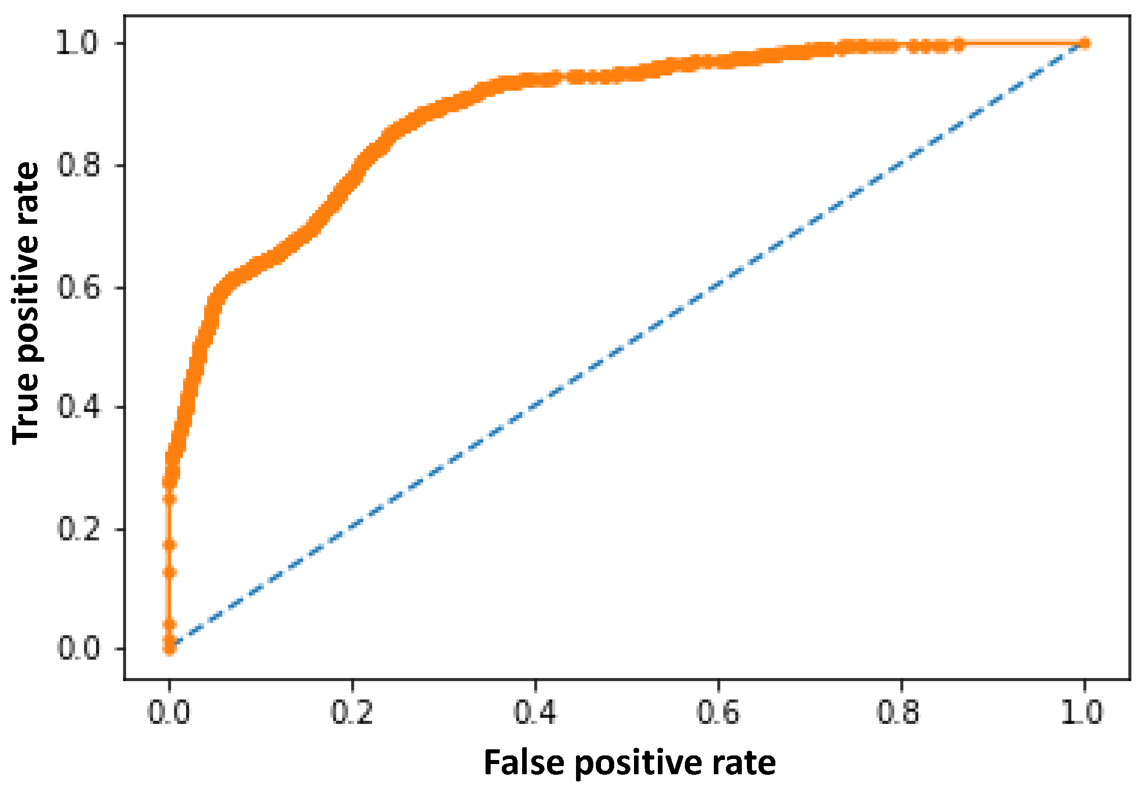
  • fpr, tpr, thresholds = roc_curve(Y, probs)
  • pyplot.plot([0, 1], [0, 1], linestyle = ‘--’)
  • pyplot.plot(fpr, tpr, marker = ‘.’)
  • pyplot.savefig(‘roc.png’)
  • pyplot.show()

Appendix B

In this appendix section is indicated the whole dataset structure of the information system monitoring patients at home. Figure A1 illustrates the database layout design upgrading the information system architecture of Figure 1a.
Figure A1. Database structure of the information system oriented on homecare assistance monitoring and integrating LSTM algorithms.
Applsci 09 03532 g0a1
Below are indicated the main requirements of the designed database enhancing possible facilities.
1. Model for alarm prediction
The patient ID, of sex SEX, having pathology pathology, born on BithDay, is examined at home by the id_devices providing measurements which will be stored in the database. The patient therapeutic status is indicated by id-therapia. Alarms is a tuple that contains the relative code_parameter and with the min and max values of the parameter that produced the alarm (thresholds).
2. Predictive model of patient’s health status
It is possible to predict the status of patients by applying the LSTM algorithm based on historical data processing of vital parameters dataset.
3. Classification of the adequacy of therapy for each patient who has experienced an alarm
All patient with id_parameters_threshold having a value above or below the threshold limit, are involved in a particular therapeutic status identified by id_therap_status, and by particular measures of pathology. Id_therap is the therapy that the patient is following. Every patient with a pathology follows a specific therapeutic program. If the patient’s state of health is recorded as critical, then, it will be possible to use an LSTM-based program which, based on historical data, will provide support about the adequacy of his therapy.
4. Support for the diagnosis and prognosis of the disease
Starting with the analysis of historical data, it is possible to establish the temporal evolution of the pathology. For example, it is possible to identify the patient that is most “similar” to the current patient. The patient id_patient is hospitalized on the first day by communicating messages to the operator, who receives documents typology (document_typology), containing filename (properly processed). The LSTM will provide a diagnostic indication of the pathology and a prognostic on its temporal evolution.
5. Evaluation of the human resources (operators)
The patient assistance operations will provide important information about Key Performance Indicators (KPI) of operators.
6. Documents data processing for the development of assisted diagnosis assistances
The data processing of all the documents and file about a patient will allow to optimize the homecare assistance process.
7. Analysis of the relationships between classes
Proper association rules allow us to obtain interesting relationships within the database attributes. In this case it is possible to establish relationships of the type: [id_patient, pathology] -> “parameters”, thus supporting the prognostic.
8. Analysis of devices
The device records will contain the identification number of the device associated with the patient. All data of devices will be contained into tables associated with the patient ID.
9. Inspection of the pharmacological dosage administered to the patient
At each patient id_patient is associated with a therapy id_therapy. An important relationship to analyze is: id_patient, id_therapy] -> “alarm”.
10. Real time Criticality analysis
The constantly monitored patient conditions can be displayed in real time. Historical measures can be applied in order to predict critical moments.

Appendix C

Below are listed the MLP script enabling data processing.
  • model = Sequential()
  • model.add(Dense(93, input_shape = (1200,), activation = ‘relu’))
  • model.add(Dense(93, activation = ‘relu’))
  • model.add(Dense(1, activation = ‘relu’))
  • model.compile(metrics = [‘accuracy’, auroc], optimizer = Nadam(lr = 0.002, schedule_decay = 0.004), loss = ‘mean_squared_error’)
  • model.summary()
Below are the reported model summary
Layer (type)Output Shape Param #
dense_1 (Dense)(None, 93) 111693
dense_2 (Dense)(None, 93)8742
dense_3 (Dense) (None, 1)94
Total params: 120,529
Trainable params: 120,529
Non-trainable params: 0

References

  1. Wimmer, H.; Powell, L.M. A comparison of open source tools for data science. J. Inf. Syst. Appl. Res. 2016, 9, 4–12. [Google Scholar]
  2. Al-Khoder, A.; Harmouch, H. Evaluating four of the most popular open source and free data mining tools. Int. J. Acad. Sci. Res. 2015, 3, 13–23. [Google Scholar]
  3. Gulli, A.; Pal, S. Deep Learning with Keras- Implement Neural Networks with Keras on Theano and TensorFlow; Birmingham- Mumbai Packt Book: Birmingham, UK, 2017; ISBN 978-1-78712-842-2. [Google Scholar]
  4. Kovalev, V.; Kalinovsky, A.; Kovalev, S. Deep learning with theano, torch, caffe, TensorFlow, and deeplearning4j: Which one is the best in speed and accuracy? In Proceedings of the XIII International Conference on Pattern Recognition and Information Processing, Minsk, Belarus, 3–5 October 2016; Belarus State University: Minsk, Belarus, 2016; pp. 99–103. [Google Scholar]
  5. Li, J.-S.; Yu, H.-Y.; Zhang, X.-G. Data mining in hospital information system. In New Fundamental Technologies in Data Mining; Funatsu, K., Ed.; Intech: London, UK, 2011. [Google Scholar]
  6. Goodwin, L.; VanDyne, M.; Lin, S. Data mining issues an opportunities for building nursing knowledge. J. Biomed. Inform. 2003, 36, 379–388. [Google Scholar] [CrossRef]
  7. Belacel, N.; Boulassel, M.R. Multicriteria fuzzy assignment method: A useful tool to assist medical diagnosis. Artif. Intell. Med. 2001, 21, 201–207. [Google Scholar] [CrossRef]
  8. Demšar, J.; Zupan, B.; Aoki, N.; Wall, M.J.; Granchi, T.H.; Beck, J.R. Feature mining and predictive model construction from severe trauma patient’s data. Int. J. Med. Inform. 2001, 36, 41–50. [Google Scholar] [CrossRef]
  9. Kusiak, A.; Dixon, B.; Shital, S. Predicting survival time for kidney dialysis patients: a data mining approach. Comput. Biol. Med. 2005, 35, 311–327. [Google Scholar] [CrossRef]
  10. Yu, H.-Y.; Li, J.-S. Data mining analysis of inpatient fees in hospital information system. In Proceedings of the IEEE International Symposium on IT in Medicine & Education (ITME2009), Jinan, China, 14–16 August 2009. [Google Scholar]
  11. Chae, Y.M.; Kim, H.S. Analysis of healthcare quality indicator using data mining and decision support system. Exp. Syst. Appl. 2003, 24, 167–172. [Google Scholar] [CrossRef]
  12. Morando, M.; Ponte, S.; Ferrara, E.; Dellepiane, S. Definition of motion and biophysical indicators for home-based rehabilitation through serious games. Information 2018, 9, 105. [Google Scholar] [CrossRef]
  13. Ozcan, Y.A. Quantitative Methods in Health Care Management, 2nd ed.; Josey-Bass: San Francisco, CA, USA, 2009; pp. 10–44. [Google Scholar]
  14. Ghavami, P.; Kapur, K. Artificial neural network-enabled prognostics for patient health management. In Proceedings of the IEEE Conference on Prognostics and Health Management (PHM), Denver, CO, USA, 18–21 June 2012. [Google Scholar]
  15. Grossi, E. Artificial neural networks and predictive medicine: A revolutionary paradigm shift. In Artificial Neural Networks—Methodological Advances and Biomedical Applications, 1st ed.; Suzuki, K., Ed.; InTech: Rijeka, Croatia, 2011; Volume 1, pp. 130–150. [Google Scholar]
  16. Adhikari, N.C.D. Prevention of heart problem using artificial intelligence. Int. J. Artif. Intell. Appl. 2018, 9, 21–35. [Google Scholar] [CrossRef]
  17. Galiano, A.; Massaro, A.; Boussahel, B.; Barbuzzi, D.; Tarulli, F.; Pellicani, L.; Renna, L.; Guarini, A.; De Tullio, G.; Nardelli, G.; et al. Improvements in haematology for home health assistance and monitoring by a web based communication system. In Proceedings of the IEEE International Symposium on Medical Measurements and Applications MeMeA, Benevento, Italy, 15–18 May 2016. [Google Scholar]
  18. Massaro, A.; Maritati, V.; Savino, N.; Galiano, A.; Convertini, D.; De Fonte, E.; Di Muro, M. A Study of a health resources management platform integrating neural networks and DSS telemedicine for homecare assistance. Information 2018, 9, 176. [Google Scholar] [CrossRef]
  19. Massaro, A.; Maritati, V.; Savino, N.; Galiano, A. Neural networks for automated smart health platforms oriented on heart predictive diagnostic big data systems. In Proceedings of the AEIT 2018 International Annual Conference, Bari, Italy, 3–5 October 2018. [Google Scholar]
  20. Saadatnejad, S.; Oveisi, M.; Hashemi, M. LSTM-based ECG classification for continuous monitoring on personal wearable devices. IEEE J. Biomed. Health Inform. 2019. [Google Scholar] [CrossRef] [PubMed]
  21. Pham, T.; Tran, T.; Phung, D.; Venkatesh, S. Predicting healthcare trajectories from medical records: A deep learning approach. J. Biomed. Inform. 2017, 69, 218–229. [Google Scholar] [CrossRef] [PubMed]
  22. Kaji, D.A.; Zech, J.R.; Kim, J.S.; Cho, S.K.; Dangayach, N.S.; Costa, A.B.; Oermann, E.K. An attention based deep learning model of clinical events in the intensive care unit. PLoS ONE 2019, 14, e0211057. [Google Scholar] [CrossRef] [PubMed]
  23. Pima Indians Diabetes Database. Available online: https://gist.github.com/ktisha/c21e73a1bd1700294ef790c56c8aec1f (accessed on 27 August 2019).
  24. Predict the Onset of Diabetes Based on Diagnostic Measures. Available online: https://www.kaggle.com/uciml/pima-indians-diabetes-database (accessed on 21 June 2019).
  25. Wu, H.; Yang, S.; Huang, Z.; He, J.; Wang, X. Type 2 diabetes mellitus prediction model based on data mining. Inform. Med. Unlocked 2018, 10, 100–107. [Google Scholar] [CrossRef]
  26. Luo, M.; Ke Wang, M.; Cai, Z.; Liu, A.; Li, Y.; Cheang, C.F. Using imbalanced triangle synthetic data for machine learning anomaly detection. Comput. Mater. Contin. 2019, 58, 15–26. [Google Scholar] [CrossRef]
  27. Al Helal, M.; Chowdhury, A.I.; Islam, A.; Ahmed, E.; Mahmud, S.; Hossain, S. An optimization approach to improve classification performance in cancer and diabetes prediction. In Proceedings of the International Conference on Electrical, Computer and Communication Engineering (ECCE), Cox’sBazar, Bangladesh, 7–9 February 2019. [Google Scholar]
  28. Li, T.; Fong, S. A fast feature selection method based on coefficient of variation for diabetics prediction using machine learning. Int. J. Extr. Autom. Connect. Health 2019, 1, 1–11. [Google Scholar] [CrossRef]
  29. Puneet, M.; Singh, Y.A. Impact of preprocessing methods on healthcare predictions. In Proceedings of the 2nd International Conference on Advanced Computing and Software Engineering (ICACSE), Sultanpur, India, 8–9 February 2019. [Google Scholar]
  30. Stranieri, A.; Yatsko, A.; Jelinek, H.F.; Venkatraman, S. Data-analytically derived flexi, le HbA1c thresholds for type 2 diabetes mellitus diagnostic. Artif. Intell. Res. 2016, 5, 111–134. [Google Scholar]
  31. Sudharsan, B.; Peeples, M.M.; Shomali, M.E. Hypoglycemia prediction using machine learning models for patients with type 2 diabetes. J. Diabetes Sci. Technol. 2015, 9, 86–90. [Google Scholar] [CrossRef]
  32. Mhaskar, H.N.; Pereverzyev, S.V.; Van Der Walt, M.D. A deep learning approach to diabetic blood glucose prediction. Front. Appl. Math. Stat. 2017, 3, 1–14. [Google Scholar] [CrossRef]
  33. Contreras, I.; Vehi, J. Artificial intelligence for diabetes management and decision support: Literature review. J. Med. Internet Res. 2018, 20, 1–24. [Google Scholar] [CrossRef]
  34. Bosnyak, Z.; Zhou, F.L.; Jimenez, J.; Berria, R. Predictive modeling of hypoglycemia risk with basal insulin use in type 2 diabetes: Use of machine learning in the LIGHTNING study. Diabetes Ther. 2019, 10, 605–615. [Google Scholar] [CrossRef] [PubMed]
  35. Massaro, A.; Meuli, G.; Galiano, A. Intelligent electrical multi outlets controlled and activated by a data mining engine oriented to building electrical management. Int. J. Soft Comput. Artif. Intell. Appl. 2018, 7, 1–20. [Google Scholar] [CrossRef]
  36. Myers, J.L.; Well, A.D. Research Design and Statistical Analysis, 2nd ed.; Lawrence Erlbaum: Mahwah, NJ, USA, 2003. [Google Scholar]
  37. Hochreiter, S.; Schmidhuber, J. Long short-term memory. Neural Comput. 1997, 9, 1735–1780. [Google Scholar] [CrossRef] [PubMed]
  38. Mohapatra, S.K.; Mihir, J.K.S.; Mohanty, N. Detection of diabetes using multilayer perceptron. In International Conference on Intelligent Computingand Applications, Advances in Intelligent Systems and Computing; Bhaskar, M.A., Dash, S.S., Das, S., Panigrahi, B.K., Eds.; Springer: Singapore, 2019. [Google Scholar]
  39. Swets, J.A. Measuring the accuracy of diagnostic systems. Science 1988, 240, 1285–1293. [Google Scholar] [CrossRef] [PubMed]
  40. Diabetes Data Set. Available online: https://archive.ics.uci.edu/ml/datasets/Diabetes (accessed on 19 August 2019).
  41. Chui, K.T.; Fung, D.C.L.; Lytras, M.D. Predicting at-risk University students in a virtual learning environment via a machine learning algorithm. Comput. Hum. Behav. 2018, in press. [Google Scholar] [CrossRef]
Figure 1. (a) Architecture of homecare smart assistance platform based on artificial neural networks (ANN) data processing [19]; (b) Konstanz Information Miner (KNIME) workflow implementing a traditional ANN multi-layer perceptron (MLP) [19].
Applsci 09 03532 g001
Figure 2. (ai) Attribute dataset statistic distribution.
Applsci 09 03532 g002
Figure 3. Outcome versus DiabetesPedigree function.
Applsci 09 03532 g003
Figure 4. Outcome versus Insulin function.
Applsci 09 03532 g004
Figure 5. Outcome versus BMI function.
Applsci 09 03532 g005
Figure 6. Long short-term memory (LSTM) calculation cell (symbol x represents the multiplication operator between inputs, and ∫ represents the application of a differentiable function).
Applsci 09 03532 g006
Figure 7. LSTM results (training dataset = 95%, testing dataset = 5%): (a) Model accuracy versus epochs; (b) model loss versus epochs; (c) receiver operating characteristics (ROC) curve.
Applsci 09 03532 g007
Figure 8. LSTM results (training dataset = 90%, testing dataset = 10%): (a) Model accuracy versus epochs; (b) model loss versus epochs; (c) ROC curve.
Applsci 09 03532 g008
Figure 9. LSTM results (training dataset = 85%, testing dataset = 15%): (a) Model accuracy versus epochs; (b) model loss versus epochs; (c) ROC curve.
Applsci 09 03532 g009
Figure 10. LSTM results (training dataset = 80%, testing dataset = 20%): (a) Model accuracy versus epochs; (b) model loss versus epochs; (c) ROC curve.
Applsci 09 03532 g010
Figure 11. LSTM results (training dataset = 75%, testing dataset = 25%): (a) Model accuracy versus epochs; (b) model loss versus epochs; (c) ROC curve.
Applsci 09 03532 g011
Figure 12. LSTM-AR- results (training dataset = 80%, testing dataset = 20%): Model Accuracy versus epochs.
Applsci 09 03532 g012
Figure 13. LSTM-AR- results (training dataset = 80%, testing dataset = 20%): Model Loss versus epochs.
Applsci 09 03532 g013
Figure 14. LSTM-AR- results (training dataset = 80%, testing dataset = 20%): ROC curve.
Applsci 09 03532 g014
Figure 15. Flowchart representing automatisms for LSTM/LSTM-AR- DSS model predicting diabetes.
Applsci 09 03532 g015
Figure 16. Accuracy plot using dataset found in reference [40].
Applsci 09 03532 g016
Figure 17. Loss plot using dataset found in reference [40].
Applsci 09 03532 g017
Table 1. Correlation matrix between experimental dataset attributes.
PNGPBPDSTTIBMIDPFDAAOC
PN10.130.14−0.08−0.070.02−0.030.540.22
GP0.1310.150.060.030.220.140.260.47
BPD0.140.1510.210.090.280.040.240.07
STT−0.080.060.2110.040.390.18−0.110.07
I−0.070.330.090.4410.20.19−0.040.13
BMI0.020.220.280.390.0210.140.040.29
DPFD−0.030.140.040.180.190.1410.030.17
AA0.540.260.24−0.11−0.040.040.0310.24
OC0.220.470.070.070.10.290.170.241
Table 2. Example of predicted outcomes (diabetes prediction): OC is the labeled class.
PNGPBPDSTTIBMIDPFDAAOC (Predicted)
61487235033.60.627501
1856629026.60.351310
8183640023.30.672321
18966239428.10.167210
0137403516843.12.288331
5116740025.60.201300
37850328831.00.248261
1011500035.30.134290
2197704554330.50.158531
8125960000.232541
Table 3. LSTM neural network model and decision support systems (DSS) reading automatism: area under the curve (AUC), accuracy, and loss results.
Testing Samples 5%10%15%20%25%
AUC %87.78783.98286.7
Accuracy %7573707576
Loss %100100705565
Table 4. Cross validation of results.
MethodTest Set Accuracy %
MLP77.5 [38]
LSTM75
LSTM-AR-84
Table 5. LSTM/LSTM-AR models and DSS reading automatism: AUC, accuracy and loss results.
Testing Samples LSTM (20%) LSTM-AR (20%)
AUC %8289
Accuracy %7584
Loss %5550
For the other testing dataset (5%, 10%, 15%, 25%) the same increase/decrease percentage has been observed as in the case of Table 5.
Table 6. AUC values [39].
AUCAUC < 0.5 (50%)AUC = 0.50.5 (50%) < AUC ≤ 0.7 (70%)0.7 (70%) < AUC ≤ 0.9 (90%)0.9 (90%) < AUC ≤ 1 (100%)AUC = 1
Classification of the discriminating capacity of a testNo sense testNon-informative testInaccurate testModerately accurate testHighly accurate testPerfect test
Table 7. Limitations and advantages of the proposed study.
AdvantagesLimitations
DSS tool for diabetes prediction ready to useAccurate training dataset
Multi attribute analysisRedundancy of data processing (correlated attributes)
Reading procedure of outputs resultsPresence of positive false and negative false due to wrong measurements
Choose of the best model according to simultaneous analyses (accuracy, loss, and AUC)Finding a true compromise of efficiency parameter values
Network having a memory used for the data processingIt is necessary to acquire a correct temporal data sequence
Powerful approach if compared with ANN MLP methodHigh computational cost
Table 8. LSTM, LSTM-AR, and MLP models: AUC, accuracy and loss results by considering the dataset found in reference [40].
Testing Samples LSTM (20%) LSTM-AR (20%)MLP (20%)
AUC %919194
Accuracy %868682
Loss %10 1014

