On the Determination of Meshed Distribution Networks Operational Points after Reinforcement

Abstract

This paper proposes a calculation algorithm that creates operational points and evaluates the performance of distribution lines after reinforcement. The operational points of the line are probabilistically determined using Monte Carlo simulation for several objective functions for a given line. It is assumed that minimum voltage at all nodes has to be balanced to the maximum load served under variable distributed generation production, and to the energy produced from the intermittent renewables. The calculated maximum load, which is higher than the current load, is expected to cover the expected needs for electric vehicles charging. Following the proposed operational patterns, it is possible to have always maximum line capacity. This method is able to offer several benefits. It facilitates of network planning and the estimation of network robustness. It can be used as a tool for network planners, operators and large users. It applies to any type of network including radial and meshed.

1. Introduction

Medium and low voltage distribution networks are mostly operated as radial; however, in some exceptional cases, they can be connected as meshed or in loops [1]. Radial circuits have many advantages over networked circuits, including easier fault current protection, lower fault currents over most of the circuit, easier voltage control, easier prediction and control of power flows and lower installation cost [2]. On the other hand, meshed networks demonstrate performance improvements and efficiency increase. The reinforcement of already existing distribution networks is an issue of priority for network operators, in an effort to ensure the uninterruptable power supply. Several works have been developed to investigate reinforcement issues in radial and meshed distribution level and to provide adequate simulation tools and methods. Alvarez-Herault et al. [3] demonstrated the benefits of meshing the network instead of reinforcing it. Novoselnik et al. [4] provided a procedure to improve networks’ performance taking into consideration the advantage of its meshed development. The networks operate in radial mode even if they are built as meshed. This article proposes a control method to optimally rearrange the radial network. Nevertheless, in this case the network continues to operate radially. Moreover, several planning methods take into consideration that optimal solutions can lead to meshed networks [5], even if they are weakly meshed. Recently, optimization for distribution network planning has led to substantial research activity even if part of the researcher community still supports, to a certain degree, the benefits of distribution system radial operation [6].

Added to the above, the increasing use of electric vehicles and the consequent impact on the operation of the network has to be taken into consideration. Note that the penetration level of electric vehicles is higher in the countries where the appropriate infrastructure is widely available [7]. Hence, their charging and their interaction in general with the electricity network can be controlled remotely in a safe manner, maybe by a charging service provider (CSP) [8,9] or on individual vehicle basis [10]. Given the already major resources provided to build the infrastructure, their charging can be prioritized on grid requirements. This would on one hand meet possible infrastructure constraints and on the other hand improve electricity system performance, even though new significant load is added. Furthermore, this procedure would offer time for system reinforcements, if these are needed.

However, system inertia exists in the system, and hence, controlled charging has to be achieved gradually [11]. It can start from lower penetration of electric vehicles and random charging when needed, up to the level where electric vehicles would charge only when grid has the essential capacity to allocate in this exercise. In this way, electric vehicles are behaving as battery storage [12]. The proposed procedure would also be enhanced in the future from improved battery performance connected to enhanced electric vehicle range that would reduce driver anxiety. However, in any case, this approach could decrease vehicle owners’ satisfaction who are used to a continued service currently offered from fossil fuel powered vehicles. This approach could also possibly deteriorate battery condition. Of course, on the other hand, drivers’ behavior affects, in a different manner, electricity systems [13].

Additionally, it could create discomfort to the industry [14] that is going to implement the incentive, but the benefits are more important to the effort. It has to be mentioned that electricity companies already have the experience in operating demand side management programs, restricted by the limited communication resources of the past. These demand side management programs are not considered as suitable for electric vehicles optimal charging [15]. Building upon this direction, bibliography proposes electric vehicle charging regulation that is organized on the transmission system or to the level of the distribution network based on a range of decision factors [16] that have to do with operational conditions or production from intermitted renewables.

Having mentioned the above, electric vehicles are to be charged in a way to provide always the necessary load [17]. This approach would contribute in achieving grid operational optimization as it is also projected in this study. This optimization would be based on the incoming intermittent energy from renewables connected to the distribution grid and the voltage profile of the line under investigation.

Except from the electric vehicles, the already widely developed connection of distributed generation [18] affects the operation of the grid. It creates bidirectional power flows [19] and changes network topology. As expected, network planning with distributed generation research applies similar to meshed network planning optimization methods [20,21]. Meshed planning in conjunction to the connection of distributed generation could potentially enhance network’s operation [22]. It has to be mentioned that in our work all components are assumed as functioning; however, in practice there could be malicious and faulty units [23].

Several optimization methods are being used for distribution network analysis, including Tabu search (TS), Simulated annealing (SA), Genetic algorithm (GA), Evolutionary strategy (ES), Artificial immune system (AIS), Ant colony optimization (ACO), Ant colony system (ACS), Particle swarm optimization (PSO) and Hybrid TS/GA (Memetic) [24]. This research is based on the Monte Carlo method [25], which is implemented to a plethora of applications [26], including network planning. On power systems, it is widely used to simulate probabilistic phenomena [27] in general, and power flows for steady state simulations [28]. Active distribution [29] and expansion [30] planning under uncertainty remains an issue of paramount importance. The dynamic programming method is a viable alternative [31]. Monte Carlo is frequently the method of choice to this direction [32]. It requires, even for today’s standards, high computational power; hence, for the simulations of this work, Okeanos cloud computing [33] is used, which is a supercomputing facility, organized on virtual machines available to the research community.

All the proposed methods for distribution network planning seek to optimize a value directly related to grids’ operation. This could be total installation and operational cost, minimum power or copper losses or voltage deviation. The proposed solutions up to today offer a deterministic approach towards solving the given electric vehicle connection capacity problem. However, they lack the capability to enhance user’s decision making capability offering additional information of system robustness, behavior and performance after reinforcement. This could be a useful tool for engineers who engage in network planning, operation and large users of the system. In this paper, a calculation procedure is developed in an effort to upgrade the operation of distribution grids, providing benefits in terms of their optimal point of operation that can be used for demand management purposes. It can be complimentary to any other optimization method for distribution grid planning. Moreover, it aims to demonstrate that distribution medium voltage network is better if operated as meshed and to provide solutions in terms of network planning. Its main contribution is the application of a novel method, based on Monte Carlo and objective functions to evaluate decisions for network reinforcement. This research is organized in three sections. Section 2. ‘System under examination and problem formulation’ describes the network under investigation and the procedure that it was followed to tackle the research question. Section 3, ‘Results and Discussion’ provides the outcome of our analysis and its commenting. Section 4 contains the conclusions and future work.

2. System under Examination and Problem Formulation

Table 1. Network topology.

Line (Node→Node)	Length [km]	Cross Section [mm2]	Line (Node→Node)	Length [km]	Cross Section [mm2]
1→2	0.25	95	57→58	0.483	35
1→3	2.305	95	58→59	0.677	35
2→4	0.488	95	58→60	0.014	16
4→5	0.945	35	61→62	0.5	95
6→4	0.505	95	61→63	0.1	95
6→7	0.333	95	64→63	0.648	16
6→8	0.132	16	65→63	0.1	95
7→9	0.473	16	65→66	0.18	16
7→10	1	95	66→67	0.524	16
10→11	0.55	95	66→68	0.169	16
11→12	0.179	95	68→117	0.22	16
11→13	0.068	35	68→69	0.014	16
11→14	0.242	95	70→71	0.507	16
14→15	0.521	95	70→72	0.008	35
14→16	0.363	16	73→74	0.01	35
15→17	0.6	95	75→76	0.01	35
17→18	0.225	16	75→77	0.01	35
17→19	0.197	95	78→79	0.451	35
19→20	0.208	95	78→80	0.043	35
20→21	0.008	35	80→81	0.479	35
20→22	0.006	95	82→83	0.571	35
22→23	0.334	95	82→81	0.01	35
22→24	0.785	35	84→85	1.384	35
25→26	2.419	35	84→86	0.022	35
26→27	3.125	35	87→88	0.075	35
26→28	0.258	35	89→84	0.244	35
29→30	0.871	16	90→82	0.266	16
30→31	0.14	16	90→91	0.4	16
32→33	0.304	95	90→92	0.06	16
32→34	0.311	16	93→94	4.968	16
32→35	0.108	95	95→93	0.6	16
35→36	0.469	35	96→95	0.228	16
36→37	0.465	35	92→97	0.359	16
36→38	0.661	95	97→98	0.007	16
38→39	0.5	35	99→97	0.368	16
38→40	0.447	95	100→101	0.018	16
41→40	0.326	16	102→3	0.001	95
42→43	0.082	95	103→104	0.07	35
42→44	0.3	16	105→104	0.198	35
42→40	0.343	95	106→49	0.001	35
45→46	1.365	16	107→83	0.006	35
45→47	0.023	35	108→98	0.01	35
48→45	1.275	16	109→78	0.487	35
46→49	0.102	35	110→28	0.14	35
46→50	10.181	16	111→37	0.298	35
51→52	0.777	35	112→37	0.001	35
52→53	0.286	35	113→80	0.125	35
52→54	0.702	35	114→35	0.277	35
54→55	0.076	35	115→81	0.356	35
54→56	0.414	35	116→87	1.297	35

,

Table 2. Installed capacity (S), maximum and minimum active and reactive loads (P_max, Q_max, P_min, Q_min) of each 20/0.4kV distribution transformer.

Node	S [kVA]	Pmax [kW]	Qmax [kVAr]	Pmin [kW]	Qmin [kVAr]	Node	S [kVA]	Pmax [kW]	Qmax [kVAr]	Pmin [kW]	Qmin [kVAr]
1	50	17	10	1	1	46	200	68	42	5	3
2	485	164	102	12	7	49	100	34	21	2	1
4	720	243	151	17	11	57	210	71	44	5	3
6	100	34	21	2	1	59	50	17	10	1	1
7	320	108	67	8	5	60	100	34	21	2	1
10	920	311	193	22	14	61	75	25	16	2	1
14	150	51	31	4	2	64	560	189	117	14	8
15	660	223	138	16	10	66	250	85	52	6	4
19	75	25	16	2	1	117	410	139	86	10	6
20	100	34	21	2	1	69	250	85	52	6	4
22	250	85	52	6	4	67	175	59	37	4	3
25	1490	504	312	36	22	12	160	54	34	4	2
26	100	34	21	2	1	16	100	34	21	2	1
28	50	17	10	1	1	71	160	54	34	4	2
27	360	122	75	9	5	73	160	54	34	4	2
29	810	274	170	20	12	75	250	85	52	6	4
31	100	34	21	2	1	96	160	54	34	4	2
9	410	139	86	10	6	94	250	85	52	6	4
34	100	34	21	2	1	92	100	34	21	2	1
40	100	34	21	2	1	98	160	54	34	4	2
41	160	54	34	4	2	99	160	54	34	4	2
45	50	17	10	1	1	101	50	17	10	1	1
50	545	184	114	13	8

and

Table 3. Renewable energy sources at every node.

Node	Installed Power [kW]	Node	Installed Power [kW]	Node	Installed Power [kW]
110	100	114	100	109	100
72	100	111	100	113	500
74	100	112	100	115	20
76	100	39	100	107	100
21	500	106	100	86	100
13	100	47	100	88	1274
103	100	55	470	116	1815
105	100	56	700	108	50

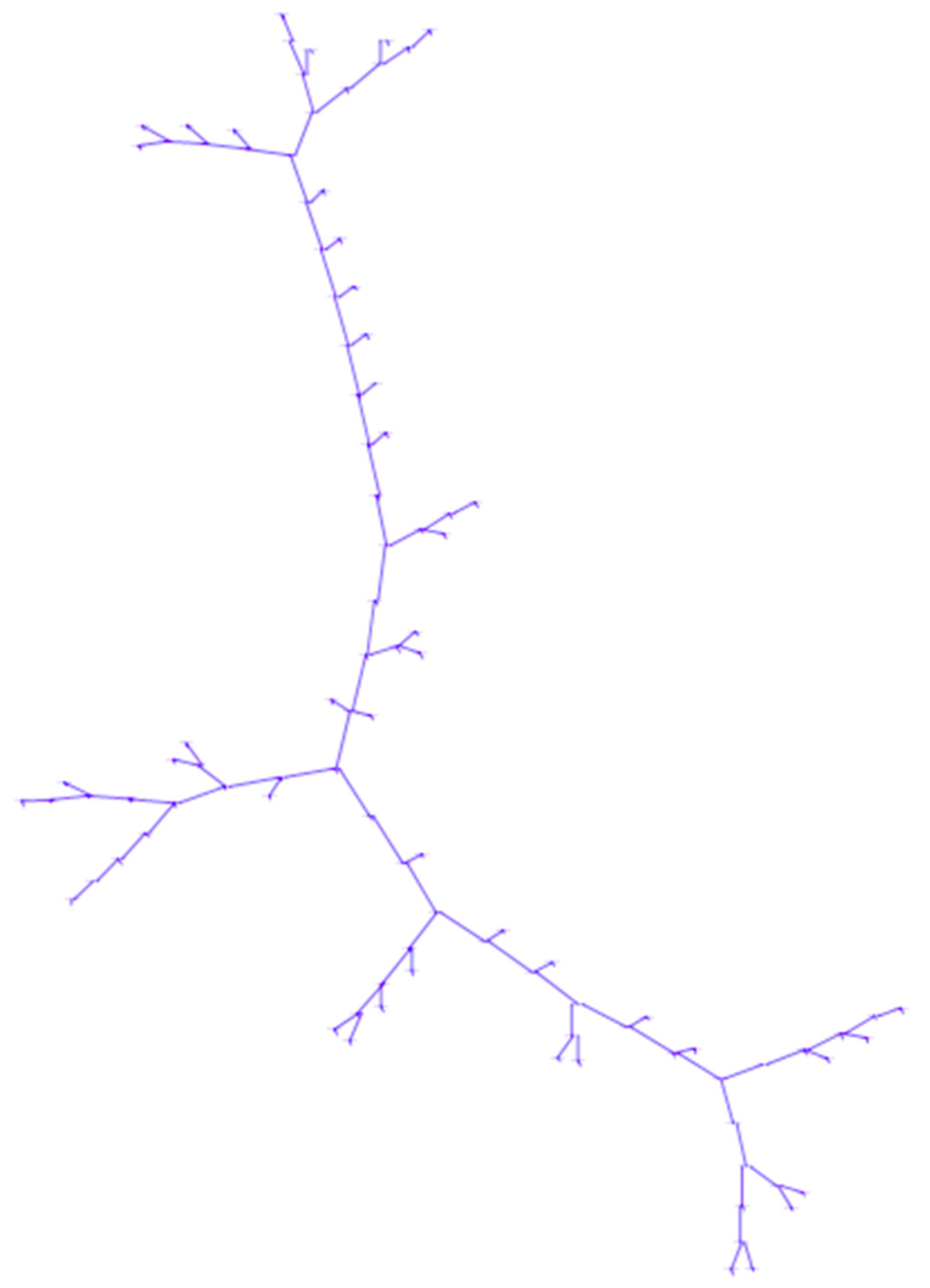
present the technical characteristics and the configuration of the distribution network under study [34]. An abstract graphical representation of the network is provided at Figure 1. The voltage level of the grid is 20 kV, the total length is 55 km and the installed capacity is 12 MVA. The network includes 45 20/0.4 kV distribution transformers and 24 renewable energy sources plants (photovoltaics). The resistance and the reactance of the conductors is R = 1.268 Ω/km and X = 0.422 Ω/km for ACSR 16 mm², R = 1.071 Ω/km and X = 0.393 Ω/km for ACSR 35 mm² and R = 0.215 Ω/km and X = 0.334 Ω/km for ACSR 95 mm². In order to improve the performance of this line [34] and to demonstrate the capability of the proposed method suitable for meshed networks, it is being reinforced in a meshed manner, connecting the nodes 51 and 84 using ACSR 95 mm² conductors. The distance between these nodes is 8 km, creating a resistance of 1.72 Ω and impedance of 2.672 Ω, or pu resistance and impedance 0.43 pu and 0.668 pu, respectively.

The total load of the line is the sum of all 20/0.4 kV transformers load and the production of renewables is fed to the line through the renewable energy sources connection points. Renewable energy sources connected to this line are located in the relatively proximity with each other. This is to the comparably limited size of a distribution line such as the one under investigation. Plants’ production is considered as analogous to their installed power but the same at each time period across all of the line since solar irradiation can be safely considered as being identical.

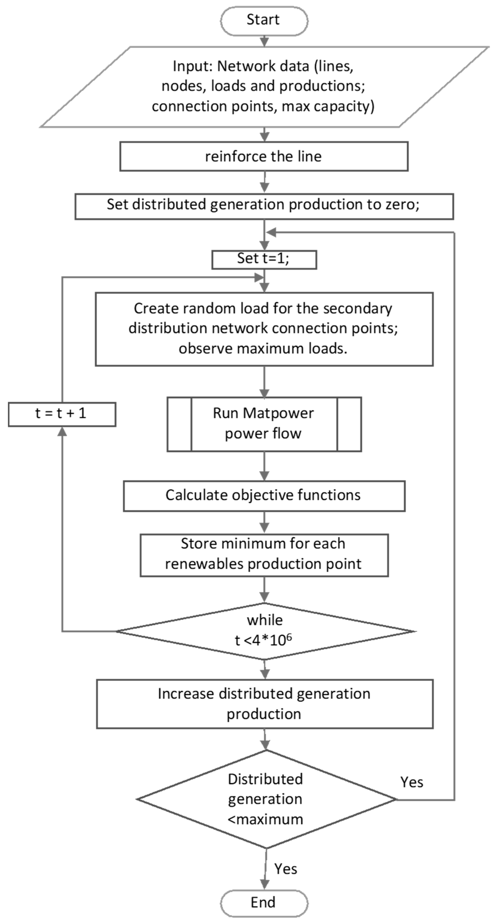
Figure 2 depicts the flow chart of the developed calculation procedure. The algorithm creates randomly possible loading for all transformers feeding the low voltage part of the distribution network and perform power flow analysis. Then, the values of the objective functions are calculated, and this algorithm reiterates 4 million times. The above procedure is being repeated for distributed generators production from 0 to full of their installed capacity in 1/10 steps of the maximum value.

AC power flow is used to perform the calculations for this analysis [35], by using an appropriate computer tool [25,26]. All nodes are PQ, being able to offer active and reactive power, except from the slack node. In this case, there is no generator connected. The distributed generators are simulated as negative loads given that based on research questions, their production is known. The following equations used to simulate the branches [36]:

$$\left[\frac{{\mathrm{i}}_{\mathrm{f}}}{{\mathrm{i}}_{\mathrm{t}}}\right]={\mathrm{Y}}_{\mathrm{br}}\left[\frac{{\mathrm{v}}_{\mathrm{f}}}{{\mathrm{v}}_{\mathrm{t}}}\right]$$

(1)

where: v_f, v_t, i_f and i_t are the terminal voltages and currents.

Equation (1) connects voltages at all nodes and currents. The impedance matrix (Y_br) expresses the impedances across all branches forming a table that is unique for each network.

The admittance matrix Y_br is as follows:

$${\mathrm{Y}}_{\mathrm{br}}=\left[\begin{array}{cc}{\mathrm{y}}_{\mathrm{ff}}^{\mathrm{i}}& {\mathrm{y}}_{\mathrm{ft}}^{\mathrm{i}}\\ {\mathrm{y}}_{\mathrm{tf}}^{\mathrm{i}}& {\mathrm{y}}_{\mathrm{tt}}^{\mathrm{i}}\end{array}\right]$$

(2)

Eventually, the balance equation based on Kirchhoff’s laws can be written as follows [35], f(V, Sg) needs to equal to zero:

$$\mathrm{f}\left(\mathrm{V},{\mathrm{S}}_{\mathrm{g}}\right)={\mathrm{S}}_{\mathrm{bus}}\left(\mathrm{V}\right)+{\mathrm{S}}_{\mathrm{d}}-{\mathrm{C}}_{\mathrm{g}}·{\mathrm{S}}_{\mathrm{g}}$$

(3)

where S_g, and S_d are the generators’ and loads’ apparent power, then (3) becomes [35] f_p(Θ, V_m, P_g) and fq(Θ, V_m, P_g) that also need to equal to zero:

$${\mathrm{f}}_{\mathrm{P}}\left(\mathsf{\Theta },{\mathrm{V}}_{\mathrm{m}},{\mathrm{P}}_{\mathrm{g}}\right)={\mathrm{P}}_{\mathrm{bus}}\left(\mathsf{\Theta },{\mathrm{V}}_{\mathrm{m}}\right)+{\mathrm{P}}_{\mathrm{d}}-{\mathrm{C}}_{\mathrm{g}}·{\mathrm{S}}_{\mathrm{g}}$$

(4)

$${\mathrm{f}}_{\mathrm{P}}\left(\mathsf{\Theta },{\mathrm{V}}_{\mathrm{m}},{\mathrm{P}}_{\mathrm{g}}\right)={\mathrm{Q}}_{\mathrm{bus}}\left(\mathsf{\Theta },{\mathrm{V}}_{\mathrm{m}}\right)+{\mathrm{Q}}_{\mathrm{d}}-{\mathrm{C}}_{\mathrm{g}}·{\mathrm{Q}}_{\mathrm{g}}$$

(5)

and:

$$\mathrm{g}\left(\mathrm{x}\right)=\left[\begin{array}{c}{\mathrm{f}}_{\mathrm{P}}^{\left\{\mathrm{i}\right\}}\left(\mathsf{\Theta },{\mathrm{V}}_{\mathrm{m}},{\mathrm{P}}_{\mathrm{g}}\right)\\ {\mathrm{f}}_{\mathrm{Q}}^{\left\{\mathrm{j}\right\}}\left(\mathsf{\Theta },{\mathrm{V}}_{\mathrm{m}},{\mathrm{P}}_{\mathrm{g}}\right)\end{array}\right]$$

(6)

$$\forall \mathrm{i}\in {\mathrm{I}}_{\mathrm{PV}}{\displaystyle \cup }{\mathrm{I}}_{\mathrm{PV}},\forall \mathrm{j}\in {\mathrm{I}}_{\mathrm{PQ}}$$

where vector x equals to:

$$\mathrm{x}=\left[\begin{array}{c}{\mathsf{\Theta }}_{\left\{\mathsf{\iota }\right\}}\\ {\mathrm{U}}_{\mathrm{m}}^{\left\{\mathrm{j}\right\}}\end{array}\right]$$

(7)

$$\forall \mathrm{i}\notin {\mathrm{I}}_{\mathrm{ref}}{\displaystyle \cup }{\mathrm{I}}_{\mathrm{PV}},\forall \mathrm{j}\in {\mathrm{I}}_{\mathrm{PQ}}$$

The objective function to be minimized is:

$$\mathrm{e}={\mathrm{w}}_1·{\mathrm{P}}_{\mathrm{L}}+{\mathrm{w}}_2·{\mathrm{V}}_{\min }$$

(8)

P_L stands for the total active load of the line, V_min is the minimum voltage observed at any node and w₁ and w₂ are the weight factors. In this work, four different cases are examined according to the following

Table 4. Examined cases.

Case	w1	w2
1	0.5	0.5
2	0.6	0.4
3	0.7	0.3
4	0.8	0.2

.

3. Results and Discussion

Simulation results have shown that in order to achieve the maximum possible total loading without substantially compromising voltages across the line, the transformer that feed the low voltage distribution system has to have the calculated load.

Table 5. Calculated value of the objective function. DG: distribution generation.

	Case 1	Case 2	Case 3	Case 4
without DG	0.7683	0.7611	0.7611	0.7689
10% of DG prod	0.7872	0.7772	0.7759	0.7795
20% of DG prod	0.7997	0.7918	0.7871	0.7879
30% of DG prod	0.8097	0.8045	0.7966	0.7949
40% of DG prod	0.8175	0.8155	0.8048	0.8009
50% of DG prod	0.8261	0.8251	0.8124	0.8061
60% of DG prod	0.8351	0.8303	0.8194	0.8107
70% of DG prod	0.843	0.8361	0.8255	0.8148
80% of DG prod	0.8499	0.8434	0.8309	0.8117
90% of DG prod	0.8521	0.8483	0.8346	0.8143
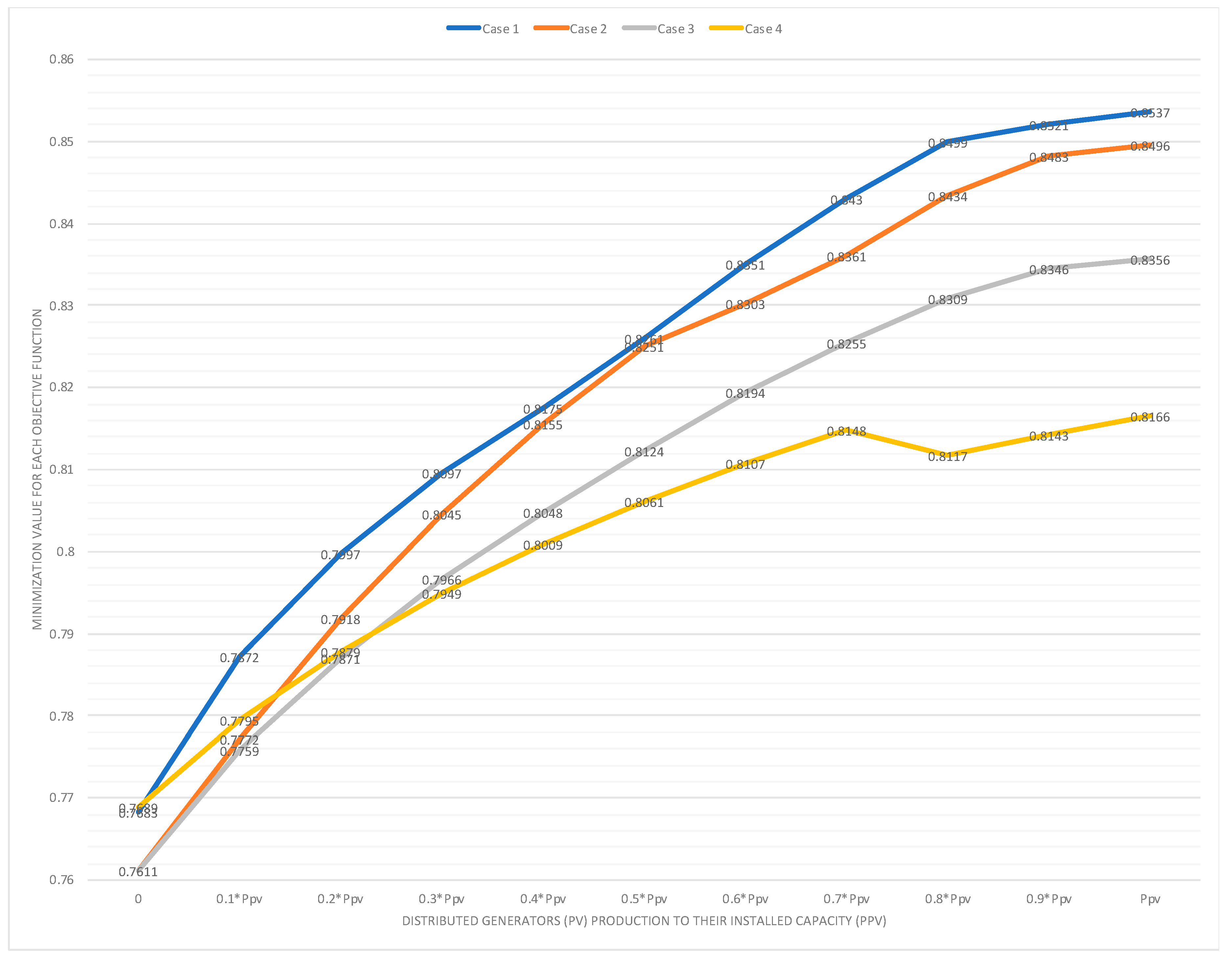
full DG prod	0.8537	0.8496	0.8356	0.8166

and Figure 3 show the calculated values for the objective function for each case; the values are increasing when the production from the renewables also increasing, since more load is able to be fed to the low voltage network distribution transformers without decreasing voltage at all points. The production is able to feed nearby loads; hence, the total load served is increasing without severely affecting voltage drop. The higher increase is observed when voltage drop has higher weighting factor for the case 1 and lower for case 4. The graphical representation of this interrelation shall normally provide perfect curves; however, due to the probabilistic approach applied, there could be minor rounding errors that do not substantially affect the results. The source code for this publication has been written on Matpower 6.0 [36,37] and Mathworks Matlab 2017a [38]. The Monte Carlo simulation was run on Aris high performance computing [39].

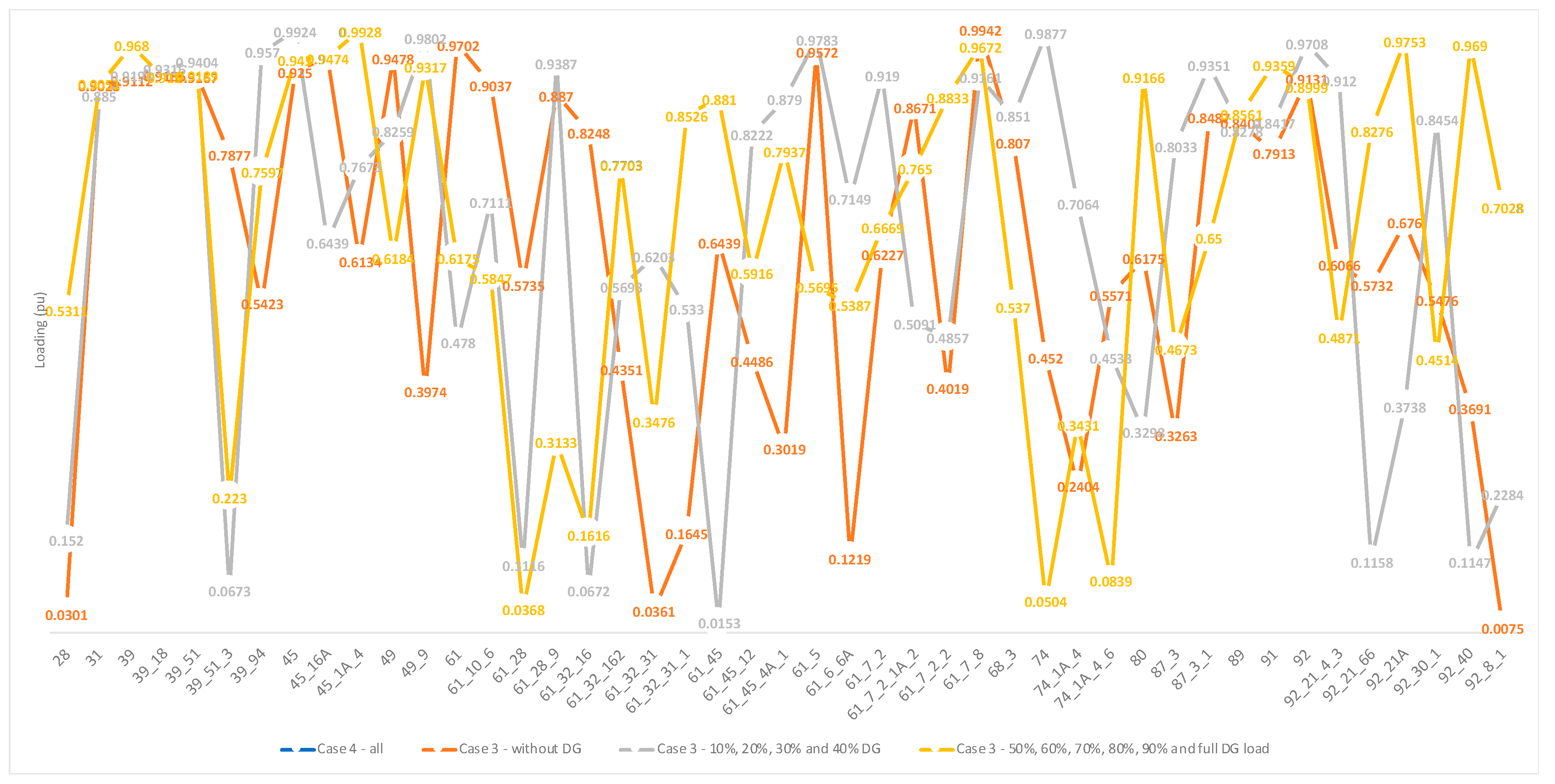
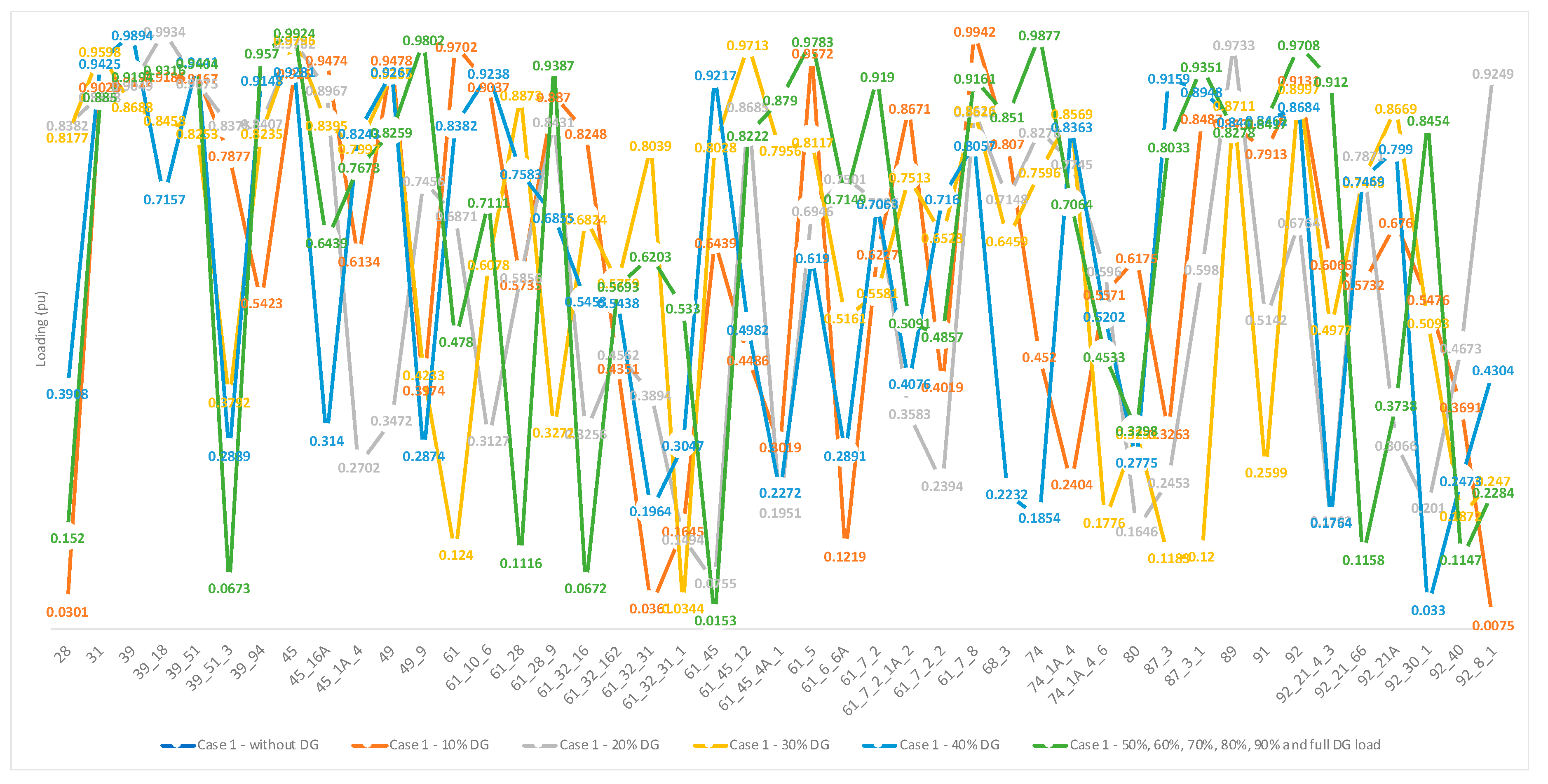
Table 6. Loading per node for case 1.

Node	0% DG	10% DG	20% DG	30% DG	40% DG	50–100% DG
1	83.8%	3.0%	83.8%	81.8%	39.1%	15.2%
2	88.6%	90.2%	88.6%	96.0%	94.3%	88.5%
4	90.5%	91.1%	90.5%	86.9%	98.9%	91.9%
6	97.6%	92.5%	97.6%	98.0%	92.8%	99.2%
7	34.7%	94.8%	34.7%	92.4%	92.7%	82.6%
10	68.7%	97.0%	68.7%	12.4%	83.8%	47.8%
14	82.8%	45.2%	82.8%	76.0%	18.5%	98.8%
15	16.5%	61.8%	16.5%	32.5%	27.8%	33.0%
19	97.3%	84.0%	97.3%	87.1%	84.4%	82.8%
20	51.4%	79.1%	51.4%	26.0%	84.6%	84.2%
22	67.6%	91.3%	67.6%	90.0%	86.8%	97.1%
25	99.3%	91.9%	99.3%	84.6%	71.6%	93.2%
26	90.8%	91.7%	90.8%	82.5%	94.4%	94.0%
28	83.8%	78.8%	83.8%	37.9%	28.9%	6.7%
27	84.1%	54.2%	84.1%	82.4%	91.5%	95.7%
29	89.7%	94.7%	89.7%	84.0%	31.4%	64.4%
31	27.0%	61.3%	27.0%	80.0%	82.4%	76.7%
9	74.6%	39.7%	74.6%	42.3%	28.7%	98.0%
34	31.3%	90.4%	31.3%	60.8%	92.4%	71.1%
40	58.6%	57.4%	58.6%	88.7%	75.8%	11.2%
41	84.3%	88.7%	84.3%	32.7%	68.6%	93.9%
45	32.6%	82.5%	32.6%	68.2%	54.5%	6.7%
50	45.6%	43.5%	45.6%	57.6%	54.4%	56.9%
46	38.9%	3.6%	38.9%	80.4%	19.6%	62.0%
49	14.9%	16.5%	14.9%	3.4%	30.5%	53.3%
53	7.6%	64.4%	7.6%	80.3%	92.2%	1.5%
59	86.9%	44.9%	86.9%	97.1%	49.8%	82.2%
60	19.5%	30.2%	19.5%	79.6%	22.7%	87.9%
61	69.5%	95.7%	69.5%	81.2%	61.9%	97.8%
64	75.0%	12.2%	75.0%	51.6%	28.9%	71.5%
66	70.9%	62.3%	70.9%	55.8%	70.6%	91.9%
117	35.8%	86.7%	35.8%	75.1%	40.8%	50.9%
69	23.9%	40.2%	23.9%	65.2%	71.6%	48.6%
67	86.1%	99.4%	86.1%	86.3%	80.6%	91.6%
12	71.5%	80.7%	71.5%	64.6%	22.3%	85.1%
16	77.5%	24.0%	77.5%	85.7%	83.6%	70.6%
71	59.6%	55.7%	59.6%	17.8%	52.0%	45.3%
18	24.5%	32.6%	24.5%	11.8%	91.6%	80.3%
75	59.8%	84.9%	59.8%	12.0%	89.5%	93.5%
96	17.9%	60.7%	17.9%	49.8%	17.6%	91.2%
94	78.7%	57.3%	78.7%	74.5%	74.7%	11.6%
92	30.7%	67.6%	30.7%	86.7%	79.9%	37.4%
98	20.1%	54.8%	20.1%	50.9%	3.3%	84.5%
99	46.7%	36.9%	46.7%	18.7%	24.7%	11.5%
101	92.5%	0.8%	92.5%	24.7%	43.0%	22.8%

,

Table 7. Loading per node for case 2.

Node	0% DG	10% DG	20–100% DG	Node	0% DG	10% DG	20–100% DG
1	3.0%	3.0%	15.2%	46	3.6%	3.6%	62.0%
2	90.2%	90.2%	88.5%	49	16.5%	16.5%	53.3%
4	91.1%	91.1%	91.9%	53	64.4%	64.4%	1.5%
6	92.5%	92.5%	99.2%	59	44.9%	44.9%	82.2%
7	94.8%	94.8%	82.6%	60	30.2%	30.2%	87.9%
10	97.0%	97.0%	47.8%	61	95.7%	95.7%	97.8%
14	45.2%	45.2%	98.8%	64	12.2%	12.2%	71.5%
15	61.8%	61.8%	33.0%	66	62.3%	62.3%	91.9%
19	84.0%	84.0%	82.8%	117	86.7%	86.7%	50.9%
20	79.1%	79.1%	84.2%	69	40.2%	40.2%	48.6%
22	91.3%	91.3%	97.1%	67	99.4%	99.4%	91.6%
25	91.9%	91.9%	93.2%	12	80.7%	80.7%	85.1%
26	91.7%	91.7%	94.0%	16	24.0%	24.0%	70.6%
28	78.8%	78.8%	6.7%	71	55.7%	55.7%	45.3%
27	54.2%	54.2%	95.7%	18	32.6%	32.6%	80.3%
29	94.7%	94.7%	64.4%	75	84.9%	84.9%	93.5%
31	61.3%	61.3%	76.7%	96	60.7%	60.7%	91.2%
9	39.7%	39.7%	98.0%	94	57.3%	57.3%	11.6%
34	90.4%	90.4%	71.1%	92	67.6%	67.6%	37.4%
40	57.4%	57.4%	11.2%	98	54.8%	54.8%	84.5%
41	88.7%	88.7%	93.9%	99	36.9%	36.9%	11.5%
45	82.5%	82.5%	6.7%	101	0.8%	0.8%	22.8%
50	43.5%	43.5%	56.9%

,

Table 8. Loading per node for case 3.

Node	0% DG	10% DG	20% DG	30% DG	40% DG	50–100% DG
1	3.0%	15.2%	15.2%	15.2%	15.2%	53.1%
2	90.2%	88.5%	88.5%	88.5%	88.5%	90.5%
4	91.1%	91.9%	91.9%	91.9%	91.9%	96.8%
6	92.5%	99.2%	99.2%	99.2%	99.2%	94.5%
7	94.8%	82.6%	82.6%	82.6%	82.6%	61.8%
10	97.0%	47.8%	47.8%	47.8%	47.8%	61.8%
14	45.2%	98.8%	98.8%	98.8%	98.8%	5.0%
15	61.8%	33.0%	33.0%	33.0%	33.0%	91.7%
19	84.0%	82.8%	82.8%	82.8%	82.8%	85.6%
20	79.1%	84.2%	84.2%	84.2%	84.2%	93.6%
22	91.3%	97.1%	97.1%	97.1%	97.1%	90.0%
25	91.9%	93.2%	93.2%	93.2%	93.2%	91.5%
26	91.7%	94.0%	94.0%	94.0%	94.0%	91.9%
28	78.8%	6.7%	6.7%	6.7%	6.7%	22.3%
27	54.2%	95.7%	95.7%	95.7%	95.7%	76.0%
29	94.7%	64.4%	64.4%	64.4%	64.4%	94.7%
31	61.3%	76.7%	76.7%	76.7%	76.7%	99.3%
9	39.7%	98.0%	98.0%	98.0%	98.0%	93.2%
34	90.4%	71.1%	71.1%	71.1%	71.1%	58.5%
40	57.4%	11.2%	11.2%	11.2%	11.2%	3.7%
41	88.7%	93.9%	93.9%	93.9%	93.9%	31.3%
45	82.5%	6.7%	6.7%	6.7%	6.7%	16.2%
50	43.5%	56.9%	56.9%	56.9%	56.9%	77.0%
46	3.6%	62.0%	62.0%	62.0%	62.0%	34.8%
49	16.5%	53.3%	53.3%	53.3%	53.3%	85.3%
53	64.4%	1.5%	1.5%	1.5%	1.5%	88.1%
59	44.9%	82.2%	82.2%	82.2%	82.2%	59.2%
60	30.2%	87.9%	87.9%	87.9%	87.9%	79.4%
61	95.7%	97.8%	97.8%	97.8%	97.8%	57.0%
64	12.2%	71.5%	71.5%	71.5%	71.5%	53.9%
66	62.3%	91.9%	91.9%	91.9%	91.9%	66.7%
117	86.7%	50.9%	50.9%	50.9%	50.9%	76.5%
69	40.2%	48.6%	48.6%	48.6%	48.6%	88.3%
67	99.4%	91.6%	91.6%	91.6%	91.6%	96.7%
12	80.7%	85.1%	85.1%	85.1%	85.1%	53.7%
16	24.0%	70.6%	70.6%	70.6%	70.6%	34.3%
71	55.7%	45.3%	45.3%	45.3%	45.3%	8.4%
18	32.6%	80.3%	80.3%	80.3%	80.3%	46.7%
75	84.9%	93.5%	93.5%	93.5%	93.5%	65.0%
96	60.7%	91.2%	91.2%	91.2%	91.2%	48.7%
94	57.3%	11.6%	11.6%	11.6%	11.6%	82.8%
92	67.6%	37.4%	37.4%	37.4%	37.4%	97.5%
98	54.8%	84.5%	84.5%	84.5%	84.5%	45.1%
99	36.9%	11.5%	11.5%	11.5%	11.5%	96.9%
101	0.8%	22.8%	22.8%	22.8%	22.8%	70.3%

and

Table 9. Loading per node for case 4.

Node	All Cases	Node	All Cases	Node	All Cases	Node	All Cases
1	53.1%	26	91.9%	49	85.3%	71	8.4%
2	90.5%	28	22.3%	53	88.1%	18	46.7%
4	96.8%	27	76.0%	59	59.2%	75	65.0%
6	94.5%	29	94.7%	60	79.4%	96	48.7%
7	61.8%	31	99.3%	61	57.0%	94	82.8%
10	61.8%	9	93.2%	64	53.9%	92	97.5%
14	5.0%	34	58.5%	66	66.7%	98	45.1%
15	91.7%	40	3.7%	117	76.5%	99	96.9%
19	85.6%	41	31.3%	69	88.3%	101	70.3%
20	93.6%	45	16.2%	67	96.7%
22	90.0%	50	77.0%	12	53.7%
25	91.5%	46	34.8%	16	34.3%

and their graphical representations Figure 4, Figure 5 and Figure 6 present the recommended loading per node for each examined case, according to the outcomes of the developed calculation procedures. For the case 1 (Table 6 and Figure 4), the obtained results indicate that most of the transformers can be fed near their installed capacity. However, there are connection points that when energy production from renewables is high, they need to keep their load low and vice versa. Other transformers, such as 49 and 15, need to be downscaled if these operational patterns are to be applied. In all cases, its proposed loading does not exceed 60% of their installed capacity. Another solution could be to further reinforce the line at these points.

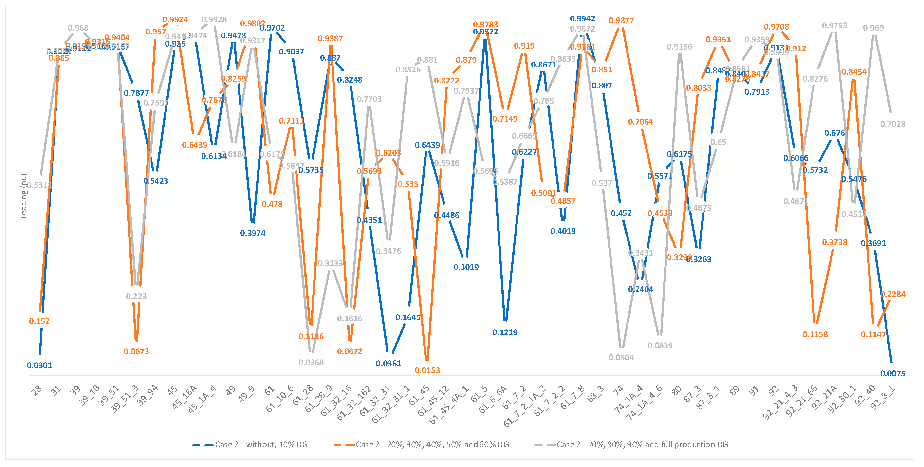
Considering case 2 (Table 7 and Figure 5), similar results are being observed. The proposed load for several transformers (15, 40, 49, 50, 69, 75, 92, 94, 99, 101) does not exceed 70% of their installed power at any production from the renewable energy sources. Similarly, the proposed load of the transformers 1, 40, 46 and 71 for case 3 (Table 8 and Figure 6) and 1, 7, 10, 12, 14, 16, 59, 61, 64, 66 and 98 for case 4 (Table 9 and Figure 4) does not exceed their installed power capacity. Note that these nodes are the points that are expected to receive more attention for downscaling and/or line reinforcing. Added to the above, it is necessary to highlight the impact of the considered distribution generation (DG) on the obtained results. In cases 1 and 3, the loading per node for DG from 50% to 100% of the installed capacity does not change. In case 2, DG from 20% to 100% provides the same results, since for case 4, the distribution generation does not affect the proposed loading of each transformer.

The proposed method is able to evaluate the performance of the line after reinforcement, even if this is done using meshed networks configuration. It can be used additionally to any other distribution optimization method. The results are able to propose specific operational points of the line based on the production of the connected distributed generations. In this case, the optimal loading of the line at each of its points is predefined. Given that according to the current operational procedures for the distribution lines it is not possible to control loading with such an accuracy, the applicability of the method is restrained.

The connection of new elements such as electric vehicles and storage, on one hand substantially enhances the capability of demand management and on the other hand there are limitations for lines’ expansion. Existing bibliography on the field supports this approach and provides solutions on this direction. Electric vehicles can be aggregated to a virtual power plant, being able to offer ancillary services [40]. This technology can be applied here to always have the operation near the optimal points [41]. However, it has to be mentioned that this procedure would potentially affect customers comfort due to the prioritization of network capacity over user immediate requirements for charging but with substantial benefit to grid flexibility and performance [42].

4. Conclusions

This paper proposes an innovative probabilistic method for evaluating the potential performance of meshed and radial distribution lines, improving electric energy distribution grids reinforcement decisions. It is developed as additional to the existing distribution networks optimization methods, offering a tool for performance evaluation. Furthermore, it serves to the creation of operational points to be used for demand management, if electric vehicle charging is completely controlled. This method is a useful tool for network planners, operators and large users, since they are more able to estimate the robustness of a given network after reinforcement and its capability to host electric vehicle loads. The operational points are loading patterns for the transformers of the low voltage distribution network that minimize voltage drop and maximize total loading. They are calculated for increasing production of the connected to the line distributed generators. Other distribution network lines are expected to have similar behavior. They shall present specific operational patterns and their reinforcement could be also evaluated using this method. Future work includes the investigation of the adoption of the appropriate protection schemes that will ensure the reliable and uninterruptable operation of the network.